Quantum Scattering by Multiple Slits—A Lippmann–Schwinger Approach

Abstract

We investigate the non-relativistic scattering of a plane wave by a vertical segment formulating the problem in terms of the Lippmann–Schwinger equation in two spatial dimensions. Adjusting the coupling strength function we show how to implement the scattering by a system of multiple slits and by a Cantor set. We present detailed calculations of the scattered wave function for the line segment, as well as for the single, double, and multiple slits. We define reflection and transmission functions that are position-dependent in a defined region. From these results, we obtain the probability densities and differential and total cross-sections for these problems.

1. Introduction

Studies concerning non-relativistic quantum effects in spatial, plane or even one-dimensional systems often focus on the scattering phenomena, in which the scatterer is always represented as a potential [1,2]. The analysis is constructed based on the knowledge of the scattering amplitudes and cross-sections, usually formulated using Schrödinger or Lippmann–Schwinger (LS) equation [3], and the motivations vary from pure theoretical interest, such as applications of special functions in billiards problems [4,5,6] and spatial barriers [7], a challenging equation [8], or an unexplored gap in the literature [9], to the possible construction of nanostructured or low-dimensional systems which could exhibit novel or unexpected properties, like curved quantum wires [10,11,12,13,14,15,16] or quantum corrals [17].

Another interesting line of research follows the path of the analog gravity program. In this context, acoustic scattering in fluids like Bose–Einstein condensates is related to the scattering of a scalar field in the event horizon of a black hole. Recent investigations also suggested that quantum particles coupled to curved surfaces can be used within this program [18]. Interestingly, what started as a way to probe into black hole mechanics can now be used to inquire into new and rich physics in quantum field theory and condensed matter physics [19], which is also the goal of quantum scattering theory.

The scope of applications is quite rich. However, the kernel of scattering remains the same, made of refraction, diffraction, interference, and the key mental picture for explaining scattering phenomena continues to be the double-slit experiment [20]. However, the scattering of a plane wave by a double slit has found no exact, closed-form solution within the confines of quantum theory. The current study is concerned with simplifying this problem: scattering a plane wave by a straight line segment. It is a challenging mathematical problem because the parametric description of the scatterer either requires the usage of Green’s function in Cartesian coordinates (possible but undesirable) or breaks the symmetry of any coordinate system but the rectangular one. This problem is certainly in need of a solution, and in response, we choose to use the second approach, the non-rectangular coordinate system. An exact solution can be achieved by employing a method formulated in Ref. [8] to solve the LS equation for this problem. One can write the potential representing the scatterer in terms of delta functions, a technique introduced in Refs. [21,22], which is known as the boundary-wall method. The delta functions have been used [23] to reproduce various known [24,25] physical effects—such as, for instance, the Casimir effect—and may be the most straightforward mathematical basis to use in expanding a physical potential that still gives meaningful results. Such boundary-wall potentials have been experimentally realized via optical methods [26] with high success. Several applications of the boundary-wall method, in particular, have been made in the field of photonic crystals [27] and quantum billiards [28] as well as scattering involving obstacles [29].

The outline for the paper is as follows. In Section 2, we formulate the non-relativistic scattering problem of a plane wave by a finite segment in terms of the LS integral equation. After analytical manipulation, we obtain a system of integral equations that can be transformed into a first-order ordinary differential equations system. We solve this system numerically to obtain the solution of the LS equation for the scattering of a plane wave impinging upon a potential built as a Dirac delta distribution running along a finite segment. Then, we present density plots for the solution for various interesting values of the wave number k as well as the differential and total cross-sections. In Section 3, we make use of the knowledge and results obtained from the previous section to model the single slit, presenting the numerical solution through density plots. Also, these results allow us to investigate the differential and total cross-sections. We carry out similar processes in Section 4 and Section 5 for the double-slit and multiple-slit potentials modeled by a Cantor set, respectively. We present our final remarks and the perspectives for future investigations in Section 6.

2. Scattering by a Finite Segment

Let us model the barriers using the so-called boundary-wall potentials. As one learns from distribution theory [30], the correct way to attach a given distribution—singular or regular alike—in a hypersurface is introducing such distribution as an integral with position-dependent weight (or coupling strength) $\gamma \left(\mathbf{r}\right)$; this function determines the intensity or the strength of the interactions with the potential. Thus, let us consider the potential

$$V(r^{\prime },{\theta }^{\prime })={\int }_C\gamma \left(s\right){\displaystyle \frac{\delta ({\theta }^{\prime }-s^{\prime })\delta (r^{\prime }-x_{0}sec{s}^{\prime })}{J}} dl,$$

(1)

where the line element for the curve $r=x_{0}secs$ with $x_0$ representing the distance from the origin in the x-coordinate is written as $dl=x_0{sec}^{2}sds$, with s changing from $-{\theta }_0$ to ${\theta }_0$, where ${\theta }_0$ defines the length L of the line segment via $cos{\theta }_0=x_0/R$ with the radius R as $L=2Rsin{\theta }_0=2\sqrt{R^2-x_0^2}$, $\delta (·)$ is the Dirac delta function and J is the Jacobian.

In the position representation $\left\{\right|\mathbf{r}⟩\}$, after integrating over $r^{\prime }$ and ${\theta }^{\prime }$, the LS equation reads

$$\psi (r,\theta )=\phi (r,\theta )+A{\int }_C\gamma \left(s\right)G_0^{+}\left(r,\theta |s,{\theta }_0\right)\psi (s,{\theta }_0) ds,$$

(2)

where $\mathbf{r}=(r,\theta )$ and ${\mathbf{r}}^{\prime }=(r^{\prime },{\theta }^{\prime })$ represent a point in space and a point at the source, respectively. Since the potential (1) is composed of Dirac delta functions, the boundary conditions—which are encompassed by the Green’s function—imposed by such distributions are the continuity of the wave function crossing the barrier, and a jump discontinuity in the first derivative also crossing the barrier. Moreover, the radial solution must be regular at the origin and finite when $r\to \infty$. The constant $A=2m^{*}/{\hslash }^2$, where $m^{*}$ is the particle mass and ℏ is the reduced Planck constant. $G_0^{+}\left(\mathbf{r}\right|{\mathbf{r}}^{\prime })$ is the two-dimensional free Green’s function (where the “+” sign indicates the retarded Green’s function, where integration is being done over the positive integration path), whose closed form is given by [31,32,33].

$$G_0^{+}\left(\mathbf{r}\right|{\mathbf{r}}^{\prime })=-{\displaystyle \frac{i}{4}}{H}_0^{\left(1\right)}\left(k|\mathbf{r}-{\mathbf{r}}^{\prime }|\right),$$

(3)

where $H_0^{\left(1\right)}$ is the first kind of Hankel function of order zero. We also define $R=|\mathbf{r}-{\mathbf{r}}^{\prime }|$ and k is the particle wave number.

Using the known bilinear expansion [34], one writes the free Green’s function,

$$G_0^{+}\left(\mathbf{r}\right|{\mathbf{r}}^{\prime })=-{\displaystyle \frac{i}{4}}\sum _{l=-\infty }^{\infty }{J}_l\left(k{r}_{<}\right)H_l^{\left(1\right)}\left(k{r}_{>}\right)exp\left[il(\theta -{\theta }^{\prime })\right],$$

(4)

in terms of the ordinary Bessel and first-kind Hankel functions—$J_l$ and $H_l^{\left(1\right)}$—respectively. Substituting Green’s function (4) into the LS Equation (2) yields

$$\begin{array}{c}\psi (r,\theta )=\phi (r,\theta )-{\displaystyle \frac{iA}{4}}\sum _{l=-\infty }^{\infty }{e}^{il\theta }\\ \hspace{1em}\hspace{1em}\hspace{1em}\hspace{1em}\hspace{1em}\hspace{1em}\hspace{1em}\hspace{1em}\times {\int }_{-{\theta }_0}^{{\theta }_0}{x}_0{sec}^2\left(s\right)\gamma \left(s\right)J_l\left(k{r}_{<}\right)H_l^{\left(1\right)}\left(k{r}_{>}\right)e^{-ils}\psi (x_{0}sec\left(s\right),s) ds,\end{array}$$

(5)

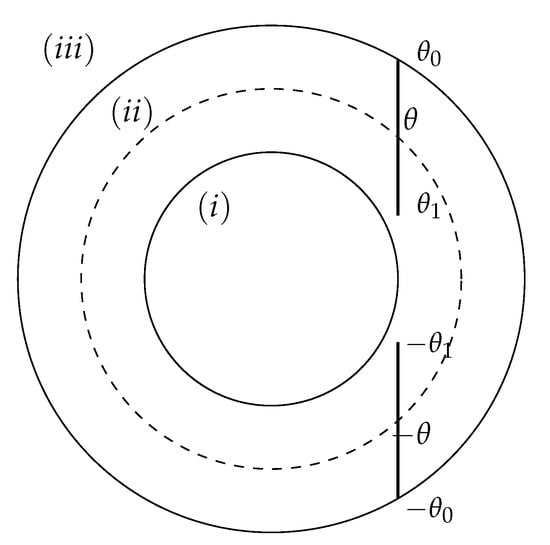
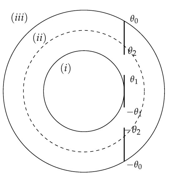
where we use the standard notation $r_{<}=min(r,x_{0}sec\left(\theta \right))$ and $r_{>}=max(r,x_{0}sec\left(\theta \right))$. The LS Equation (5) naturally defines three regions in the plane as illustrated in Figure 1.

2.1. Solution for Exterior Region $r>R$

In this region (the exterior of the larger circumference in Figure 1), there is no integration, thus, one can straightforwardly write:

$$\begin{array}{c}\psi (r,\theta )=\phi (r,\theta )-{\displaystyle \frac{iA}{4}}\sum _{l=-\infty }^{\infty }{e}^{il\theta }{H}_l^{\left(1\right)}\left(kr\right)\hfill \\ \hfill \hspace{1em}\hspace{1em}\hspace{1em}\hspace{1em}\hspace{1em}\hspace{1em}\hspace{1em}\hspace{1em}\hspace{1em} \times {\int }_{-{\theta }_0}^{{\theta }_0}{x}_0{sec}^2\left(s\right)\gamma \left(s\right)J_l(k{x}_{0}sec\left(s\right))e^{-ils}\psi (x_{0}sec\left(s\right),s) ds,\end{array}$$

(6)

Introducing the quantities

$${\beta }_l={\int }_{-{\theta }_0}^{{\theta }_0}{x}_0{sec}^2\left(s\right)\gamma \left(s\right)J_l(k{x}_{0}sec\left(s\right))e^{-ils}\psi (x_{0}sec\left(s\right),s) ds,$$

(7)

and if one is able to calculate those, the LS solution for $r>R$ reads

$${\psi }_1(r,\theta )=\phi (r,\theta )-{\displaystyle \frac{iA}{4}}\sum _{l=-\infty }^{\infty }{\beta }_l\left({\theta }_0\right)H_l^{\left(1\right)}\left(kr\right)e^{il\theta }.$$

(8)

In order to calculate the coefficients (7), we multiply Equation (8) by the factor $x_0{sec}^2\left(\theta \right)J_{l^{\prime }}(k{x}_{0}sec\left(\theta \right))e^{-i{l}^{\prime }\theta }\gamma \left(\theta \right)$ with $l^{\prime }$ being an integer, evaluate at $r=x_{0}sec\left(\theta \right)$ and integrate it over the angular coordinate from $-{\theta }_0$ to ${\theta }_0$. Then, a system of linear equations is obtained:

$${\beta }_{l^{\prime }}\left({\theta }_0\right)=c_{l^{\prime }}\left({\theta }_0\right)-{\displaystyle \frac{iA}{4}}\sum _{l=-\infty }^{\infty }{\beta }_{l^{\prime }}\left({\theta }_0\right){\left(JH\right)}_{l^{\prime }l},$$

(9)

where we define

$$c_{l^{\prime }}\left({\theta }_0\right)={\int }_{-{\theta }_0}^{{\theta }_0}{x}_0{sec}^2\left(\theta \right)J_{l^{\prime }}(k{x}_{0}sec\left(\theta \right))e^{-i{l}^{\prime }\theta }\gamma \left(\theta \right)\chi (x_{0}sec\left(\theta \right),\theta ) d\theta ,$$

(10)

$${\left(JH\right)}_{l^{\prime }l}={\int }_{-{\theta }_0}^{{\theta }_0}{x}_0{sec}^2\left(\theta \right)J_{l^{\prime }}(k{x}_{0}sec\left(\theta \right))e^{i(l-l^{\prime })\theta }\gamma \left(\theta \right)H_l^{\left(1\right)}(k{x}_{0}sec\left(\theta \right)) d\theta .$$

(11)

Considering the incident wave to be monochromatic, i.e.,

$$\phi (r,\theta )=\sum _{l=-\infty }^{\infty }{i}^l{e}^{il(\theta -\varphi )}{J}_l\left(kr\right),$$

(12)

where $\varphi$ is the incidence angle, one obtains

$$c_{l^{\prime }}\left({\theta }_0\right)=\sum _{l=-\infty }^{\infty }{i}^l{e}^{-il\varphi }{\left(JJ\right)}_{l^{\prime }l} ,$$

(13)

where

$${\left(JJ\right)}_{l^{\prime }l}={\int }_{-{\theta }_0}^{{\theta }_0}{x}_0{sec}^2\left(\theta \right)J_{l^{\prime }}(k{x}_{0}sec\left(\theta \right))J_l(k{x}_{0}sec\left(\theta \right))e^{i(l-l^{\prime })\theta }\gamma \left(\theta \right) d\theta .$$

(14)

Solving the system (9), one obtains the coefficients ${\omega }_l$ and, substituting those into Equation (8), one obtains the solution for the LS Equation (5) in the exterior region.

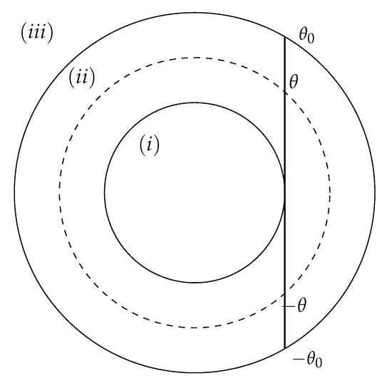
Figure 1. Secant segment cutting x-axis at $x=x_0$, starting at $\theta =-{\theta }_0$ and ending at $\theta ={\theta }_0$, with the length $L=2Rsin{\theta }_0$. The three regions are defined: (i) interior region where $0\le r\le x_0$ (inside middle circumference), (ii) annular region where $x_0\le r\le R$, and (iii) exterior region where $r>R$ (outside larger circumference). See text for details.

2.2. Solution for Ring Region $x_0\le r\le R$

In this region, there are both the contributions ($r_{<}=r$, $r_{>}=x_{0}sec\left(\theta \right)$) and ($r_{<}=x_{0}sec\left(\theta \right)$, $r_{>}=r$), that is, the integral over the barrier to be split into two integrals:

$$\begin{array}{c}\psi (r,\theta )=\phi (r,\theta )-{\displaystyle \frac{iA}{4}}\sum _{l=-\infty }^{\infty }{e}^{il\theta }\hfill \\ \hspace{1em}\times \left\{{\int }_{-{\theta }_0}^{-\theta }+{\int }_{\theta }^{{\theta }_0}\right\}ds (x_0{sec}^2\left(s\right)\gamma \left(s\right)H_l^{\left(1\right)}(k{x}_{0}sec\left(s\right))e^{-ils}\psi (x_{0}sec\left(s\right),s)J_l\left(kr\right)\\ \hfill +{\int }_{-\theta }^{-\theta }ds x_0{sec}^2\left(s\right)\gamma \left(s\right)J_l(k{x}_{0}sec\left(s\right))e^{-ils}\psi (x_{0}sec\left(s\right),s)H_l^{\left(1\right)}\left(kr\right)).\end{array}$$

(15)

Then, we define two functions which depend on the angular momentum quantum number l, and since $\theta =arccos(x_0/r)$, the integral (15) depends also on the position r:

$$R_l\left(r\right)=\left\{{\int }_{-{\theta }_0}^{-\theta }+{\int }_{\theta }^{{\theta }_0}\right\}ds x_0{sec}^2\left(s\right)\gamma \left(s\right)H_l^{\left(1\right)}(k{x}_{0}sec\left(s\right))e^{-ils}\psi (x_{0}sec\left(s\right),s)$$

(16)

and

$$T_l\left(r\right)={\int }_{-\theta }^{-\theta }ds x_0{sec}^2\left(s\right)\gamma \left(s\right)J_l(k{x}_{0}sec\left(s\right))e^{-ils}\psi (x_{0}sec\left(s\right),s),$$

(17)

so the LS solution in this region to be written as

$${\psi }_2(r,\theta )=\phi (r,\theta )-{\displaystyle \frac{iA}{4}}\sum _{l=-\infty }^{\infty }{e}^{il\theta }\left[R_l\left(r\right)J_l\left(kr\right)+T_l\left(r\right)H_l^{\left(1\right)}\left(kr\right)\right].$$

(18)

One needs to determine the two sets of functions $T_l$ (16) and $R_l$ (17). Inside the annular region $x_0\le r\le R$, the functions $T_l$ and $R_l$ can be interpreted as position-dependent transmission and reflection functions, respectively, since Hankel functions represent propagating waves (to infinity) and ordinary Bessel functions represent stationary waves. Thus, at the extremes of this region, $T_l\left(r\right)$ and $R_l\left(r\right)$ are reduced to the known, constant, transmission and reflection amplitudes. Let us first multiply Equation (15) by $x_0{sec}^2\left(\theta \right)\gamma \left(\theta \right)H_{l^{\prime }}^{\left(1\right)}(k{x}_{0}sec\left(s\right))e^{i{l}^{\prime }\theta }$, evaluate at $r=sec\left({\theta }_0\right)$ and integrate, then receiving Equation (19) below. The second step is to multiply Equation (15) by $x_0{sec}^2\left(\theta \right)\gamma \left(\theta \right)J_{l^{\prime }}(k{x}_{0}sec\left(s\right))e^{i{l}^{\prime }\theta }$, evaluate at $r=sec\left({\theta }_0\right)$ and integrate from $r^{\prime }$ to L then receiving Equation (20) below. Instead of finding a system of linear equations, one obtains a system of Volterra integral equations [35], namely

$$\begin{array}{ccc}\hfill R_{l^{\prime }}\left(r\right)& =& \left\{{\int }_{-{\theta }_0}^{-\theta }+{\int }_{\theta }^{{\theta }_0}\right\}d\theta x_0{sec}^2\left(\theta \right)\gamma \left(\theta \right)H_{l^{\prime }}^{\left(1\right)}(k{x}_{0}sec\left(\theta \right))e^{-i{l}^{\prime }s}\phi (x_{0}sec\left(\theta \right),\theta )\hfill \\ & -& {\displaystyle \frac{iA}{4}}\left\{{\int }_{-{\theta }_0}^{-\theta }+{\int }_{\theta }^{{\theta }_0}\right\}d\theta x_0{sec}^2\left(\theta \right)\gamma \left(\theta \right)H_{l^{\prime }}^{\left(1\right)}(k{x}_{0}sec\left(\theta \right))e^{-i{l}^{\prime }\theta }\sum _{l=-\infty }^{\infty }{e}^{il\theta }\hfill \\ & \times & \left[R_l(x_{0}sec\left(\theta \right))J_l(k{x}_{0}sec\left(\theta \right))+T_l(x_{0}sec\left(\theta \right))H_l^{\left(1\right)}(k{x}_{0}sec\left(\theta \right))\right],\hfill \end{array}$$

(19)

and

$$\begin{array}{ccc}\hfill T_{l^{\prime }}\left(r\right)& =& {\int }_{-\theta }^{\theta }d\theta x_0{sec}^2\left(\theta \right)\gamma \left(\theta \right)J_{l^{\prime }}(k{x}_{0}sec\left(\theta \right))e^{-i{l}^{\prime }s}\phi (x_{0}sec\left(\theta \right),\theta )\hfill \\ & -& {\displaystyle \frac{iA}{4}}{\int }_{-\theta }^{\theta }d\theta x_0{sec}^2\left(\theta \right)\gamma \left(\theta \right)J_{l^{\prime }}(k{x}_{0}sec\left(\theta \right))e^{-i{l}^{\prime }\theta }\sum _{l=-\infty }^{\infty }{e}^{il\theta }\hfill \\ & \times & \left[R_l(x_{0}sec\left(\theta \right))J_l(k{x}_{0}sec\left(\theta \right))+T_l(x_{0}sec\left(\theta \right))H_l^{\left(1\right)}(k{x}_{0}sec\left(\theta \right))\right].\hfill \end{array}$$

(20)

The approach to solve such a system is [36] to take the first derivative with respect to the integration limit $\theta$. Then the systems (19) and (20) transforms into a first-order ordinary differential equation (ODE) system:

$$\begin{array}{ccc}\hfill R_{l^{\prime }}^{\prime }\left(r\right)& =& -x_0{sec}^2\left(\theta \right){\displaystyle \frac{d\theta }{dr}}{H}_{l^{\prime }}^{\left(1\right)}(k{x}_{0}sec\left(\theta \right))\hfill \\ & \times & \left[\gamma (-\theta )e^{i{l}^{\prime }\theta }\phi (x_{0}sec\left(\theta \right),-\theta )+\gamma \left(\theta \right)e^{-i{l}^{\prime }\theta }\phi (x_{0}sec\left(\theta \right),\theta )\right]\hfill \\ & +& {\displaystyle \frac{iA}{4}}\sum _{l=-\infty }^{\infty }{x}_0{sec}^2\left(\theta \right)H_{l^{\prime }}^{\left(1\right)}(k{x}_{0}sec\left(\theta \right))\left[\gamma (-\theta )e^{-i(l-l^{\prime })\theta }+\gamma \left(\theta \right)e^{i(l-l^{\prime })\theta }\right]\hfill \\ & \times & \left[R_l(x_{0}sec\left(\theta \right))J_l(k{x}_{0}sec\left(\theta \right))+T_l(x_{0}sec\left(\theta \right))H_l^{\left(1\right)}(k{x}_{0}sec\left(\theta \right))\right]{\displaystyle \frac{d\theta }{dr}}\hfill \end{array}$$

(21)

and

$$\begin{array}{ccc}\hfill T_{l^{\prime }}^{\prime }\left(r\right)& =& x_0{sec}^2\left(\theta \right){\displaystyle \frac{d\theta }{dr}}{J}_{l^{\prime }}(k{x}_{0}sec\left(\theta \right))\hfill \\ & \times & \left[\gamma (-\theta )e^{i{l}^{\prime }\theta }\phi (x_{0}sec\left(\theta \right),-\theta )+\gamma \left(\theta \right)e^{-i{l}^{\prime }\theta }\phi (x_{0}sec\left(\theta \right),\theta )\right]\hfill \\ & -& {\displaystyle \frac{iA}{4}}\sum _{l=-\infty }^{\infty }{x}_0{sec}^2\left(\theta \right)J_{l^{\prime }}(k{x}_{0}sec\left(\theta \right))\left[\gamma (-\theta )e^{-i(l-l^{\prime })\theta }+\gamma \left(\theta \right)e^{i(l-l^{\prime })\theta }\right]\hfill \\ & \times & \left[R_l(x_{0}sec\left(\theta \right))J_l(k{x}_{0}sec\left(\theta \right))+T_l(x_{0}sec\left(\theta \right))H_l^{\left(1\right)}(k{x}_{0}sec\left(\theta \right))\right]{\displaystyle \frac{d\theta }{dr}}\hfill \end{array}$$

(22)

or, in the radial coordinate:

$$\begin{array}{ccc}\hfill R_{l^{\prime }}^{\prime }\left(r\right)& =& -{\displaystyle \frac{r{H}_{l^{\prime }}^{\left(1\right)}\left(kr\right)}{\sqrt{r^2-x_0^2}}}\left\{\left[\gamma \left(-arccos\left({\displaystyle \frac{x_0}{r}}\right)\right)e^{i{l}^{\prime }arccos\left({\displaystyle \frac{x_0}{r}}\right)}\chi \left(r,-arccos\left({\displaystyle \frac{x_0}{r}}\right)\right)\right.\right.\hfill \\ & +& \left.\gamma \left(arccos\left({\displaystyle \frac{x_0}{r}}\right)\right)e^{-i{l}^{\prime }arccos\left({\displaystyle \frac{x_0}{r}}\right)}\chi \left(r,arccos\left({\displaystyle \frac{x_0}{r}}\right)\right)\right]\hfill \\ & +& {\displaystyle \frac{i}{4}}\sum _{l=-\infty }^{\infty }\left[\gamma \left(-arccos\left({\displaystyle \frac{x_0}{r}}\right)\right)e^{-i(l-l^{\prime })arccos\left({\displaystyle \frac{x_0}{r}}\right)}+\gamma \left(arccos\left({\displaystyle \frac{x_0}{r}}\right)\right)e^{i(l-l^{\prime })arccos\left({\displaystyle \frac{x_0}{r}}\right)}\right]\hfill \\ & \times & \left.\left[R_l\left(r\right)J_l\left(kr\right)+T_l\left(r\right)H_l^{\left(1\right)}\left(kr\right)\right]\right\}\hfill \end{array}$$

(23)

and

$$\begin{array}{ccc}\hfill T_{l^{\prime }}^{\prime }\left(r\right)& =& -{\displaystyle \frac{r{J}_{l^{\prime }}\left(kr\right)}{\sqrt{r^2-x_0^2}}}\left\{\left[\gamma \left(-arccos\left({\displaystyle \frac{x_0}{r}}\right)\right)e^{-i{l}^{\prime }arccos\left({\displaystyle \frac{x_0}{r}}\right)}\chi \left(r,-arccos\left({\displaystyle \frac{x_0}{r}}\right)\right)\right.\right.\hfill \\ & +& \left.\gamma \left(-arccos\left({\displaystyle \frac{x_0}{r}}\right)\right)e^{-i{l}^{\prime }arccos\left({\displaystyle \frac{x_0}{r}}\right)}\chi \left(r,-arccos\left({\displaystyle \frac{x_0}{r}}\right)\right)\right]\hfill \\ & +& {\displaystyle \frac{iA}{4}}\sum _{l=-\infty }^{\infty }\left[\gamma \left(-arccos\left({\displaystyle \frac{x_0}{r}}\right)\right)e^{-i(l-l^{\prime })arccos\left({\displaystyle \frac{x_0}{r}}\right)}+\gamma \left(arccos\left({\displaystyle \frac{x_0}{r}}\right)\right)e^{i(l-l^{\prime })arccos\left({\displaystyle \frac{x_0}{r}}\right)}\right]\hfill \\ & \times & \left.\left[R_l\left(r\right)J_l\left(kr\right)+T_l\left(r\right)H_l^{\left(1\right)}\left(kr\right)\right]\right\}.\hfill \end{array}$$

(24)

Considering the definitions of $T_l\left(r\right)$ and $R_l\left(r\right)$ (16) and (17), we readily write the initial conditions: $T_l\left(x_0\right)=0$ and $R_l\left(R\right)=0$. In other words, one has a two-point boundary value problem formulated in terms of a coupled system of first-order ODEs.

2.3. Solution for Interior Region $0\le r\le x_0$

In this region (the smaller (inner) circumference in Figure 1), the integration variable s is always smaller then $x_{0}sec\left(\theta \right)$; then, in the LS Equation (5), one must have $r_{<}=r$ and $r_{>}=x_{0}sec\left(s\right)$, and

$$\psi (r,\theta )=\phi (r,\theta )-{\displaystyle \frac{iA}{4}}\sum _{l=-\infty }^{\infty }{J}_l\left(kr\right)e^{il\theta }{\int }_{-{\theta }_0}^{{\theta }_0}{x}_0{sec}^2\left(s\right)\gamma \left(s\right)H_l^{\left(1\right)}(k{x}_{0}sec\left(s\right))e^{-ils}\psi (x_{0}sec\left(s\right),s) ds,$$

(25)

so that introducing the definition

$${\alpha }_l={\int }_{-{\theta }_0}^{{\theta }_0}{x}_0{sec}^2\left(s\right)\gamma \left(s\right)H_l^{\left(1\right)}(k{x}_{0}sec\left(s\right))e^{-ils}\psi (x_{0}sec\left(s\right),s) ds,$$

(26)

and being able of calculating the coefficients ${\alpha }_l\left({\theta }_0\right)$ and inputting them into Equation (25), the solution of the LS equation in this region reads

$${\psi }_3(r,\theta )=\phi (r,\theta )-{\displaystyle \frac{iA}{4}}\sum _{l=-\infty }^{\infty }{\alpha }_l\left({\theta }_0\right)J_l\left(kr\right)e^{il\theta }.$$

(27)

Proceeding further the way it is done in Section 2.1 and Section 2.2, we multiply Equation (25) by $x_0{sec}^2\left(\theta \right)$$H_{l^{\prime }}^{\left(1\right)}(k{x}_{0}sec\left(\theta \right))e^{-i{l}^{\prime }\theta }\gamma \left(\theta \right)$, evaluate at $r=x_{0}sec\left(\theta \right)$ and integrate over $\theta$ from $-{\theta }_0$ to ${\theta }_0$. One concludes that the coefficients (26) must also satisfy a system of linear equations

$${\alpha }_{l^{\prime }}\left({\theta }_0\right)=d_{l^{\prime }}\left({\theta }_0\right)-{\displaystyle \frac{iA}{4}}\sum _{l=-\infty }^{\infty }{\alpha }_l\left({\theta }_0\right){\left(JH\right)}_{l{l}^{\prime }},$$

(28)

where $d_m$ is the integral of the incident plane wave (12) with $H_m^{\left(1\right)}\left(kr\right)\gamma \left(r\right)$, namely,

$$d_{l^{\prime }}\left({\theta }_0\right)=\sum _{l=-\infty }^{\infty }{i}^l{e}^{-il\varphi }{\left(JH\right)}_{l{l}^{\prime }},$$

(29)

where ${\left(JH\right)}_{lm}$ is given by Equation (10).

2.4. Complete Solution

Combining the results obtained above—Equations (8), (18), and (27)—one writes the sought solution of the LS Equation (5) as

$$\psi (r,\theta )=\left\{\begin{array}{cc}{\psi }_1(r,\theta )\hspace{1em}\hfill & \mathrm{for} r\ge R,\hfill \\ {\psi }_2(r,\theta )\hspace{1em}\hfill & \mathrm{for} x_0\le r\le R,\hfill \\ {\psi }_3(r,\theta )\hspace{1em}\hfill & \mathrm{for} r\le x_0,\hfill \end{array}\right.$$

(30)

the wave function is obtained for the scattering of a plane wave by a finite line segment valid on the whole plane. One can then solve the systems obtained numerically, using the Mathematica software, in order to calculate the coefficients and the position-dependent reflection and transmission functions. Convergence of the series at infinity is not problematic, since, for a fixed z, the asymptotic behaviour [37,38] of Bessel functions is $J_l\left(z\right)\to 0$ if $l>z$.

Figure 2 shows the two-dimensional projection of the three-dimensional probability density functions for the scattering of a palne wave by a single slit at different ks. One can notice in Figure 2 the wave function symmetry for the particle that arrives perpendicularly on the density plots. One can also observe the reflection due to the barrier on the left side of the images. Furthermore, at the end of the segment, the diffraction occurring with the wave surrounding the obstacle can be noticed. It can be also noted that, depending on the initial momentum k magnitude, there is a certain probability density just after the barrier, being observable for higher values of the momentum.

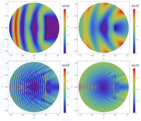
Figure 2. The probability density ${r|\Psi |}^2$ for the scattering of a plane wave by a finite segment which starts at a distance $x_0=1/2$ from the origin at the angle $\theta =\pi /4$ over to $\theta =-\pi /4$ for incident wave numbers $k=2\pi$ (upper), $12\pi$ (lower left) and $16\pi$ (lower right). The segment coupling constant used is set to $\gamma =100$ and the incident scattering angle to ${\theta }_0=0$. Black vertical segments represent the boundary walls.

Using the expression (8) for the exterior wave function, one can now make use of the asymptotic behavior of the Hankel function, that being

$$H_l^{\left(1\right)}\left(z\right)\to \sqrt{{\displaystyle \frac{2}{\pi z}}}exp\left[i\left(z-{\displaystyle \frac{l\pi }{2}}-{\displaystyle \frac{\pi }{4}}\right)\right],$$

(31)

which upon been substituted in Equation (8) yields the scattering amplitude

$$f\left(\theta \right)=-{\displaystyle \frac{iA}{4}}\sqrt{{\displaystyle \frac{2}{\pi k}}}{e}^{-i/4}\sum _{l=-\infty }^{\infty }{i}^{-l}{e}^{il\theta }{\beta }_l.$$

(32)

Figure 3 shows the differential cross-section for the scattering of a plane wave, as a function of the scattering angle $\theta$, over a finite segment for three different wave momenta. One can notice that in directions perpendicular to the direction of incidence, the plots present their lowest values. The maxima found at the angles zero and 2$\pi$ represent the wave that is transmitted by the barrier, while the peaks at $\pi$ represent the wave reflected by the barrier.

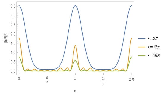
Figure 3. The differential cross-section $d\sigma /d\Omega$, where $\Omega$ is the solid angle, for the scattering of a plane wave, as a function of the scattering angle $\theta$, over a finite segment for three different wave momenta $k=2\pi ,12\pi \mathrm{and} 16\pi$, as indicated. The coupling constant used is set to $\gamma =100$ and the incident scattering angle to ${\theta }_0$ = 0.

Once one obtains the differential cross-section, one needs to integrate over the angles, acquiring thus the total cross-section ${\sigma }_T$, which we plot in Figure 4. Figure 4 (left) shows the total cross-section as a function of the incident wave number k. Note that the cross-section increases for a harder barrier (higher $\gamma$, green curve) exhibiting three sharp peaks. When $k>15$, all three curves tend to a similar behavior, that is, scattering does not happen for high k. Figure 4 (right) shows the total cross-section as a function of the coupling strength. For $k=4\pi$, the total cross-section is almost an even function, while for higher wave number, the cross-section increases for the attractive barrier, $\gamma <0$. For positive $\gamma$, both Figure 4 (left) and Figure 4 (right) demonstrate that no scattering happens as k increases.

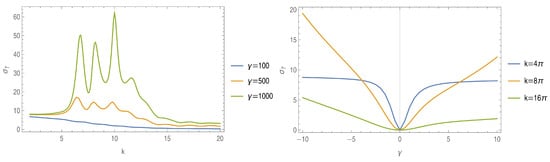
Figure 4. The total cross-section ${\sigma }_T$ for the scattering of a plane wave through a finite segment as a function of the momentum k and different coupling constants, as indicated (left), and of the coupling constant $\gamma$ and different wave numbers, as indicated (right). The incident scattering angle is set to ${\theta }_0=0$.

3. Single Slit

Given the results of Section 2 let us now solve the problem of a plane wave scattering by a single slit. In order to produce a plain slit barrier, let us consider the same boundary-wall potential (1), but now with a coupling function defined by parts as

$$\gamma \left(\theta \right)=\left\{\begin{array}{cc}1& \mathrm{for} -{\theta }_0\le \theta \le -{\theta }_1,\\ 0& \mathrm{for} -{\theta }_1\le \theta \le {\theta }_1,\\ 1& \mathrm{for} {\theta }_1\le \theta \le {\theta }_0,\end{array}\right.$$

(33)

where ${\theta }_1<{\theta }_0$. The LS Equation (5) then defines three regions as shown in Figure 5.

Figure 5. Secant segment at $x=x_0$, starting at $\theta =-{\theta }_0$ and ending at $\theta ={\theta }_0$, with coupling function defined by parts (33) in order to produce a single slit. Simiar to Figure 1, here, three regions are defined: (i) interior region where $0\le r\le x_0$, (ii) annular region where $x_0\le r\le R$, and (iii) exterior region where $r>R$.

Solving the systems (23) and (24) for the potential defined by parts (33) numerically, one is able to produce the density plots for the single-slit scattering, as shown in Figure 6.

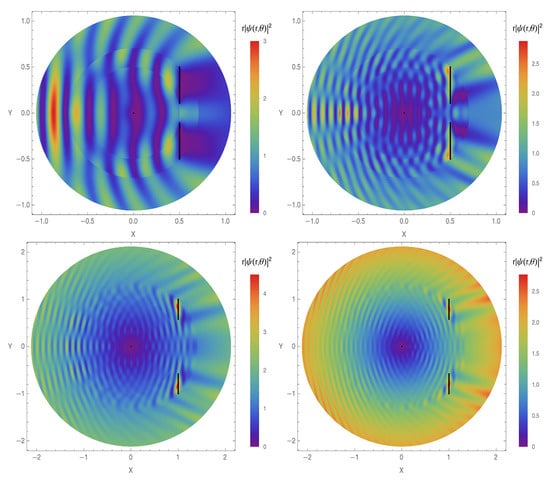
Figure 6. The probability density ${r|\Psi |}^2$ for the scattering of a plane wave by a single slit with the coupling constant $\gamma =100$. The barrier is located at a distance $x_0=1/2$ from the origin with its extremes starting from $\theta =\pi /4$ over to $\theta =-\pi /4$. The incident wave number is set to $k=4\pi$, (upper left), $11\pi$ (upper right); $8\pi$ (lower left) and $10\pi$ (lower right). The scattering incident angle is set to ${\theta }_0=0$. Black vertical segments represent the boundary walls.

In Figure 6, a single slit is defined to commence at $\theta =-\pi /15$ and to end at $\theta =\pi /15$ (Figure 6 (upper)) and to commence at $\theta =-\pi /6$ and to end at $\theta =\pi /6$ (Figure 6 (lower)). One can see the wave that passes through the slit producing a specific pattern of diffraction right after the barrier, depending on the opening size of the slit and the value of the incident momentum k. For a smaller value of the incident momentum, the barrier completely prevents the passage with the wave crossing only the slit, which is different for a higher value of the momentum. One also can notice the wave reflected by the barrier on the left side. In Figure 6 (upper), we show a smaller slit, while in Figure 6 (lower), we show a slightly larger slit for comparison, but one may notice that the effects are the same in both cases.

In Figure 7, we present the total cross-sections for the case of smaller slit (Figure 7 (left)) from Figure 6 (upper) and for the larger slit (Figure 7 (right)) from Figure 6 (lower). Similarly to the case of the line segment with no slits (see Section 2.4), one finds lower values in directions perpendicular to the incidence. From the angle $\pi /4$, one notices the increase in the absolute value of the amplitude, where secondary peaks are found; those peaks are present due to the existence of the slit. One can see that the maxima are present in the direction of incidence at $\theta =0$ and $2\pi$ (transmitted wave) and at $\theta =\pi$ (reflected wave).

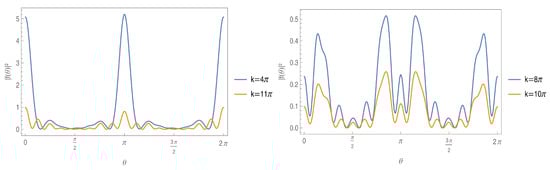
Figure 7. The differential cross-section $d\sigma /d\Omega$ for the scattering of a plane wave through a single slit for four different wave momentum values: $k=4\pi ,8\pi ,10\pi , \mathrm{and} 11\pi$, as indicated. The coupling constant is set to $\gamma =100$ and the incident scattering angle to ${\theta }_0=0$.

Figure 8 shows the total cross-section for the scattering of a plane wave by a single slit. In Figure 8 (left), we present the total cross-section as a function of k. Similar to that in Figure 7 (left),the cross-section has a series of sharp peaks for a harder barrier. When $k>18$, all three curves in Figure 7 (left) have a similar behavior. In Figure 8 (right), we present plot the total cross-section as a function of $\gamma$. The asymmetry for $k=4\pi$ is better pronounced in this case, and for $k=8\pi$, one can see, for both the repulsive and attractive waves, an almost linear (with negative slope for $\gamma <0$ and positive slope for $\gamma >0$) behavior of the total cross-section.

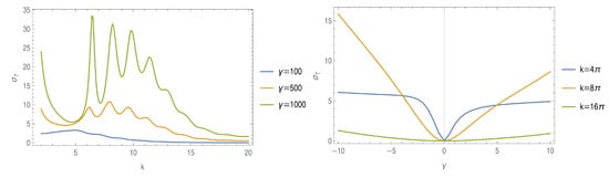
Figure 8. The total cross-section ${\sigma }_T$ for the scattering of a plane wave through a single slit as a function of the momentum k for different valus of the coupling constant $\gamma$, as indicated (left), and of the coupling constant $\gamma$ for different values of the incident momentum k, as indicated (right). The incident scattering angle is set to ${\theta }_0=0$.

4. Double Slit

Aiming the same point as that in Section 3, let us now address the double-slit scattering, just by rewriting the potential by parts (33) in order to produce the double slit, as shown in Figure 9.

Figure 9. Secant segment at $x=x_0$ with two slits, commencing at $-{\theta }_0$ and ending at ${\theta }_0$. The domain is divided into three regions: (i) interior, (ii) annular, and (iii) exterior, similar to that in Figure 1 and Figure 5.

As in Section 3, the coupling strength $\gamma$ is defined as $\gamma =1$ for the intervals with barrier and $\gamma =0$ for empty intervals. Using this configuration for solving the system, one is capable to produce the density plotsas shown in Figure 10.

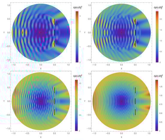
Figure 10. The probability density ${r|\Psi |}^2$ for the scattering of a plane wave by a double-slit potential with coupling constant $\gamma$ = 100. The barrier is located at a distance $x_0=1/2$ from the origin with its extremes starting from $\theta =\pi /4$ over to $\theta =-\pi /4$. The incident wave number is set to $k=8\pi$ (upper left), $10\pi$ (upper right), $14\pi$ (lower left), and $18\pi$ (lower right). The incident angle is set to ${\theta }_0=0$. Black vertical segments represent the boundary walls.

In Figure 10, the double slits are defined with ${\theta }_1=\pi /16$ and ${\theta }_2=\pi /5.8$. The value of the incident momentum k varies from $8\pi$ to $18\pi$. All images illustrate well the scattering of the plane wave by the double slit; it is possible to see how the wave crosses both slits and propagates. Here, one observes the reflection of the wave by the barrier on the left side, with different patterns from those of the plane slit; one also sees the diffraction through the slits with the wave crossing in the middle and going around the ends of the barrier, depending on the value of k, a higher or lower intensity of the wave that crosses the barrier can be noticed.

Again, as in the cases of the single segment (Section 2) and single slit (Section 3), in directions perpendicular to the incidence, one finds lower values of the differential cross-sections (Figure 11). One can also notice that there are secondary peaks due to the presence of the slits, and it can be as well noticed similar to that in the other cases considered in Section 2 and Section 3, that the larger peaks are in the directions of incidence of the waves at $\theta =0$ and $2\pi$ (transmitted wave) and at $\theta =\pi$ (reflected wave).

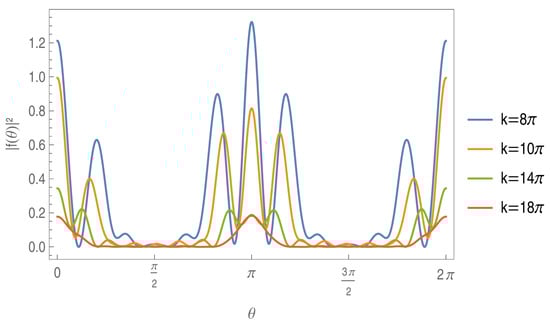
Figure 11. The differential cross-section $d\sigma /d\Omega$ for the scattering of a plane wave through two slits for four different wave momentum values: $k=8\pi ,10\pi ,14\pi , \mathrm{and} 18\pi$. The coupling constant is set to $\gamma =100$ and the incident scattering angle to ${\theta }_0=0$.

In Figure 12, we present the total cross-section for the scattering of a plane wave by a double slit as a function of the wave number (Figure 12 (left)) and coupling strength Figure 12 (right)). One can notice that the harder the barrier, the higher the cross-section for $6<k<12$. As a function of the coupling strength, one observes the two curves (for $k=8\pi \mathrm{and} 16\pi$) resembling symmetric behavior around the $\gamma =0$ axis, while the curve for $k=4\pi$ is completely asymmetric around $\gamma =0$.

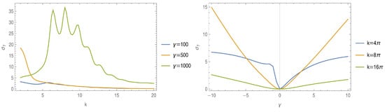
Figure 12. The total cross-section ${\sigma }_T$ for the scattering of a plane wave through two slits as a function of the momentum k for different coupling constants, as indicated (left), and of the coupling constant $\gamma$ for different momenta, as indicated (right). The incident scattering angle is set to ${\theta }_0=0$.

5. Multiple Slits Defined by Cantor Set

For a multiple-slit scattering application, it is free to choose the intervals and define them as convenient. We define a set of multiple slits based on the Cantor set. The definition of the Cantor set was originally formulated abstractly by George Cantor, studying set theory [39]. The scattering by a Cantor set has been dealt both theoretically and experimentally in the last decades [40,41,42,43]. We use the definition of a ternary set, which is constructed in an interval by an iterative process in which the middle third of a given interval is removed. A closed segment represents a Cantor set of order zero; by removing the middle third, a Cantor set of order one is obtained which represents a single slit. This process is repeated in each remaining sub-interval, thus obtaining higher-order sets, which, for the problem under consideration, produces smaller and smaller slits. This is illustrated in Figure 13.

Figure 13. Cantor set of orders 0, 1, 2, and 3 (top to bottom).

Using the Cantor set, we redefine the boundary-wall potential considered as such and reimplement the calculations using the coupling function defined by parts (33). Note that by considering more slits, more statements to define the potential, while this does not complicate the calculations more than a conditional. The results are obtained as probability densities shown in Figure 14.

Figure 14. The probability density ${r|\Psi |}^2$ for the scattering of a plane wave by multiple slits with coupling constant $\gamma =100$. The barrier is located at a distance $x_0=1/2$ from the origin with its extremes starting from $\theta =\pi /4$ over to $\theta =-\pi /4$. wave number is set to $k=4\pi$ (upper left)$11\pi$ (upper right), $8\pi$ (lower left), and $24\pi$ (lower right). The incident angle is set to ${\theta }_0=0$. Black vertical segments represent the boundary walls.

For these slits defined by the Cantor set, one can observe in Figure 14 that reflection and transmission of the wave occur differently in each image. On the right side of each image, one can see the diffraction that occurs with the wave that crosses the slits or that goes around the barrier at the ends. Notice also how a wave with low momentum k is unable to cross the smaller slits, as shown in Figure 14 (upper left) and Figure 14 (lower left); it needs to arrive with more energy at the barrier to be able to cross these smaller slits, as shown in Figure 14 (upper right) and Figure 14 (lower right), where one can see a wave with larger momentum k that is capable crossing these smaller apertures.

Figure 15 shows the differential cross-sections for multiple slits defined by the Cantor set. One notices the lowest values in the perpendicular directions. The largest values of the absolute value of the amplitude are again at $\theta =0$ and $2\pi$ (transmitted wave) and at $\theta =\pi$ (reflected wabe). For the lower-order Cantor set, one can notice fewer ridges than for the higher order, illustrating how smaller slits influence the scattering pattern.

Figure 15. Plots of the differential cross-section $d\sigma /d\Omega$ for the scattering of a plane wave through multiple slits for four different wave momentum values, $k=4\pi ,8\pi ,11\pi , \mathrm{and} 24\pi$, as indicated. The coupling constant is set to $\gamma =100$ and the incident scattering angle to ${\theta }_0=0$.

Figure 16 illustrates the total cross-sections for the Cantor set slits. From Figure 16 (left), one observes that the total cross-section is higher when the barrier has a larger coupling strength. When the total cross-section are studied as a function of the coupling strength, keeping the wave number fixed (Figure 16 (right)), the cross-section increases for both attractive and repulsive barriers.

Figure 16. The total cross-section ${\sigma }_T$ for the scattering of a plane wave through multiple slits defined over the Cantor set as a function of the momentum k for different valus of the coupling constant $\gamma$, as indicated (left), and of the coupling constant $\gamma$ for different valus of the momentum k, as indicated (right). The incident scattering angle is ${\theta }_0=0$.

One can also investigate the ratio between reflection and transmission functions. Consider for instance,

$$Q_l\left(r\right)={\displaystyle \frac{R_l\left(r\right)}{T_l\left(r\right)}}$$

(34)

in the annular region, since in the interior as well as in the exterior regions, this ratio is constant. We solved a system of linear first-order ODEs with thirty equations using Mathematica 13.3 implementation of the finite elements method (FEM). The result is illustrated in Figure 17. The curve obtained is smooth by parts because of this particular method. In the annular region, close to the inner region, i.e., for $r\le 0.56$, the reflection effect prevails, the ratio is found to exceed 1 in this region. On the other hand, when $r>0.56$, the ratio becomes less than 1, and the transmission effect prevails.

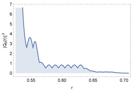
Figure 17. The square modulus $|Q_0{\left(r\right)|}^2$ of the ratio $Q_0\left(r\right)=R_0\left(r\right)/T_0\left(r\right)$ between the position-dependent reflection and transmission functions. The incident plane wave impinges upon a 3rd-order Cantor set barrier. The parameters used are $r_i=0.5018 \mathrm{and} r_f=0.7071$, respectively, for initial and final values of r, ${\gamma }_0=100, k=2\pi , \mathrm{and} {\theta }_0=0$.

6. Conclusions

Within the presented investigation, we have studied the scattering of a plane wave by four systems modeled as boundary-wall potentials: (i) a finite line segment written as a secant segment $r=x_{0}sec\left(\theta \right)$; (ii) two similarly modeled, disconnected finite lines forming a single slit; (iii) three finite line segments forming a double slit; and (iv) multiple slits constructed after Cantor’s set. We have solved the Lippmann–Schwinger equation for the delta potential barrier written over a curve and found a system of equations that were solved numerically to obtain the scattered wave function. Then, we have rewritten the potential by parts, intending to produce the slits as barriers (ii), (iii), and (iv). To this end, we have also solved the corresponding systems obtained and have found the corresponding scattered wave functions. Finally, the density plots have been presented and discussed, revealing that, for the problems considered, the reflection and transmission functions are position-dependent in an annular region.

References

- Belkić, D. Principles of Quantum Scattering Theory; IOP Publishing/Taylot & Francis Group: Oxon, UK, 2004. [Google Scholar] [CrossRef]
- Taylor, J.R. Scattering Theory: The Quantum Theory of Nonrelativistic Collisions; John Wiley & Sons, Inc.: Toronto, ON, Canada, 1972; Available online: https://cdn.preterhuman.net/texts/science_and_technology/physics/quantum_mechanics/ (accessed on 19 May 2025).
- Lippmann, B.A.; Schwinger, J. Variational principles for scattering processes. I. Phys. Rev. 1950, 79, 469–480. [Google Scholar] [CrossRef]
- Ruiz–Biestro, A.; Gutiérrez–Vega, J.C. Solutions of the Lippmann–Schwinger equation for confocal parabolic billiards. Phys. Rev. E 2024, 109, 034203. [Google Scholar] [CrossRef] [PubMed]
- Maioli, A.C.; Schmidt, A.G.M. Exact solution to Lippmann–Schwinger equation for an elliptical billiard. Phys. E Low-Dim. Syst. Nanostruct. 2019, 111, 51–62. [Google Scholar] [CrossRef]
- Maioli, A.C.; Schmidt, A.G.M. Exact solution to Lippmann-Schwinger equation for a circular billiard. J. Math. Phys. 2018, 59, 122102. [Google Scholar] [CrossRef]
- Schmidt, A.G.M.; Maioli, A.C.; Azado, P.C. Exact solution to the Lippmann–Schwinger equation for a spheroidal barrier. J. Quantit. Spectrosc. Radiat. Transf. 2020, 253, 107154. [Google Scholar] [CrossRef]
- Pereira, M.E.; Cunha, P.H.S.; Schmidt, A.G.M. Quantum scattering in a wavy circle. Phys. E Low-Dim. Syst. Nanostruct. 2024, 161, 115965. [Google Scholar] [CrossRef]
- Schmidt, A.G.M.; Pereira, M.E. Quantum refractive index for two- and three-dimensional systems. Ann. Phys. 2023, 452, 169273. [Google Scholar] [CrossRef]
- Vargiamidis, V.; Valassiades, O.; Kyriakos, D.S. Lippmann–Schwinger equation approach to scattering in quantum wires. Phys. Stat. Sol. B Basic Sol. State Phys. 2003, 236, 597–613. [Google Scholar] [CrossRef]
- Sheka, D.D.; Kravchuk, V.P.; Gaididei, Y. Curvature effects in statics and dynamics of low dimensional magnets. J. Phys. A 2015, 48, 125202. [Google Scholar] [CrossRef]
- Nishiguchi, N. Electron scattering by surface vibration in a rectangular quantum wire. Phys. E Low-Dim. Syst. Nanostruct. 2002, 13, 1–10. [Google Scholar] [CrossRef]
- Ono, S.; Shima, H. Low-temperature resistivity anomalies in periodic curved surfaces. Phys. E Low-Dim. Syst. Nanostruct. 2010, 42, 1224–1227. [Google Scholar] [CrossRef]
- Streubel, R.; Fischer, P.; Kronast, F.; Kravchuk, V.P.; Sheka, D.D.; Gaididei, Y.; Schmidt, O.G.; Makarov, D. Magnetism in curved geometries. J. Phys. D 2016, 49, 363001. [Google Scholar] [CrossRef]
- Ortix, C. Quantum mechanics of a spin-orbit coupled electron constrained to a space curve. Phys. Rev. B 2015, 91, 245412. [Google Scholar] [CrossRef]
- Andrade, F.M.; Chumbes, A.R.; Filgueiras, C.; Silva, E.O. Quantum motion of a spinless particle in curved space: A viewpoint of scattering theory. Eur. Phys. Lett. 2019, 128, 10002. [Google Scholar] [CrossRef]
- Crommie, M.F.; Lutz, C.P.; Eigler, D.M.; Heller, E.J. Quantum corrals. Phys. D 1995, 83, 98–108. [Google Scholar] [CrossRef]
- Schmidt, A.G.M.; Pereira, M.E. Analog model for scalar dynamics in a Kerr–Sen background. J. Math. Phys. 2024, 65, 122501. [Google Scholar] [CrossRef]
- Almeida, C.R.; Jacquet, M.J. Analogue gravity and the Hawking effect: Historical perspective and literature review. Eur. Phys. J. H 2023, 48, 15. [Google Scholar] [CrossRef]
- Feynman, R.P.; Leighton, R.B.; Sands, M. The Feynman Lectures on Physics; Basic Books: New York, NY, USA, 2011; Available online: https://www.feynmanlectures.caltech.edu/ (accessed on 19 May 2025).
- da Luz, M.G.E.; Lupu-Sax, A.S.; Heller, E.J. Quantum scattering from arbitrary boundaries. Phys. Rev. E 1997, 56, 2496–2507. [Google Scholar] [CrossRef]
- Kosztin, I.; Schulten, K. Boundary integral method for stationary states of two-dimensional quantum systems. Int. J. Mod. Phys. C 1997, 8, 293–325. [Google Scholar] [CrossRef]
- Goldberger, M.L.; Watson, K.M. Collision Theory; John Wiley & Sons, Inc.: New York, NY, USA, 1964; Available online: https://www.scribd.com/document/76856455/Marvin-L-Goldberger-and-Kenneth-M-Watson-Collision-Theory (accessed on 19 May 2025).
- Cavero-Peláez, I.; Milton, K.A.; Kirsten, K. Local and global Casimir energies for a semitransparent cylindrical shell. J. Phys. A 2007, 40, 3607–3632. [Google Scholar] [CrossRef]
- Gorban, M.J.; Julius, W.D.; Brown, P.M.; Matulevich, J.A.; Radhakrishnan, R.; Cleaver, G.B. First- and second-order forces in the asymmetric dynamical Casimir effect for a single δ − δ′ mirror. Physics 2024, 6, 760–779. [Google Scholar] [CrossRef]
- Oliveira, L.S.; Pereira, M.E.; Balthazar, W.F.; Schmidt, A.G.M.; Huguenin, J.A.O. Experimental study of the solutions of the Lippmann–Schwinger equation for an elliptical billiard with an intense laser beam. Phys. Lett. A 2024, 521, 129738. [Google Scholar] [CrossRef]
- Zanetti, F.M.; Lyra, M.L.; de Moura, F.A.B.F.; da Luz, M.G.E. Resonant scattering states in 2D nanostructured waveguides: A boundary wall approach. J. Phys. B 2009, 42, 025402. [Google Scholar] [CrossRef]
- Zanetti, F.M.; Vicentini, E.; da Luz, M.G.E. Eigenstates and scattering solutions for billiard problems: A boundary wall approach. Ann. Phys. 2008, 323, 1644–1676. [Google Scholar] [CrossRef]
- Azevedo, A.L.; Maioli, A.C.; Teston, F.; Sales, M.R.; Zanetti, F.M.; da Luz, M.G.E. Wave amplitude gain within wedge waveguides through scattering by simple obstacles. Phys. Rev. E 2024, 109, 025303. [Google Scholar] [CrossRef]
- Folland, G.B. Fourier Analysis and Its Applications; Brooks/Cole Publishing Company of Wadsworth, Inc.: Belmont, CA, USA, 1992; Available online: https://dokumen.pub/fourier-analysis-and-its-applications.html (accessed on 19 May 2025).
- Duffy, D.G. Green’s Functions with Applications; A Chapman & Hall Book; CRC Press/Taylor & Francis Group, LLC: New York, NY, USA, 2015. [Google Scholar] [CrossRef]
- Cohl, H.S.; Dang, T.H.; Dunster, T.M. Fundamental solutions and Gegenbauer expansions of Helmholtz operators in Riemannian spaces of constant curvature. Symmetry Itegrab.Geom. Meth. Appl. (SIGMA) 2018, 14, 136. [Google Scholar] [CrossRef]
- Pereira, M.E.; Schmidt, A.G.M. Exact solutions for Lippmann–Schwinger equation for the scattering by hyper-spherical potentials. Few-Body Syst. 2022, 63, 25. [Google Scholar] [CrossRef]
- Byron, F.W., Jr.; Fuller, R.W. Mathematics of Classical and Quantum Physics; Dover Publications, Inc.: New York, NY, USA, 1970; Available online: https://archive.org/details/mathematicsofcla00byro (accessed on 19 May 2025).
- Tricomi, F.G. Integral Equations; Dover Publications, Inc.: New York, NY, USA, 2012; Available online: https://archive.org/details/integralequation0000tric (accessed on 19 May 2025).
- Polyanin, A.D.; Manzhirov, A.V. Handbook of Integral Equations; CRC Press LLC: Boca Raton, FL, USA, 1998. [Google Scholar] [CrossRef]
- Watson, G.N. A Treatise on the Theory of Bessel Functions; Cambridge University Press: Cambridge, UK, 1995; Available online: https://www.scribd.com/doc/294269253/Treatise-on-the-Theory-of-Bessel-Functions (accessed on 19 May 2025).
- Kouri, D.J.; Vijay, A.; Hoffman, D.K. Inverse scattering theory: Renormalization of the Lippmann–Schwinger equation for quantum elastic scattering with spherical symmetry. J. Phys. Chem. A 2003, 107, 7230–7235. [Google Scholar] [CrossRef]
- Lima, E.L. Análise Real. Volume 1: Funčões de Uma Variável; IMPA: Rio de Janeiro, Brazil, 1989. [Google Scholar]
- Cherny, A.Y.; Anitas, E.M.; Kuklin, A.I.; Balasoiu, M.; Osipov, V.A. Scattering from generalized Cantor fractals. J. Appl. Crystallogr. 2010, 43, 790–797. [Google Scholar] [CrossRef]
- Hatano, N. Strong resonance of light in a Cantor set. J. Phys. Soc. Jpn. 2005, 74, 3093–3111. [Google Scholar] [CrossRef]
- Jung, C.; Scholz, H.J. Cantor set structures in the singularities of classical potential scattering. J. Phys. A 1987, 20, 3607–3617. [Google Scholar] [CrossRef]
- Rodrigo, J.A.; Alieva, T.; Calvo, M.L.; Davis, J.A. Diffraction by Cantor fractal zone plates. J. Mod. Optics 2005, 52, 2771–2783. [Google Scholar] [CrossRef]
Disclaimer/Publisher’s Note: The statements, opinions and data contained in all publications are solely those of the individual author(s) and contributor(s) and not of MDPI and/or the editor(s). MDPI and/or the editor(s) disclaim responsibility for any injury to people or property resulting from any ideas, methods, instructions or products referred to in the content. |
© 2025 by the authors. Licensee MDPI, Basel, Switzerland. This article is an open access article distributed under the terms and conditions of the Creative Commons Attribution (CC BY) license (https://creativecommons.org/licenses/by/4.0/).