Statistical Scrutiny of Particle Spectra in ep Collisions


1
Department of Technology, Savitribai Phule Pune University, Pune 411007, India
2
Department of Physics, Panjab University, Chandigarh 160014, India
3
Department of Physics, Amity University, Mohali 140306, India
*
Author to whom correspondence should be addressed.
Physics 2021, 3(3), 757-780; https://doi.org/10.3390/physics3030047
Submission received: 21 April 2021
/
Revised: 20 August 2021
/
Accepted: 23 August 2021
/
Published: 8 September 2021
(This article belongs to the Special Issue Statistical Approaches in High Energy Physics)
Abstract
:Charged particle multiplicity distributions in positron–proton deep inelastic scattering at a centre-of-mass energy = 300 GeV, measured in the hadronic centre-of-mass frames and in different pseudorapidity windows are studied in the framework of two statistical distributions, the shifted Gompertz distribution and the Weibull distribution. Normalised moments, normalised factorial moments and the H-moments of the multiplicity distributions are determined. The phenomenon of oscillatory behaviour of the counting statistics and the Koba-Nielsen-Olesen (KNO) scaling behaviour are investigated. This is the first such analysis using these data. In addition, projections of the two distributions for the expected average charged multiplicities obtainable at the proposed future ep colliders.
1. Context and Introduction
Ever since the discovery of quarks and gluons, the search for their composites forming new particles in the form of leptons and hadrons has driven high energy physicists to strive for higher and higher energy regimes in pursuit of new exotic particles. Unprecedented and cutting edge technological developments, combined with scientific expertise have pushed the energy frontier to new levels. This made possible the discovery of Higgs boson at the Large Hadron Collider (LHC) [1] at CERN in recent years. During the past four decades, beam accelerators of mammoth sizes have been built for delivering the highest possible collision energies, necessary for discovering new physics. Some of the extraordinary particle accelerators include LHC, the Large Electron–Positron Collider (LEP) [2], the Hadron–Electron Ring Accelerator (HERA) [3], the Proton–Antiproton Collider (Tevatron) [4] and the Relativistic Heavy-Ion Collider (RHIC) [5]. While colliders make the collisions of a given kind of particles possible, the collision energy results into producing a large number of particles of different types. In order to record the outcome of the particle collisions, the most complex high energy particle detectors have been designed. These giant particle detectors are engaged to track and record these particles produced in collisions. Interestingly, the information of the output of a collision, which can be obtained from the detector is rather limited in terms of directly observable quantities. Some directly measurable quantities include the number of particles produced, the charge of a particle, the angle at which a particle is produced and its momentum and energy. All other properties of the particle have to be inferred by indirect methods.
The first and foremost physical observable in any high energy interaction is a count of the particles produced. Charged particles are directly observable. Neutral particles must be detected from their decay products. Charged particles are measured in full or sliced phase space. Majority of the charged particles produced are pions, protons and kaons. The distribution of charged particles is studied systematically to probe into the production dynamics and any embedded correlations. Definite trends of the average number of particles produced, dependence on collision energy and phase space, form an interesting subject of study. Several theoretical, phenomenological and statistics-inspired approaches are adopted to understand and explain the observations of the experiments. One of the earliest efforts to understand the behaviour of probability of particle production led to the observation of a scaling behaviour, known as the Koba–Nielsen–Olesen (KNO) scaling [6,7]. Efforts to use probability distribution functions (PDF) in terms of statistical discrete distributions, such as binomial, Poisson, Bernoulli, negative binomial and multinomial [8] etc. have produced results applicable at different collision-energies. One of the most consistent description of particle production has been provided by the negative binomial distribution (NBD) [9]. Some of the statistical distributions and their modified forms which have been widely used are NBD [9,10], Gamma distribution [11], Lognormal distribution [12], Tsallis distribution [13,14] and the Weibull distribution (WD) [15,16,17]. Biró et al. [18] and Shen et al. [19] have studied particle production in heavy-ion collisions in terms of Tsallis non-extensive entropy in relation to the temperature T, and the non-extensivity parameter q. It has been extensively used to study the particle spectra produced in different types of collisions, from ee, pp, pA to AA to understand the mechanism of particle production [20,21,22,23,24,25,26].
In the present study, investigation of the charged hadronic multiplicity in ep collisions at HERA is made in terms of the shifted Gompertz distribution (SGD) and the Weibull distribution. The application of these distributions are made to study multiplicity distributions of charged particles produced in ee, pp, p and the hadron−nucleus (hA) collisions at different center-of-mass (c.m.) energies in full phase space and also in restricted phase space windows. The results of the study are published in [27,28,29,30,31,32]. The present work is the first attempt to analyse the data from different hadronic energy regions in the deep inelastic scattering (DIS) at the HERA.
To date, only one collider namely HERA was built to provide ep collisions at different energies. Number of future high energy ep colliders are being planned to extend the kinematic reach of an electron to probe the inner structure of a proton. Using the SGD, the behaviour of average charged multiplicity at HERA is studied and utilised to make predictions for the particle production at energies achievable at the future accelerators.
2. The Data from HERA and Kinematical Variables
The first ever constructed electron–proton storage ring, the HERA, was located at the DESY laboratory in Hamburg, Germany. It was 6.3 km in circumference and had four interaction regions which housed the experiments H1, ZEUS, HERMES, and HERA-B. Of the four experiments, H1 and ZEUS recorded the collisions of e and proton beams. At the interaction points, beam of positrons having 27.5 GeV energy were collided with 820 GeV protons at a c.m. energy of 300 GeV. HERA was an asymmetric accelerator and its unique kinematics made it possible to observe the hadronic recoil, in addition to the access to weak neutral-and-charged currents. Two of the detectors H1 and Zeus, recorded the outcome of positron collisions with protons, at the HERA storage ring at DESY. The H1 data [33] under scrutiny were collected during the 1994 running period, corresponding to an integrated luminosity of 1.3 pb.
In the present study, corrected multiplicity distributions are studied in different intervals of pseudo-rapidity, , and in the intervals of the c.m. energy of hadronic system, W. Multiplicity distributions analysed are in the kinematic regions of W: 80 → 115, 115 → 150, and GeV for charged hadrons with pseudo-rapidity in different domains with = 2, 3, 4, 5, i.e., in increasing size of pseudo-rapidity window. Pseudo-rapidity is defined as , where is the angle between the hadron momentum and the positive direction of the beam axis. For this analysis, is measured in the current hemisphere and denoted as , with being the angle between the hadron momentum and the direction of the virtual photon in the p rest system.
Scattering of a lepton from a proton can be viewed as the elastic scattering of the lepton from a quark or anti-quark inside the proton, as illustrated in Figure 1.
Denoting the initial four-momentum of the lepton as k, final four-momentum of the lepton as , initial four-momentum of the proton as p, fraction of the proton-momentum carried by the struck quark as x and the final four-momentum of the hadronic system as , following invariant variables can be defined:
where s is the center-of-mass energy squared, t is the four-momentum transfer squared between the proton and the final state hadronic system, y is the inelasticity of the scattered lepton and is the invariant mass squared of the final state hadrons. The energy momentum conservation demands are:
The multiplicity distributions are studied in the virtual-boson proton (p) rest system, the hadronic centre-of-mass frame. Data for probability distributions in different and W bins, have been taken from H1 experiment [33]. As reported in this paper, for each multiplicity, n, the statistical uncertainties were taken into account for the finite number of events in the data and in the samples generated by using several Monte Carlo (MC) event generators which include the DJANGO and the LEPTO programs to model the hadronic final states [34,35]. They were calculated by using the Monte Carlo sampling procedure to ensure the propagation of sampling fluctuations and statistical correlations, described therein.
3. Statistical Methods of Analysis
3.1. Scaling
In order to establish the energy-independence of multiplicity distribution, Koba et al. [6,7] proposed that at very high energy the probability of producing n particles in a certain collision process should exhibit the scaling relation:
with the average multiplicity of particles produced at collision energy . This behaviour was known as KNO-scaling. This hypothesis has been widely studied and confirmed in different types of collisions. Deviation from KNO-scaling was first observed in proton−proton collisions at the Intersecting Storage Ring (ISR) energies [36]: = 30.4 to 62.2 GeV. With more data becoming available from different collider experiments at different energies, in varying intervals of phase space and for different types of collisions, the scaling behaviour is still being studied. After the observation of KNO-scaling violation, NBD became the most widely used distribution to describe the multiplicities. Almost every experiment, designed to study collisions of any kind: ee, ep, p, pp, hA and AA used NBD to understand the mechanism of particle production.
3.2. Parametric Distributions
Study of the multiplicity distributions by the H1 collaboration [33], showed that the Log-normal distribution (LND) [37,38] gives a reasonably accurate description of the data, in particular in the smallest domain. However, the quality of the fits deteriorated in larger domains. The NBD fits were acceptable in the smallest domain but became progressively worse for larger intervals. The two distributions were found to differ strongly for low multiplicities.
The success of NBD remained unchallenged by showing its ability to describe almost all the data available at different energies until, the multiplicity measurements from the UA1 collaboration [39] and the UA5 collaboration [40,41] on the p collisions at 540 GeV revealed the NBD violation. The multiplicity distribution showed a shoulder structure in the probability versus n dependence at this energy. In ee annihilation at = 91 GeV at the LEP, the multiplicity distribution also exhibited a prominent shoulder structure at intermediate n values. Thus, LND and NBD both were unable to describe the distributions. The shoulder was the most prominent in single hemisphere distributions [42,43]. However, the H1 measurements showed no evidence for a shoulder structure of the type. Nevertheless, these parametric forms continued to be useful for phenomenological studies. Since then, several new probability functions have been proposed and used for the description of multiplicities.
The SGD [27] is the distribution of the largest of two independent random variables one of which has an exponential distribution with parameter b and the other has a Gumbel distribution, also known as log-Weibull distribution with parameters t and b. In its original formulation the distribution was expressed referring to the Gompertz distribution instead of the Gumbel distribution but, the Gompertz distribution is a reverted Gumbel distribution. SGD finds application to problems in statistics, mathematics, computer science, social networks, in the market research, diffusion theory, and forecasting etc. A possibility to apply this distribution to the statistical phenomena in high energy physics, motivated us to use it for the description of multiplicity distributions. SGD with two non-negative fit parameters is thus proposed to be used for understanding the particle production in sub-nuclear particle collisions.
Let N be a random variable following SGD with parameters b and t, where is a scale parameter and is a shape parameter. The probability density function (PDF) of N is
The distribution can be characterised by the maximum of two independent random variables with Gompertz distribution (parameters and ) and exponential distribution (parameter ). For , the SGD approximates to an exponential distribution with mean = . A thorough interpretation of SGD is detailed in references [44,45]. In the paper by Jiméne Torres and Jodrá [46], it is emphasised that the computation of moments is rather complicated. Even for the first and second moment, the integrals involved to obtain to calculate mean and variance do not have closed-form solution in terms of simple functions. However, explicit expressions for the moments of orders 1 and 2 were obtained by the authors. Furthermore, Bemmaor [44] gave implicit formulae to compute the expectation and variance of the distribution. The following expressions for mean and the moments are thus adopted from these references.
Mean of the distribution:
and
where E is the expectation function. SGD has been recently studied in hadronic and leptonic interactions. The aim of this paper is to extend its applicability to high energy deep inelastic scattering in different regimes of W and . The mean of the distribution as given in Equation (11) is expected to approximate the mean of the experimental distribution, .
Another distribution was used by S. Dash et al. [16,17] for the description of multiplicity data in ee and p collisions at different energies. WD is a continuous probability distribution which can take many shapes. It can also be fitted to non-symmetrical data. WD has two parameters. The characteristic value in a standard Weibull function is known as scale parameter. The second parameter of the distribution , is the shape parameter.
The probability density function of a Weibull random variable is
Mean of the distribution can be calculated from the following equation:
Various steps to obtain the Equation (14) are given in Appendix A.
For a multiplicity distribution, the normalised moments , normalised factorial moments , normalised factorial cumulants and ratio of the two, moments are defined as
where is the -charged particle probability and q is the rank of the moment.
In the specific case of SGD, normalized moments () and normalized factorial moments () are defined below, with n as values of X:
where q is a natural number ranging from 1 to ∞. The mean value (E[X]) of SGD is given by
The higher order moments () can be found by using the moment generating function of the SGD [[b,t],m]
Higher order factorial moments () can be found by using the generating function of SGD [[b,t],m]
where:
- (i)
- ≈ 0.5772156 is the Euler–Mascheroni constant.
- (ii)
- [s] the Euler Gamma function and the incomplete Gamma function are defined as
- (iii)
- is a Generalized Hyper-geometric function.
SGD and WD both are continuous distributions. The question arises, are this type of distributions suitable to describe discrete multiplicity data? The usage of continuous distributions such as, e.g., Gamma, lognormal, Weibull distributions to study the multiplicity data in high energy physics has been adopted in several studies. Tsallis distribution, a statistical distribution based on q-exponential and q-logarithm functions has also been widely used. Recently Weibull distribution has been introduced and used for the multiplicity data from several experiments. Multiplicity data constitute discrete data sets. In order for any continuous distribution to be used to describe the discrete data, a continuity correction may be used. In a high energy experiment, one observes the number of particles produced in a collision. This number varies between 0 and a maximum value, n. Suppose one needs to compute the probability of obtaining 10 particles. While the discrete random variable can have only specified value (10 in this case), a continuous random variable used to approximate it could take on any values within an interval around this value. In this case it varies by one unit, . With a continuous distribution, the probability of obtaining a particular value of a random variable is zero. But when it is used to approximate a discrete distribution, a continuity correction can be employed so that one can approximate the probability of a specific value of the discrete distribution. As shown in [47,48], for an underlying continuous random variable X, the discrete analogue Y is given by:
where the parameter is so chosen that the first two raw moments of X and Y remain close.
4. Analysis of the Data
The two distributions SGD and WD, described in Section 2, are fitted to the ep collision data collected by the H1 detector. The best fits are obtained by using the minimisation of technique from the CERN’s analysis framework, ROOT6.18.
4.1. The SGD and WD Fits
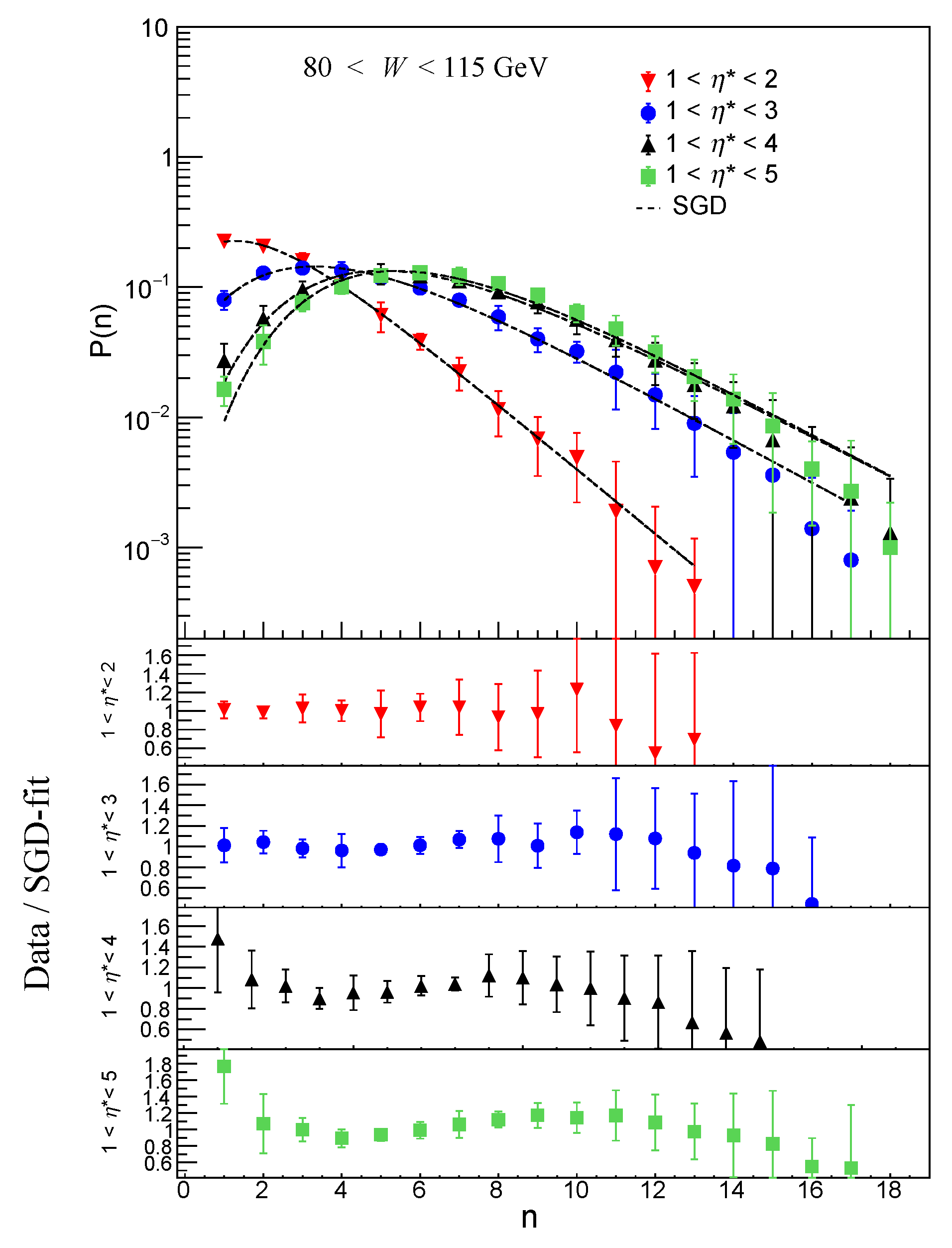
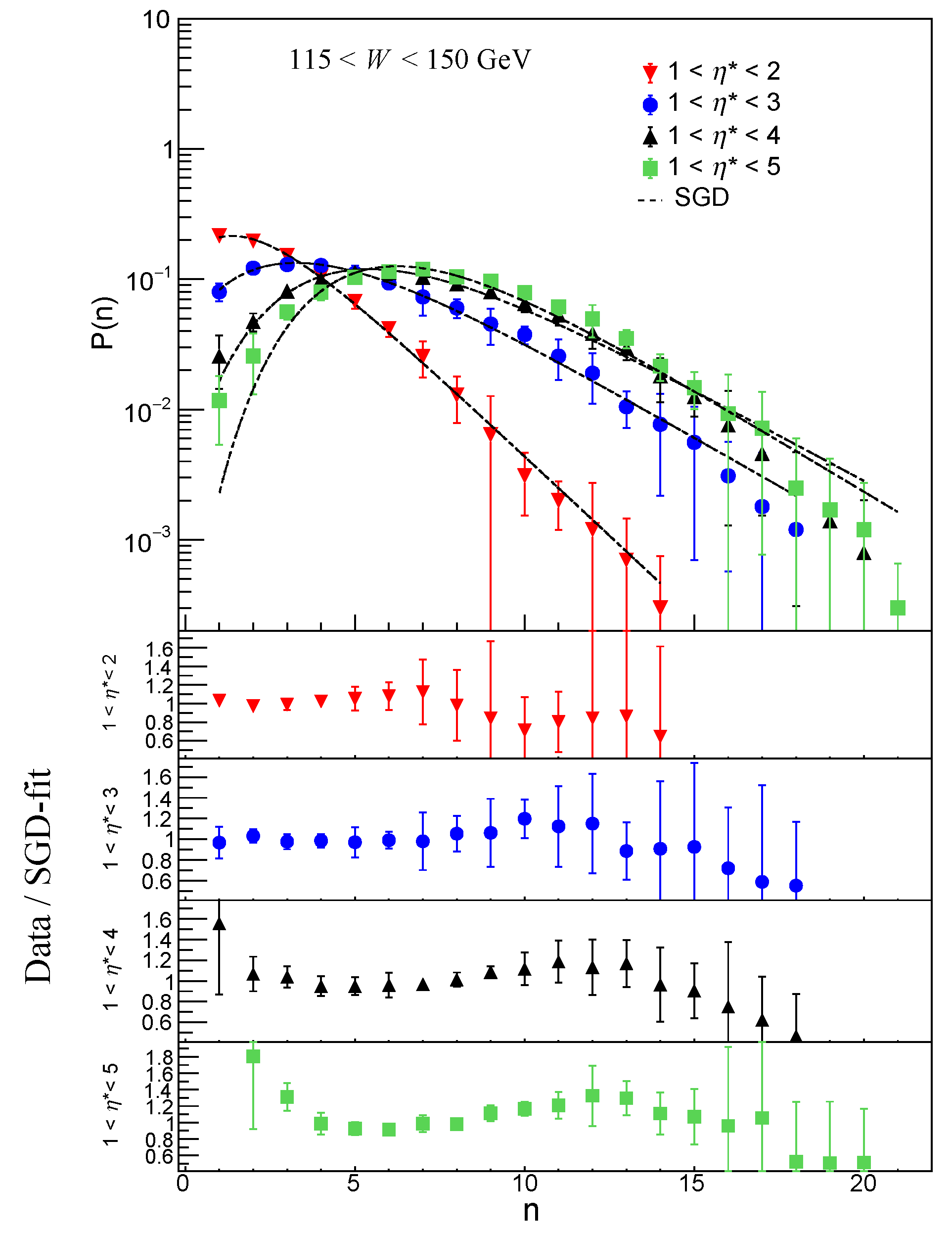
Figure 2, Figure 3, Figure 4 and Figure 5 show the multiplicity distributions fitted with SGD, Equation (11), in different and W intervals and for W in the intervals, 80 < W < 115 GeV, 115 < W < 150 GeV, 150 < W < 185 GeV, 185 < W < 220 GeV. The figures also show the data versus SGD-fit ratio plots enabling an understanding of the goodness of the fit. Parameters of the fits and ndf (number of degrees of freedom) for all the fits are given in Table 1. The parameters measured from the distributions relate to the scale and shape of the distributions. The tail of the distribution determines the maximum number of particles produced in an interaction. The scale of each distribution is studied in different phase space regions and its dependence on the energy. Similarly, shape parameter affects the shape of the distribution. It connects to the higher moments such as 3rd moment (skewness) and 4th moment (Kurtosis) of the distribution. If the distribution is left skewed, the probability of producing events with small multiplicity decreases and vice versa for the case when it is right skewed. This affects the mean of the distribution, the average charged particle multiplicity in this analysis.
Figure 6, Figure 7, Figure 8 and Figure 9 show the WD defined in Equation (A1) fitted to the data in different and W intervals. The figures also show the data versus WD-fit ratio plots which help in understanding the goodness of the fit. Parameters of the fits and /ndf are given in Table 2. Optimised values of the parameters determine the fit between the data and the function.
Some experimental distributions are studied by using the continuous form of SGD and WD and also by calculating the continuity correction of = 0.5 as shown in Equation (27). No appreciable differences in the data versus distributions fits are found. A detailed study of this comparison by using data from several collider experiments will soon be published. Generating discrete analogues of continuous distributions is well explained in the references [47,48].
4.2. Normalised and Factorial Moments of Multiplicity Distributions
Evaluation of successive moments of a multiplicity distribution relates to the shape and scale of the distribution. The moments can be studied as a function of the collision energy and to check the validity of KNO scaling. Multiplicity distribution is expected to demonstrate the scaling property. So that the Multiplicity distribution is expected to lead to a common scaled behaviour when calculated as as a function of . Higher-order moments and the cumulants are the precise tools for predicting the correlations amongst the charged particles produced in a collision. Deviation w.r.t. independent and uncorrelated production of particles can be observed effectively by measuring factorial moments. Broadening of the distribution beyond the expectation of Poisson distribution, indicates the presence of particle correlations, with the values becoming greater than unity.
Figure 10 and Figure 11 show the normalized moments for q = 2, 3, 4, 5 calculated from the SGD and WD fits for different W ranges in four pseudorapidity intervals, 1 < < 2, 1 < < 3, 1 < < 4 and 1 < < 5. Corresponding values obtained from the fits are given in Table 3 and Table 4. Furthermore, values of the moments derived from the data are given in Table 5.
Figure 12 and Figure 13 show the normalized factorial moments for q = 2, 3, 4, 5 calculated from the SGD and WD fits to the distributions at different W and in different pseudorapidity intervals. Corresponding values obtained from the fits are given in Table 3 and Table 4. The values of the moments derived from the data are given in Table 5.
4.3. Moments of Multiplicity Distributions
The first results on the moments are presented in this section. Figure 14 shows the moments versus q variation calculated from the data and compared with SGD and WD distributions in different bins. A good agreement with the data can be observed. Results are shown for three bins: , and . The bin with has very low statistics and hence is not included.
4.4. Average Charged Particle Multiplicity
The average charged particle multiplicities for the interactions at of 300 GeV have been calculated using the distributions obtained from the SGD and WD fit models, for all . These values obtained are found to be in good agreement with the H1 experimental values, as shown in Table 6. The values obtained from the SGD and WD models in the pseudorapidity interval are fitted with a linear function of ln using the relation
Values of the parameters and , obtained for the SGD model are , , and for the WD model are , respectively. The ndf for SGD and WD fits are 3.35/2 and 0.1/2, respectively.
5. Projections of for the Proposed Future Colliders
The proposed future high energy ep colliders, the Large Hadron Electron Collider LHeC [49], Future Circular Collider (FCC)-eh [50] and a Very High energy electron–proton collider (VHep) [51,52] aim to extend the kinematic reach of electron probe inside the proton. The colliding beam energies and c.m. energies expected from these colliders are listed in Table 7.
The increased c.m. energies that can be achieved at the proposed future ep colliders, are projected to be many orders higher than the HERA energies. This will facilitate to probe precisely the structure of proton, perform other standard tests of quantum chromodynamics (QCD) and to look for the signatures of physics beyond Standard Model (BSM) in a whole new kinematic region currently non-achievable.
Figure 15 shows the expected from SGD and WD models, calculated from Equation (28), at different W for the interval , covering the ranges offered in the past by the H1 detector at HERA and all the other three proposed future high energy ep colliders. The blue and grey bands are uncertainty bands on the SGD and WD central fit values, respectively. Reach of the proposed future ep colliders in terms of W are depicted in Figure 15 and also shown are the values of expected at these very high energies.
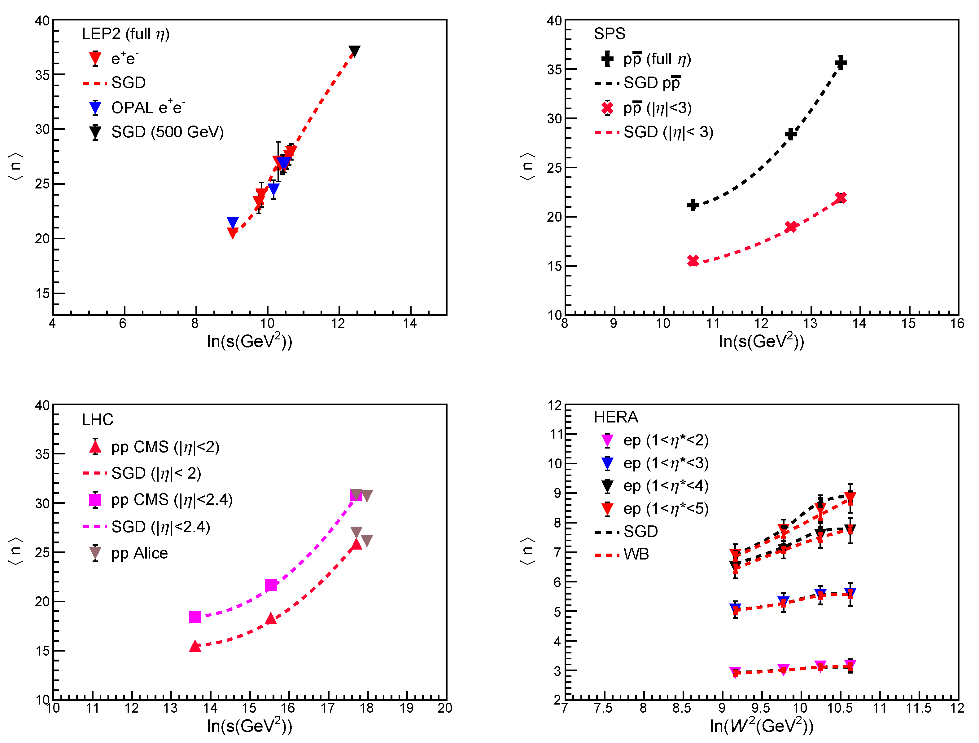
Figure 16 shows the dependence on for four different types of collisions: ee [53,54,55,56,57] in the full range, p [41,58] in two phase space windows (the full and ), pp [59,60,61] collisions in the and windows and ep in different ranges. Square of c.m. energy available for particle production s is represented by in case of ep collisions. In each of the three cases, dashed lines represent the SGD predictions. For these collisions the analyses in terms of SGD were presented in our earlier publications. However the versus dependence was not studied. From Figure 16 it may be observed that the data agree with the SGD predictions, and is more than at full width in the common . It is also observed that in the region for pp and corresponding region for ep, the is very large for the pp/p collisions as compared to the ep collisions. Roy et al. [62], in a recent publication, studied dependence on energy for ee, ep, and p collisions, to search for scaling properties of average multiplicity and pseudorapidity density. They made a similar observation that > > at each value of . Their analysis led to a common fit to the data from all different types of collisions, as shown in Figure 1 of the paper [62]. In ep data at HERA, the dependence on increases linearly with the increasing size of pseudorapidity window.
6. Results and Conclusions
The statistical behavior of charged particle multiplicity in the hadronic final state of deep inelastic ep scattering in the p c.m. energy range, 80< W< 220 GeV is investigated. From the shapes of the Multiplicity distributions in Figure 2, Figure 3, Figure 4, Figure 5, Figure 6, Figure 7, Figure 8 and Figure 9, it may be observed that for both SGD and WD the high-multiplicity tails of the distributions increase faster with increasing energy than the low-multiplicity part. The same trend can be observed with broadening of pseudorapidity interval. This feature points towards a possible beginning of the KNO scaling violation in high energy region. An investigation of multiplicity distribution in reference [33], also concluded that the property of KNO scaling remains valid in DIS at HERA for small and for large pseudorapidity intervals, but not for intermediate size intervals.
The data/fit ratio plots show disagreement between the data and the SGD fit values in lower multiplicity region, particularly for in the two largest intervals: 1 < < 4 and 1 < < 5 for all . Comparison of ratio plots in the WDs in Figure 6, Figure 7, Figure 8 and Figure 9 show good agreement with the data within the limits of error. SGD shows some disagreement in the low multiplicity region. This is because the data suffers from low statistics in this region. Similar observation was reported in the paper by H1 collaboration [33]. With LND and NBD functions it was found that large n tail of the experimental distributions is well described but deviations occur for small multiplicities.
It may be observed that both normalised moments, , and normalised factorial moments, , computed from the SGD and WD fits, agree well with the values obtained from the data. However, due to limited statistics, values calculated from the data have large errors. At fixed W the moments decrease as window increases in size from 1 < < 2 to 1 < < 5. This implies widening of multiplicity distribution in the KNO form. Broadening of the distribution results in the values becoming greater than unity. Thus, beyond the expectation of KNO distribution, it indicates the presence of particle correlations.
From the Figure 10, Figure 11, Figure 12 and Figure 13 and the values given in the Table 3, Table 4 and Table 5, it is observed that and remain roughly constant over the W range between 80 GeV and 220 GeV, for the same pseudorapidity windows. and show a marginal increase with increasing W.
Exact KNO scaling implies that moments , are independent of W. Thus, moments in the smallest and the largest pseudorapidity windows show little dependence on energy, thus exhibiting approximate KNO scaling. The intermediate size windows point towards the violation of KNO scaling. This observation is consistent with observation at HERA in DIS data on multiplicity distributions [63,64].
The factorial moments , show little W-dependence, within limits of errors, while , show a small increase with increasing W. Uniform constancy of the factorial moments establishes KNO scaling.
In the earlier paper [32], the moments of ee, pp and p collisions were studied by us and the violation of KNO scaling was shown, as observed for higher moments in the measured data. At higher energies, particularly at the LHC energies, the moments strongly are dependent on the energy. It was observed that the values for both the normalised moments, , as well as normalised factorial moments, , computed from the SGD fits were in agreement with the values obtained from the data. Both types of moments were found to decrease with widening of the pseudorapidity window for both pp (for ) and p (for ).
The ratio of cumulants to factorial moments is defined as moments. A special oscillation pattern is observed in the shape of multiplicity distribution, when analysed in terms of moments varying with the rank of the moment q. Moments grow very rapidly with q, but the growth cancels in their ratio. This makes the graphical representation of better understood. Details are well described in references [65,66,67,68].
Study of dependence of moments on the rank of moment q, shows the oscillatory behaviour, with first minimum occurring around 5. This behaviour was explained well within the theory of perturbative QCD [69,70,71]. In the earlier paper by us [29], hadronic multiplicities in ee, pp and p collisions and moments were studied, by using SGD. For different species of the colliding particles, similar oscillations in the moments were observed in different pseudorapidity windows and also in the forward region. Furthermore, the shape of the multiplicity distributions analyzed in terms of the moments was found to reveal quasi-oscillations.
In the present study, analysis of multiplicity distributions in ep data, using SGD and WD, shows similar oscillations in moments. The behaviour of moments in different and in different W ranges is studied. The shape of the multiplicity distribution (in every W range) analyzed in terms of the moments was found to show the quasi-oscillations in the regime of large q values. The perturbative QCD also predicts, a negative first minimum near 5 and expected quasi-oscillations of about zero for larger values of q.
Overall, the results from analysis of different types of moments are compatible with the results obtained earlier from ee, pp and p collisions at different energies and in different phase space windows.
It may be observed that SGD and WD both describe the data well and with a minimum around 5, although WD reproduces the data more closely. The dependence of on the rank of moment, q in all windows shows a steep descent to a minimum value around q = 4–5. Beyond the minimum it tends to flatten out for higher q. A more regular quasi-oscillations about zero can be seen in the pseudorapidity windows and . These observations follow closely the predictions from QCD and also the next-to-next-to-leading logarithm approximation (NNLLA) of perturbative QCD.
The mean charged multiplicity , calculated from the ep data, SGD and WD fits in different intervals of W and different pseudorapidity windows, are in agreement within errors. The dependence on W follows a linear dependence as ln. Using this dependence, values at the future, very high energy ep colliders are predicted.
The dependence of on for three different types of collisions: ee in the full range, p in two phase space windows (the full and ), and pp collisions in the and windows has been studied. It may be observed that the data agree with the SGD predictions and is more than at full width in the common . It is also observed that in the pseudorapidity region for pp and corresponding region for ep, the is very large for the pp/p collisions as compared to the ep collisions. This observation agrees with the observation made in a paper by Roy et al. [62] that > > at each value of . The increases linearly with with the increasing size of pseudorapidity window in ep data at HERA.
Author Contributions
Both authors contributed equally to the conceptualization, methodology, data analysis, manuscript preparation, presentation of results and conclusions. All authors have read and agreed to the published version of the manuscript.
Funding
Author R.A. received funding from the Department of Science and Technology, Government of India under DST INSPIRE Faculty grant.
Data Availability Statement
For the present analysis, data sets analysed can be found at the site, https://www.hepdata.net/record/ins422230, accessed on 21 January 2021.
Acknowledgments
The author R. Aggarwal is grateful to the Department of Science and Technology, Government of India, for the INSPIRE faculty grant.
Conflicts of Interest
The authors declare no conflict of interest.
Appendix A
Derivation of Equation (14).
The probability density function of a Weibull random variable is;
To find mean :
Let
Comparing with a standard gamma function:
References
- The Large Hadron Collider. Available online: https://home.cern/science/accelerators/large-hadron-collider (accessed on 15 February 2021).
- The Large Electron-Positron Collider. Available online: https://home.cern/science/accelerators/large-electron-positron-collider (accessed on 15 February 2021).
- HERA. Available online: https://www.desy.de/research/facilities_projects/hera/index_eng.html (accessed on 20 February 2021).
- Tevatron. Available online: https://www.fnal.gov/pub/tevatron/tevatron-accelerator.html (accessed on 20 February 2021).
- Relativistic Heavy Ion Collider. Available online: https://www.bnl.gov/rhic/ (accessed on 20 February 2021).
- Koba, Z.; Nielsen, H.B.; Olesen, P. Scaling of multiplicity distributions in high energy hadron collisions. Nucl. Phys. B 1972, 40, 317–334. [Google Scholar] [CrossRef]
- Gaździcki, M.; Szwed, R.; Wrochna, G.; Wróblewski, A.K. Scaling of multiplicity distributions and collision dynamics in e+e− and pp interactions. Mod. Phys. Lett. A 1991, 6, 981–992. [Google Scholar] [CrossRef]
- Prosper, H.B. Practical Statistics for Particle Physicists. arXiv 2016, arXiv:1608.03201. [Google Scholar]
- Carruthers, P.; Shih, C.C. The phenomenological analysis of hadronic multiplicity distributions. Int. J. Mod. Phys. A 1987, 2, 1447–1547. [Google Scholar] [CrossRef]
- Giovannini, A.; Ugoccioni, R. Clan structure analysis and qcd parton showers in multiparticle dynamics: An intriguing dialog between theory and experiment. Int. J. Mod. Phys. A 2005, 20, 3879–3999. [Google Scholar] [CrossRef] [Green Version]
- Urmossy, K.; Barnaföldi, G.G.; Birò, T.S. Microcanonical Jet-fragmentation in proton-proton collisions at LHC Energy. Phys. Lett. B 2012, 718, 111–118. [Google Scholar] [CrossRef] [Green Version]
- Szwed, R.; Wrochna, G.; Wróblewski, A.K. Genesis of the lognormal multiplicity distribution in the e+e− collisions and other stochastic processes. Mod. Phys. Lett. A 1990, 5, 1851–1869. [Google Scholar] [CrossRef]
- Tsallis, C. Possible generalization of Boltzmann-Gibbs statistics. J. Stat. Phys. 1988, 52, 479–487. [Google Scholar] [CrossRef]
- Agüiar, C.E.; Kodama, T. Nonextensive statistics and multiplicity distribution in hadronic collisions. Phys. Stat. Mech. Appl. 2003, 320, 371–386. [Google Scholar] [CrossRef] [Green Version]
- Weibull, W.; Weibull, A. Statistical distribution function of wide applicability. J. Appl. Mech. 1951, 18, 293–297. [Google Scholar] [CrossRef]
- Sadhana, D.; Nandi Basanta, K.; Priyanka, S. Weibull model of multiplicity distribution in hadron-hadron collisions. Phys. Rev. D 2016, 93, 114022–114037. [Google Scholar]
- Sadhana, D.; Nandi Basanta, K.; Priyanka, S. Multiplicity distributions in e+e− collisions using Weibull distribution. Phys. Rev. D 2016, 94, 074044–074049. [Google Scholar]
- Biró, T.S.; Barnaföldi, G.G.; Ván, P. Quark-gluon plasma connected to finite heat bath. Eur. Phys. J. 2013, 49, 110–114. [Google Scholar] [CrossRef] [Green Version]
- Shen, K.; Barnaföldi, G.G.; Biró, T.S. Hadronization within the non-extensive approach and the evolution of the parameters. Eur. Phys. J. 2019, 55, 126–144. [Google Scholar] [CrossRef] [Green Version]
- Gabór, B.; Barnaföldi, G.G.; Sándor, B.T. Tsallis-thermometer: A QGP indicator for large and small collisional systems. J. Phys. G Nucl. Part Phys. 2020, 47, 105002. [Google Scholar]
- Bhattacharyya, T.; Khuntia, A.; Sahoo, P.; Garg, P.; Pareek, P.; Sahoo, R.; Cleymans, J. The q-statistics and QCD Thermodynamics at LHC. Acta Phys. Pol. B Proc. Supp. 2016, 9. [Google Scholar] [CrossRef] [Green Version]
- Bhattacharyya, T.; Cleymans, J.; Khuntia, A.; Pareek, P.; Sahoo, R. Radial Flow in Non-Extensive Thermodynamics and Study of Particle Spectra at LHC in the Limit of Small (q − 1). Eur. Phys. J. A 2016, 52, 30. [Google Scholar] [CrossRef]
- Khuntia, A.; Tripathy, S.; Sahoo, R.; Cleymans, J. Multiplicity Dependence of Non-extensive Parameters for Strange and Multi-Strange Particles in Proton-Proton Collisions at = 7 TeV at the LHC. Eur. Phys. J. A 2017, 53, 103. [Google Scholar] [CrossRef] [Green Version]
- Zheng, H.; Zhu, L. Can Tsallis distribution fit all the particle spectra produced at RHIC and LHC? Adv. High Energy Phys. 2015, 2015, 180491. [Google Scholar] [CrossRef] [Green Version]
- Cleymans, J.; Worku, D. The Tsallis Distribution in Proton-Proton Collisions at = 0.9 TeV at the LHC. J. Phys. G 2012, 39, 025006. [Google Scholar] [CrossRef]
- Rutuparna, R.; Khuntia, A.; Sahoo, R.; Cleymans, J. Event multiplicity, transverse momentum and energy dependence of charged particle production, and system thermodynamics in pp collisions at the Large Hadron Collider. J. Phys. G Nucl. Part Phys. 2020, 47, 055111. [Google Scholar]
- Chawla, R.; Kaur, M. A new distribution for multiplicities in leptonic and hadronic collisions at high energies. Adv. High Energy Phys. 2018, 2018, 5129341. [Google Scholar] [CrossRef]
- Kaur, A.; Aggarwal, R.; Kaur, M. Investigation of particle production in h–A collisions using statistical distributions. Int. J. Mod. Phys. E 2021, 30, 2150007. [Google Scholar] [CrossRef]
- Aggarwal, R.; Kaur, M. Charged particle production in pp collisions at = 8, 7 and 2.76 TeV at the LHC-a case study. Int. J. Mod. Phys. E 2021, 30, 2150005. [Google Scholar] [CrossRef]
- Aggarwal, R.; Kaur, M. Comparative study of charged multiplicities and moments in pp collisions at = 7 TeV in the forward region at the LHC. Phys. Rev. D 2020, 102, 054005. [Google Scholar] [CrossRef]
- Aggarwal, R.; Kaur, M. Compelling evidence of oscillatory behaviour of hadronic multiplicities in the shifted Gompertz distribution. Adv. High Energy Phys. 2020, 2020, 5464682. [Google Scholar] [CrossRef] [Green Version]
- Singla, A.; Kaur, M. Charged-Particle multiplicity moments as described by shifted Gompertz distribution in e+e−, p and pp collisions at high energies. Adv. High Energy Phys. 2019, 2019, 5192193. [Google Scholar] [CrossRef]
- Aid, S.; Anderson, M.; Andreev, V.; Andrieu, B.; Appuhn, R.D.; Babaev, A.; Bähr, J.; Ban, J.; Ban, Y.; Baranov, P.; et al. [H1 Collaboration] Charged particle multiplicities in deep inelastic scattering at HERA. Z. Phys. C 1996, 72, 573–592. [Google Scholar] [CrossRef]
- Schuler, G.A.; Spiesberger, H. DJANGO: The interface for the event generators HERACLES and LEPTO. Phys. HERA Proc. Germany 1992, 3, 422. [Google Scholar]
- Ingelman, G.; Edin, A.; Rathsman, J. LEPTO 6.5: A Monte Carlo generator for deep inelastic lepton-nucleon scattering. Comput. Phys. Commun. 1997, 101, 108–134. [Google Scholar] [CrossRef] [Green Version]
- Breakstone, A.; Campanini, R.; Crawley, H.B.; Dallavalle, G.M.; Deninno, M.M.; Doroba, K.; Drijard, D.; Fabbri, F.; Faessler, M.A.; Firestone, A.; et al. Charged multiplicity distribution in pp interactions at CERN ISR energies, Ames-Bologna-CERN-Dortmund-Heidelberg-Warsaw Collaboration. Phys. Rev. D 1984, 30, 528–535. [Google Scholar] [CrossRef] [Green Version]
- Carius, S.; Ingelman, G. The log-normal distribution for cascade multiplicities in hadron collisions. Phys. Lett. B 1990, 252, 647–652. [Google Scholar] [CrossRef]
- Szwed, R.; Wrochna, G.; Wróblewski, A.K. New AMY and DELPHI multiplicity data and the Lognormal distribution. Mod. Phys. Lett. A 1991, 6, 245–257. [Google Scholar] [CrossRef]
- Arnison, G.; Astbury, A.; Aubert, B.; Bacci, C.; Bernabei, R.; Bezaguet, A.; Böck, R.; Bowcock, T.J.V.; Calvetti, M.; Catz, P.; et al. [UA1 Collaboration] Charged particle multiplicity distributions in proton anti-proton collisions at 540 GeV center-of-mass energy. Phys. Lett. B 1983, 123, 108–114. [Google Scholar] [CrossRef] [Green Version]
- Alner, G.J.; Alpgård, K.; Åsman, B.; Böckmann, K.; Booth, C.N.; Burow, L.; Carlson, P.; Declercq, C.; DeWolf, R.S.; Eckart, B.; et al. [UA5 Collaboration] Scaling violations in multiplicity distributions at 200 and 900 GeV. Phys. Lett. B 1986, 167, 476–480. [Google Scholar] [CrossRef] [Green Version]
- Ansorge, R.E.; Asman, B.; Burow, L.; Carlson, P.; DeWolf, R.S.; Eckart, B.; Ekspong, G.; Evangelou, I.; Fuglesang, C.; Gaudaen, J.; et al. [UA5 Collaboration] Charged particle multiplicity distributions at 200 and 900 GeV cm energy. Z. Phys. C 1989, 43, 357–375. [Google Scholar]
- Abreu, P.; Adam, W.; Adami, F.; Adye, T.; Alexeev, G.D.; Allen, P.; Almehed, S.; Alted, F.; Alvsvaag, S.J.; Amaldi, U.; et al. [DELPHI Collaboration] Charged particle multiplicity distributions in Z0 hadronic decays. Z. Phys. C 1990, 50, 185–194. [Google Scholar]
- Buskulic, D.; Casper, D.; De Bonis, I.; Decamp, D.; Ghez, P.; Goy, C.; Lees, J.P.; Lucotte, A.; Minard, M.N.; Odier, P.; et al. [ALEPH Collaboration] Measurements of the charged particle multiplicity distribution in restricted rapidity intervals. Z. Phys. C 1995, 69, 15–25. [Google Scholar] [CrossRef]
- Bemmaor, A.C. Modelling the diffusion of new durable goods: Word-of-mouth effect versus consumer heterogeneity. In Research Traditions in Marketing; Laurent, G., Lilien, G.L., Pras, B., Eds.; Springer: Boston, MA, USA, 1994; pp. 201–229. [Google Scholar]
- Jiménez Torres, F.; Jodrá, P. A note on the moments and computer generation of the shifted Gompertz distribution. Commun. Stat. Theory Methods 2009, 38, 75–89. [Google Scholar] [CrossRef]
- Jiménez Torres, F. Proof of Conjectures on the Standard Deviation, Skewness and Kurtosis of the Shifted Gompertz Distribution. Available online: https://ine.pt/revstat/pdf/ProofofConjectures.pdf (accessed on 19 January 2021).
- Simonoff, J.S. The Normal Approximation to the Binomial. Available online: http://people.stern.nyu.edu/jsimonof/classes/1305/pdf/contcorr.pdf (accessed on 23 April 2021).
- Chakraborty, S. Generating discrete analogues of continuous probability distributions—A survey of methods and constructions. J. Stat. Distrib. Appl. 2015, 2, 6. [Google Scholar] [CrossRef] [Green Version]
- Agostini, P.; Aksakal, H.; Alekhin, S.; Allport, P.P.; Andari, N.; Andre, K.D.J.; Angal-Kalinin, D.; Antusch, S.; Bella, L.A.; Apolinario, L.; et al. The Large Hadron-Electron Collider at the HL-LHC. arXiv 2020, arXiv:2007.14491. [Google Scholar]
- Abeda, A.; Abbrescia, M.; Abdus Salam, S.S.; Abdyukhanov, I.; Fernandez, J.A.; Abramov, A.; Aburaia, M.; Aca, A.O.; Adzic, P.R.; Agrawal, P.; et al. FCC physics opportunities. Eur. Phys. J. C 2019, 79, 474. [Google Scholar]
- Caldwell, A.; Wing, M. VHEeP: A very high energy electron–proton collider. Eur. Phys. J. C 2016, 76, 463. [Google Scholar] [CrossRef] [Green Version]
- Wing, M. Particle physics experiments based on the AWAKE acceleration scheme, Philosophical transactions. Ser. A Math. Phys. Eng. Sci. 2019, 377, 20180185. [Google Scholar]
- Achard, P.; Adriani, O.; Aguilar-Benitez, M.; Alcaraz, J.; Alemanni, G.; Allaby, J.; Aloisio, A.; Alviggi, M.G.; Anderhub, H.; Andreev, V.P.; et al. Studies of hadronic event structure in e+e− annihilation from 30 to 209 GeV with the L3 detector. Phys. Rep. 2004, 399, 71–174. [Google Scholar] [CrossRef] [Green Version]
- Acton, P.D.; Alexander, G.; Allison, J.; Allport, P.P.; Anderson, K.J.; Arcelli, S.; Ashton, P.; Astbury, A.; Axen, D.; Azuelos, G.; et al. [OPAL Collaboration] A study of charged particle multiplicities in hadronic decays of the Z0. Z. Phys. C Part. Fields 1992, 53, 539–554. [Google Scholar]
- Alexander, G.; Allison, J.; Altekamp, N.; Ametewee, K.; Anderson, K.J.; Anderson, S.; Arcelli, S.; Asai, S.; Axen, D.; Azuelos, G.; et al. [OPAL Collaboration] QCD studies with e+e− annihilation data at 130 and 136 GeV. Z. Phys. C Part Fields 1996, 72, 191. [Google Scholar] [CrossRef]
- Ackerstaff, K.; Alexender, G.; Allison, J.; Altekamp, N.; Ametewee, K.; Anderson, K.J.; Anderson, S.; Arcelli, S.; Asai, S.; Axen, D.; et al. [OPAL Collaboration] QCD studies with e+e− annihilation data at 161 GeV. Z. Phys. C Part. Fields 1997, 75, 193–207. [Google Scholar] [CrossRef] [Green Version]
- Abbiendi, G.; Ainsley, C.; Åkesson, P.F.; Alexander, G.; Anagnostou, G.; Anderson, K.J.; Asai, S.; Axen, D.; Bailey, I.; Barberio, E.; et al. [OPAL Collaboration] Measurement of ffs with radiative hadronic events. Eur. Phys. J. C 2008, 53, 21. [Google Scholar] [CrossRef] [Green Version]
- Alner, G.J.; Alpgård, K.; Anderer, P.; Ansorge, R.E.; Åsman, B.; Böckmann, K.; Booth, C.N.; Burow, L.; Carlson, P.; Chevalley, J.L.; et al. [UA5 Collaboration] Multiplicity distributions in different pseudorapidity intervals at a CMS energy of 540 GeV. Phys. Lett. B 1985, 160, 193–198. [Google Scholar] [CrossRef] [Green Version]
- Chatrchyan, S.; Khachatryan, V.; Sirunyan, A.M.; Tumasyan, A.; Adam, W.; Bergauer, T.; Dragicevic, M.; Er’o, J.; Fabjan, C.; Fr’iedl, M.; et al. [CMS Collaboration] Charged particle multiplicities in pp interactions at = 0.9, 2.36, and 7 TeV. J. High Energy Phys. 2011, 01, 79. [Google Scholar]
- Acharya, S.; Adamová, D.; Adolfsson, J.; Aggarwal, M.M.; AglieriRinella, G.; Agnello, M.; Agrawal, N.; Ahammed, Z.; Ahmad, N.; Ahn, S.U.; et al. [ALICE Collaboration] Charged-particle multiplicity distributions over a wide pseudorapidity range in proton-proton collisions at = 0.9, 7, and 8 TeV. Eur. Phys. J. C 2017, 77, 852. [Google Scholar] [CrossRef] [Green Version]
- Adam, J.; Adamová, D.; Aggarwal, M.M.; Rinella, G.A.; Agnello, M.; Agrawal, N.; Ahammed, Z.; Ahmed, I.; Ahn, S.U.; Aiola, S.; et al. [ALICE Collaboration] Charged-particle multiplicities in proton-proton collisions at = 0.9 to 8 TeV. Eur. Phys. J. C 2015, 77, 33. [Google Scholar] [CrossRef] [Green Version]
- Lacey, R.A.; Liu, P.; Magdy, N.; Csanád, M.; Schweid, B.; Ajitan, N.N.; Alexander, J.; Pak, R. Scaling Properties of the Mean Multiplicity and Pseudorapidity Density in e+e−, e±+p, p+, p+A and A+A(B) Collisions. Universe 2018, 4, 22. [Google Scholar] [CrossRef] [Green Version]
- Derrick, M.; Krakauer, D.; Magill, S.; Mikunas, D.; Musgrave, B.; Repond, J.; Stanek, R.; Talaga, R.L.; Zhang, H.; Avad, R.; et al. [ZEUS Collaboration] Measurement of multiplicity and momentum spectra in the current fragmentation region of the Breit frame at HERA. Z. Phys. C 1995, 67, 93. [Google Scholar]
- Aid, S.; Andreev, V.; Andrieu, B.; Appuhn, R.D.; Arpagaus, M.; Babaev, A.; Baehr, J.; Ban, J.; Ban, Y.; Baranov, P.; et al. [H1 Collaboration] A Study of the fragmentation of quarks in e-p collisions at HERA. Nucl. Phys. B 1995, 445, 3. [Google Scholar] [CrossRef] [Green Version]
- Dremin, I.M. QCD and Models on multiplicities in e+e− and p interactions. Phys. At. Nucl. 2005, 68, 758–770. [Google Scholar] [CrossRef] [Green Version]
- Dremin, I.M. Quantum chromodynamics and multiplicity distributions. Phys.-Uspekhi 1994, 37, 715–736. [Google Scholar] [CrossRef]
- Dremin, I.M.; Hwa, R.C. Quark and gluon jets in QCD: Factorial and cumulant moments. Phys. Rev. D 1994, 49, 5805–5811. [Google Scholar] [CrossRef] [Green Version]
- Achard, P.; Adriani, O.; Aguilar-Benitez, M.; Alcaraz, J.; Alemanni, G.; Allaby, J.; Aloisio, A.; Alviggi, M.G.; Anderhub, H.; Andreev, V.P.; et al. [L3 Collaboration] Measurement of charged-particle multiplicity distributions and their Hq moments in hadronic Z decays at LEP. Phys. Lett. B 2003, 577, 109–119. [Google Scholar] [CrossRef]
- Dremin, I.M.; Nechitailo, V.A. Moments of multiplicity distributions in higher-order perturbation theory in QCD. JETP Lett. 1993, 58, 881–885. [Google Scholar]
- Abe, K.; Abt, I.; Ahn, C.J.; Akagi, T.; Allen, N.J.; Ash, W.W.; Aston, D.; Baird, K.G.; Baltay, C.; Band, H.R.; et al. [SLD Collaboration] Factorial and cumulant moments in e+e− hadrons at the Z0 resonance. Phys. Lett. B 1996, 371, 149–156. [Google Scholar] [CrossRef] [Green Version]
- Capella, A.; Ferreiro, E.G. Charged multiplicities in pp and AA collisions at LHC. Eur. Phys. J. C 2012, 72, 1936. [Google Scholar] [CrossRef]
Figure 1.
Graphical representation of electron–proton (ep) deep inelastic scattering (DIS) scattering. The exchanged photon of virtuality couples to a quark from the proton. x is the fraction of proton’s longitudinal momentum carried by the quark. p center-of mass energy in the hadronic final state is denoted by .
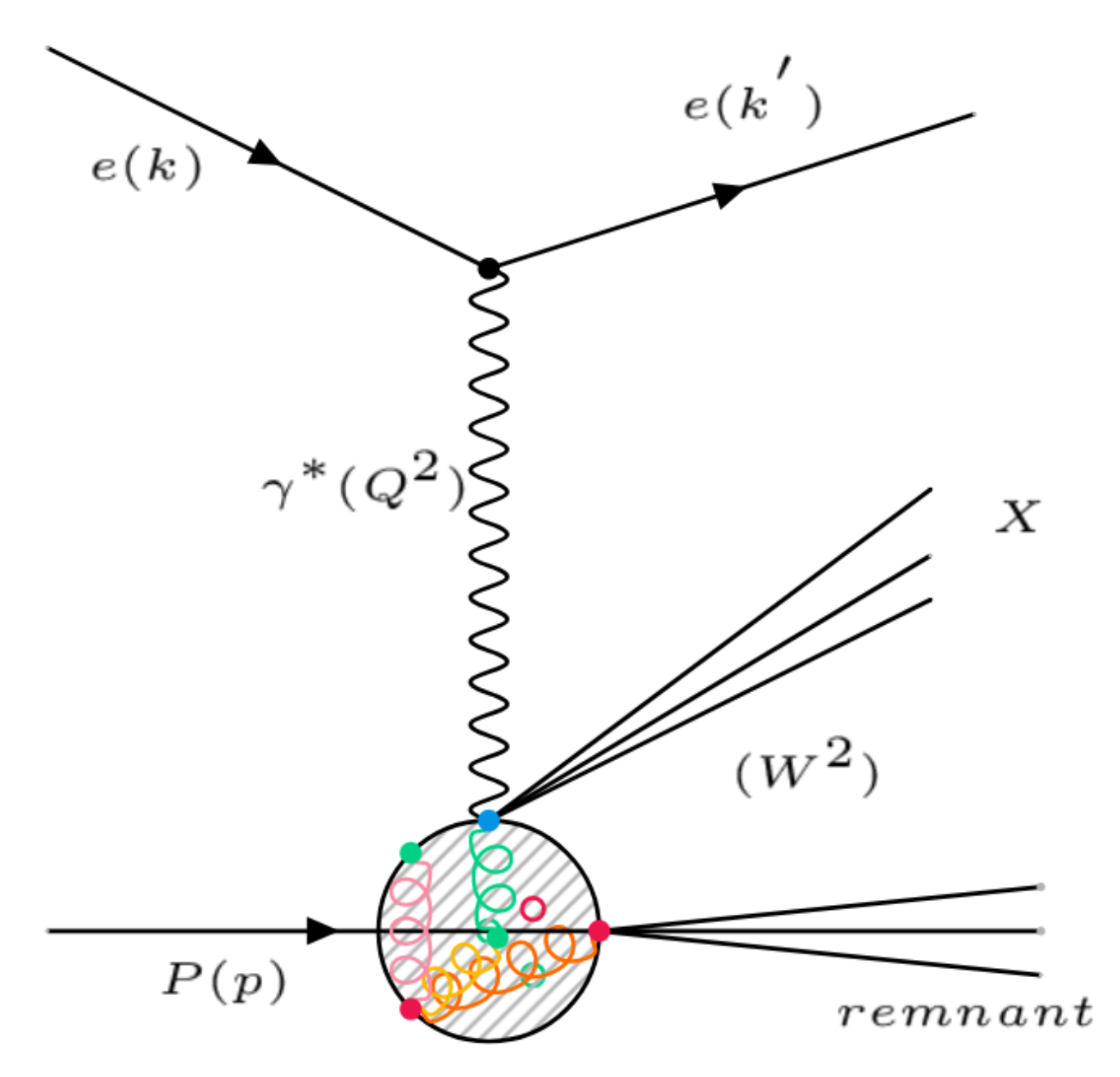
Figure 2.
Multiplicity distributions for shifted Gompertz distribution (SGD), Equation (11), fits to the data [33] in different ranges for 80 115 GeV. The lower panel shows the data/SGD-fit ratio plots for different regions.

Figure 3.
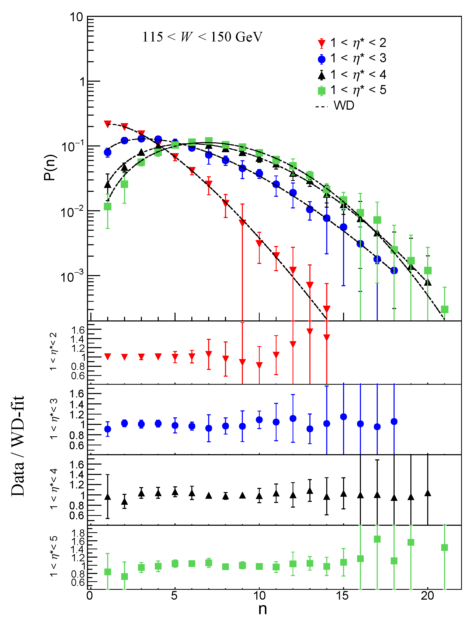
Multiplicity distributions for SGD fits to the data [33] in different ranges for 115 150 GeV. The lower panel shows the data/SGD-fit ratio plots for different regions.
Figure 3.
Multiplicity distributions for SGD fits to the data [33] in different ranges for 115 150 GeV. The lower panel shows the data/SGD-fit ratio plots for different regions.

Figure 4.
Multiplicity distributions for SGD fits to the data [33] in different ranges for 150 185 GeV. The lower panel shows the data/SGD-fit ratio plots for different regions.
Figure 4.
Multiplicity distributions for SGD fits to the data [33] in different ranges for 150 185 GeV. The lower panel shows the data/SGD-fit ratio plots for different regions.
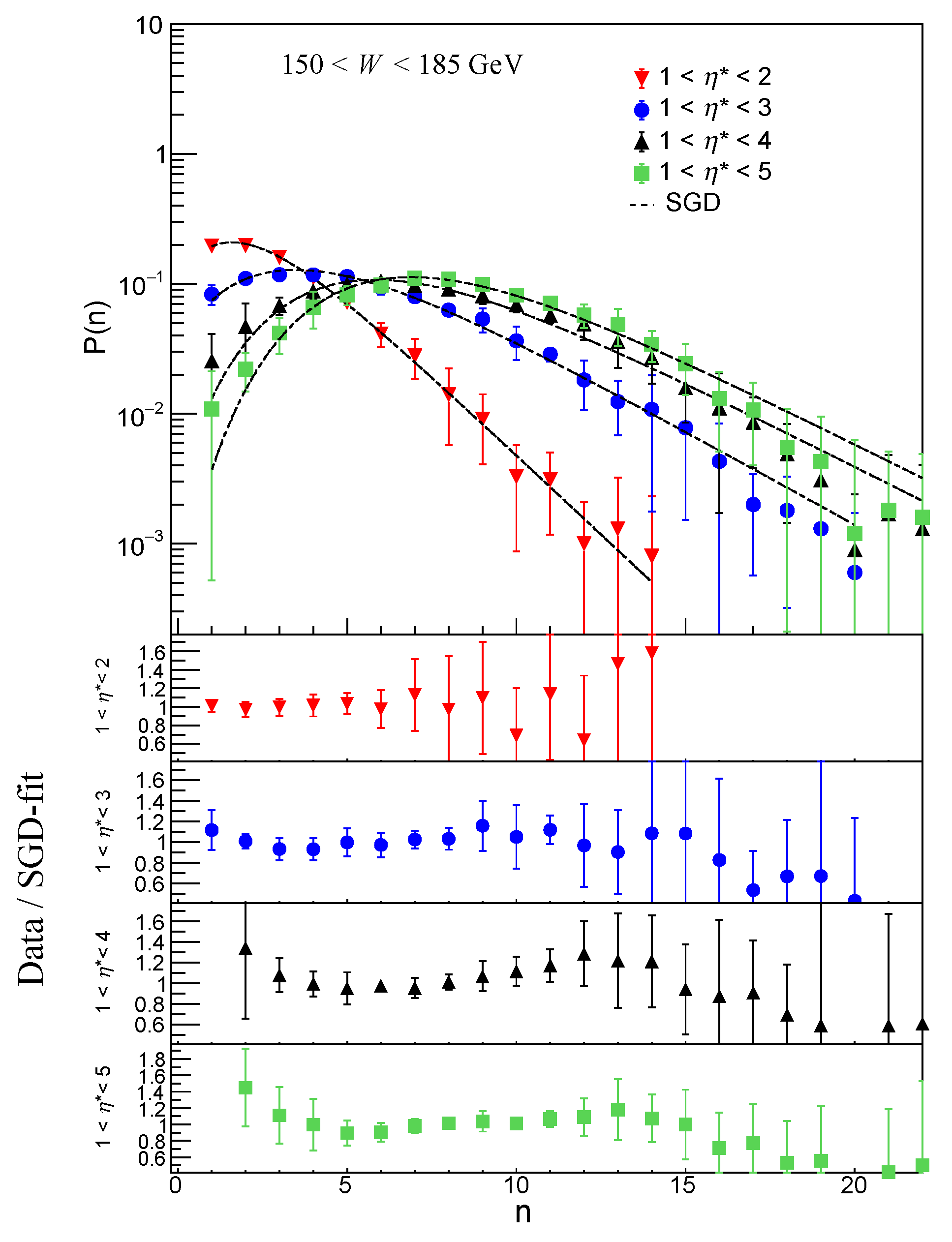
Figure 5.
Multiplicity distributions for SGD fits to the data [33] in different ranges for 185 (GeV) < 220. The lower panel shows the data/SGD-fit ratio plots for different regions.
Figure 5.
Multiplicity distributions for SGD fits to the data [33] in different ranges for 185 (GeV) < 220. The lower panel shows the data/SGD-fit ratio plots for different regions.
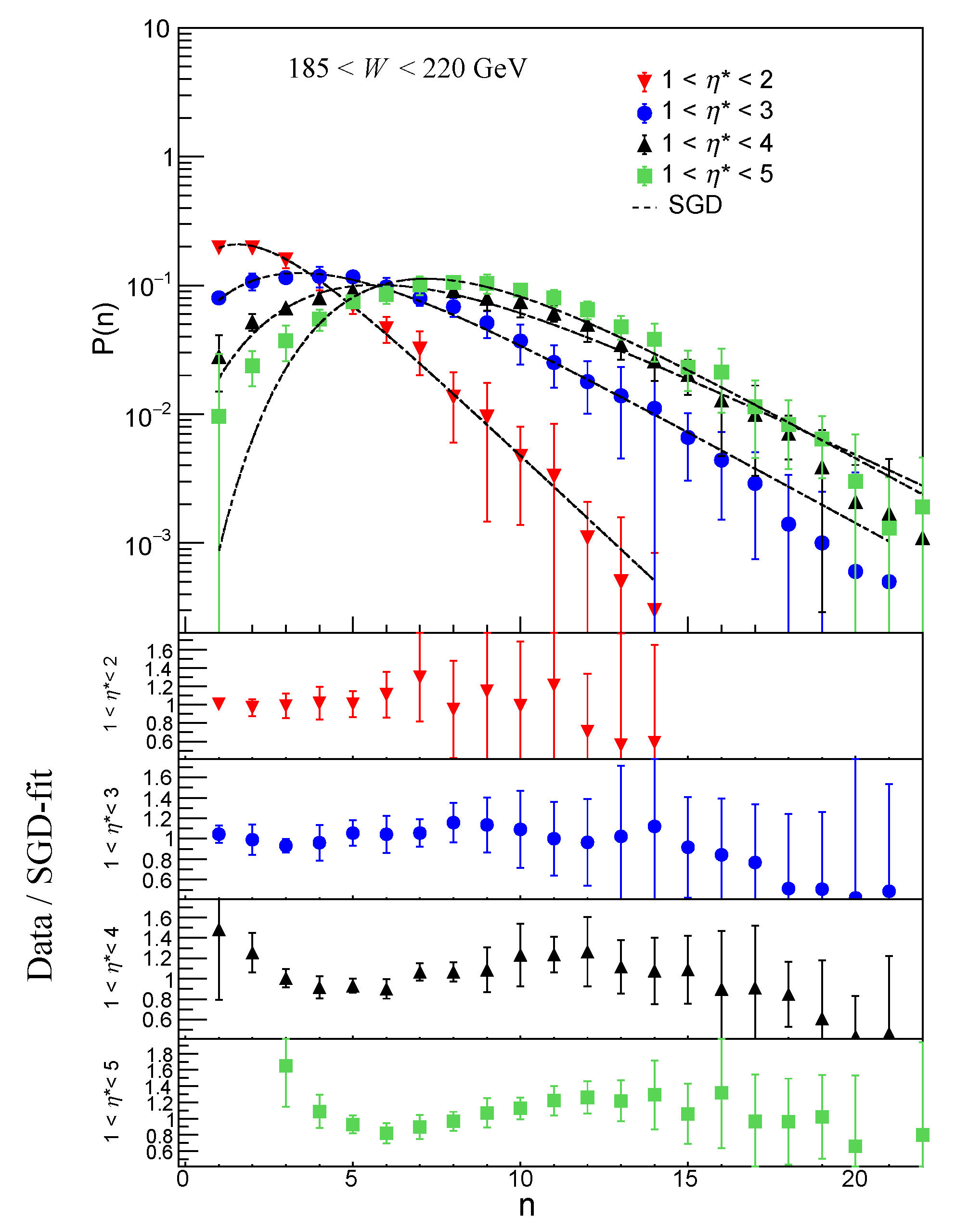
Figure 6.
Multiplicity distributions fits with Weibull (WD) probability function in 80 115 GeV in different ranges of the H1 data [33]. The lower panel shows the data/WD-fit ratio plots for different regions.
Figure 6.
Multiplicity distributions fits with Weibull (WD) probability function in 80 115 GeV in different ranges of the H1 data [33]. The lower panel shows the data/WD-fit ratio plots for different regions.
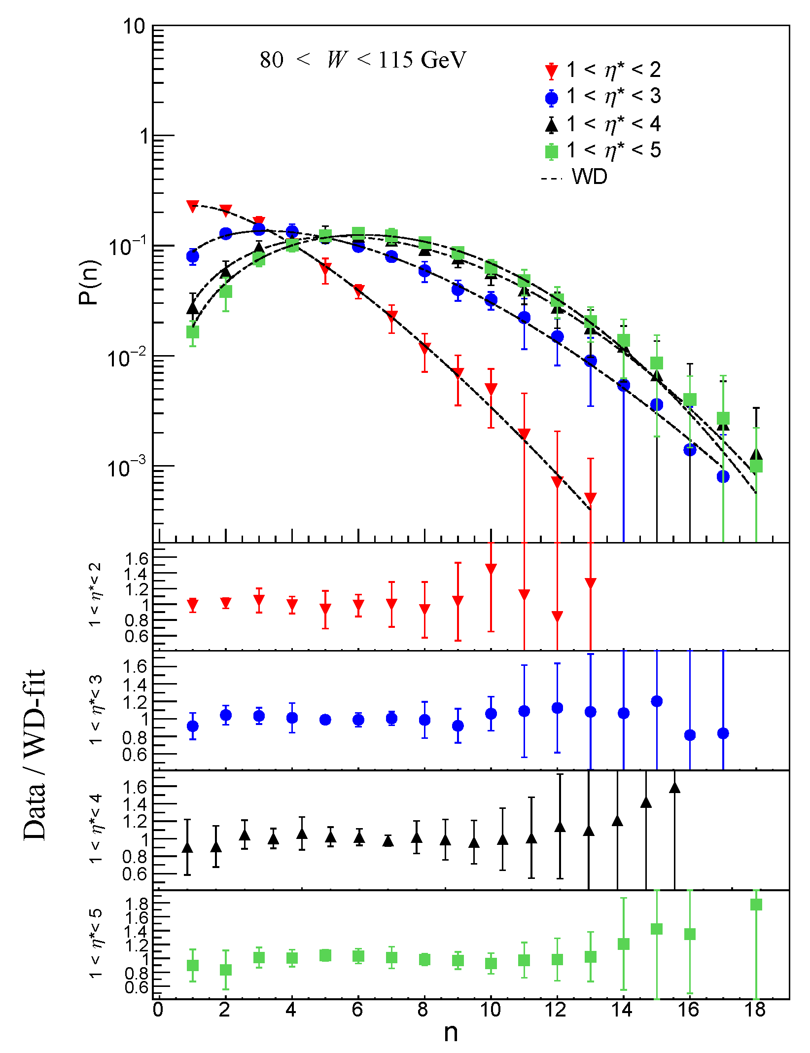
Figure 7.
Multiplicity distributions fits with the WD probability function in 115 150 GeV in different ranges of the H1 data [33]. The lower panel shows the data/WD-fit ratio plots for different regions.
Figure 7.
Multiplicity distributions fits with the WD probability function in 115 150 GeV in different ranges of the H1 data [33]. The lower panel shows the data/WD-fit ratio plots for different regions.

Figure 8.
Multiplicity distributions fits with the Weibull probability function in 150 185 GeV in different ranges of the H1 data [33]. The lower panel shows the data/WD-fit ratio plots for different regions.
Figure 8.
Multiplicity distributions fits with the Weibull probability function in 150 185 GeV in different ranges of the H1 data [33]. The lower panel shows the data/WD-fit ratio plots for different regions.
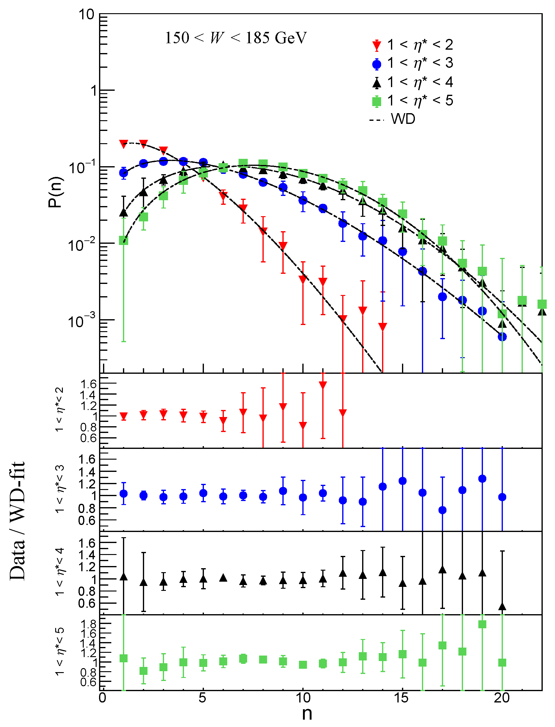
Figure 9.
Multiplicity distributions fits with the WD probability function in 185 220 GeV in different ranges of the H1 data [33]. The lower panel shows the data/WD-fit ratio plots for different regions.
Figure 9.
Multiplicity distributions fits with the WD probability function in 185 220 GeV in different ranges of the H1 data [33]. The lower panel shows the data/WD-fit ratio plots for different regions.
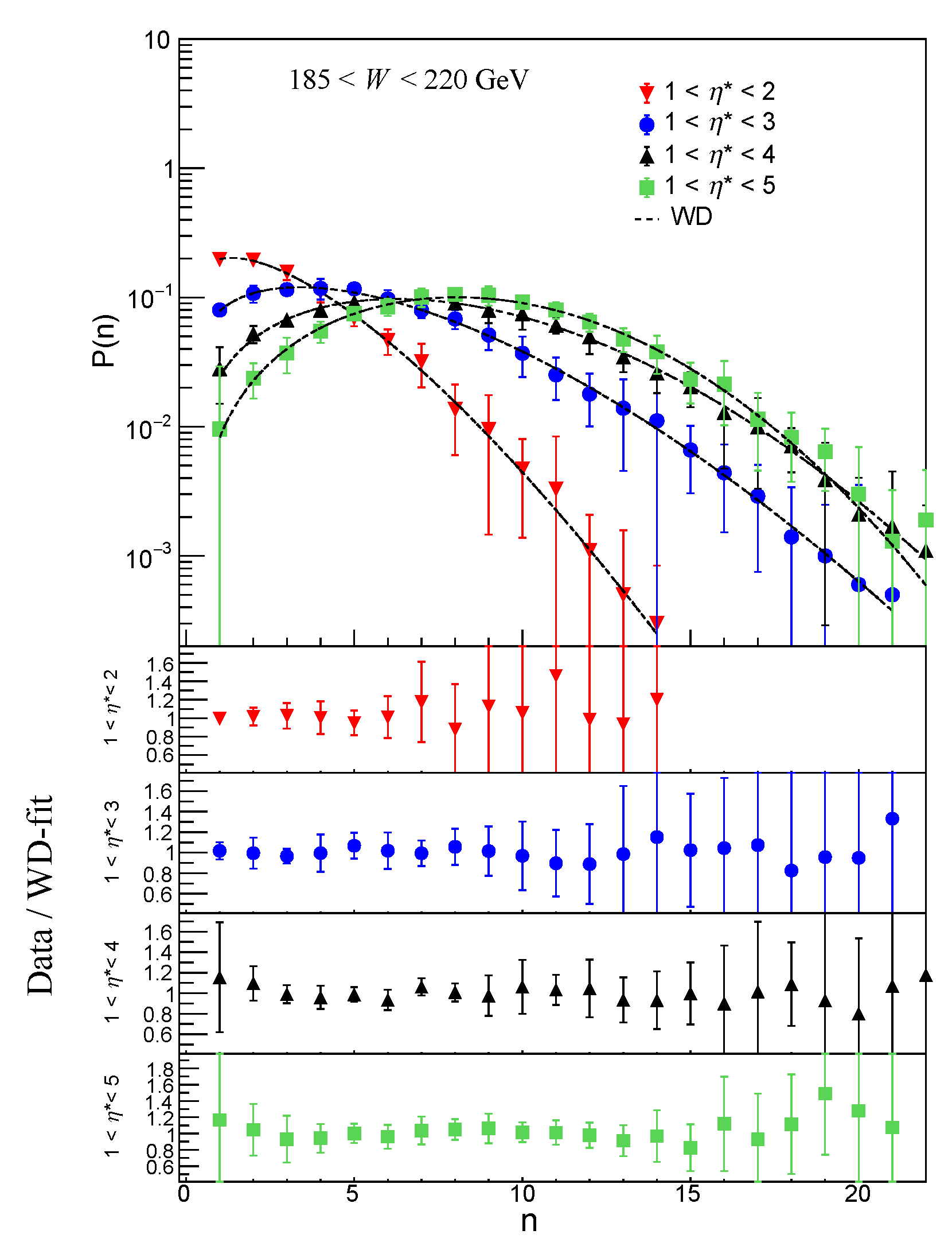
Figure 10.
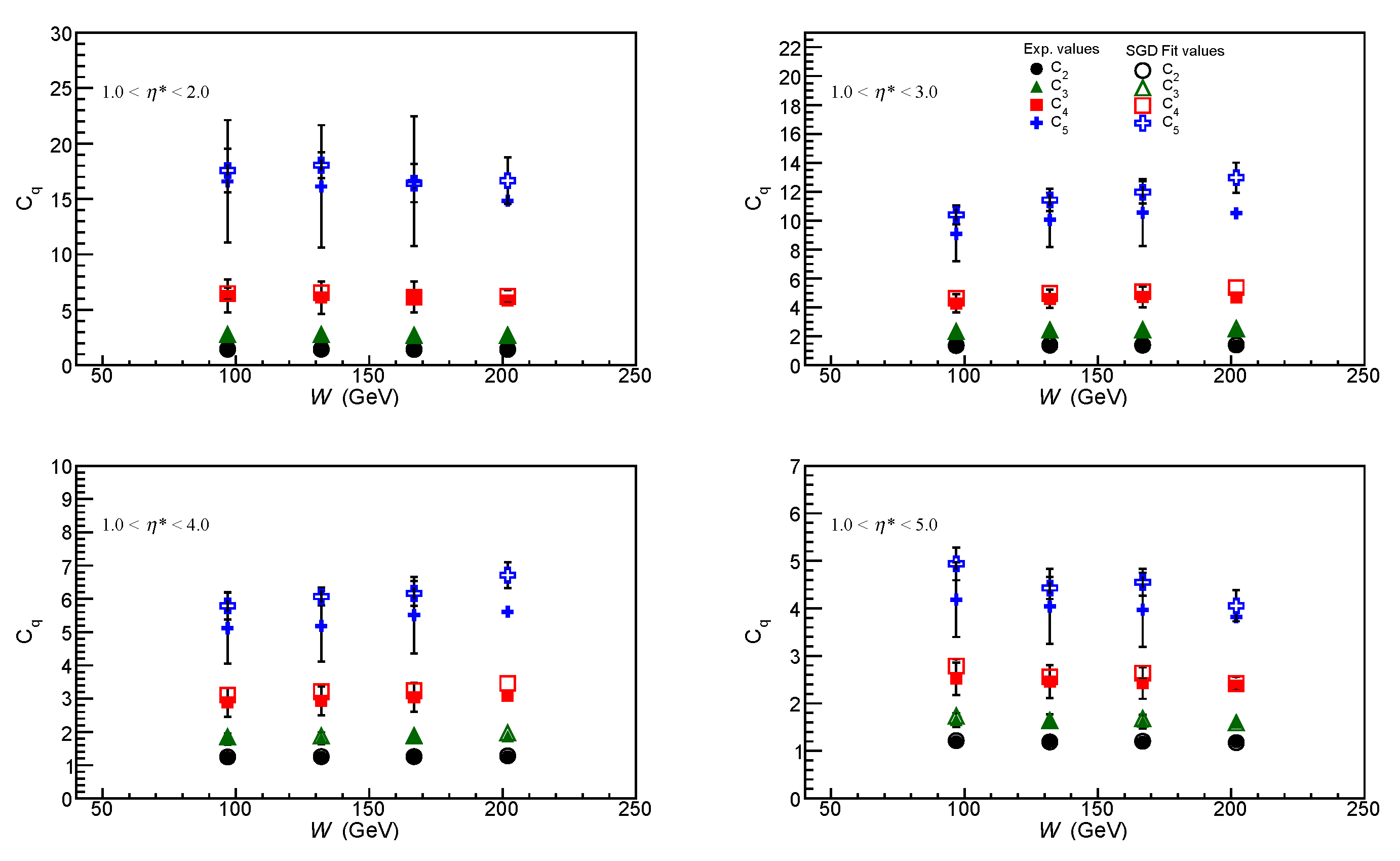
Normalized moments for q = 2, 3, 4, 5 for the SGD fits and comparison with the values calculated from the data [33] in different ranges.
Figure 10.
Normalized moments for q = 2, 3, 4, 5 for the SGD fits and comparison with the values calculated from the data [33] in different ranges.

Figure 11.
Normalized moments for q = 2, 3, 4, 5 for the WD fits and comparison with the values calculated from the data in different ranges of H1 data [33].
Figure 11.
Normalized moments for q = 2, 3, 4, 5 for the WD fits and comparison with the values calculated from the data in different ranges of H1 data [33].
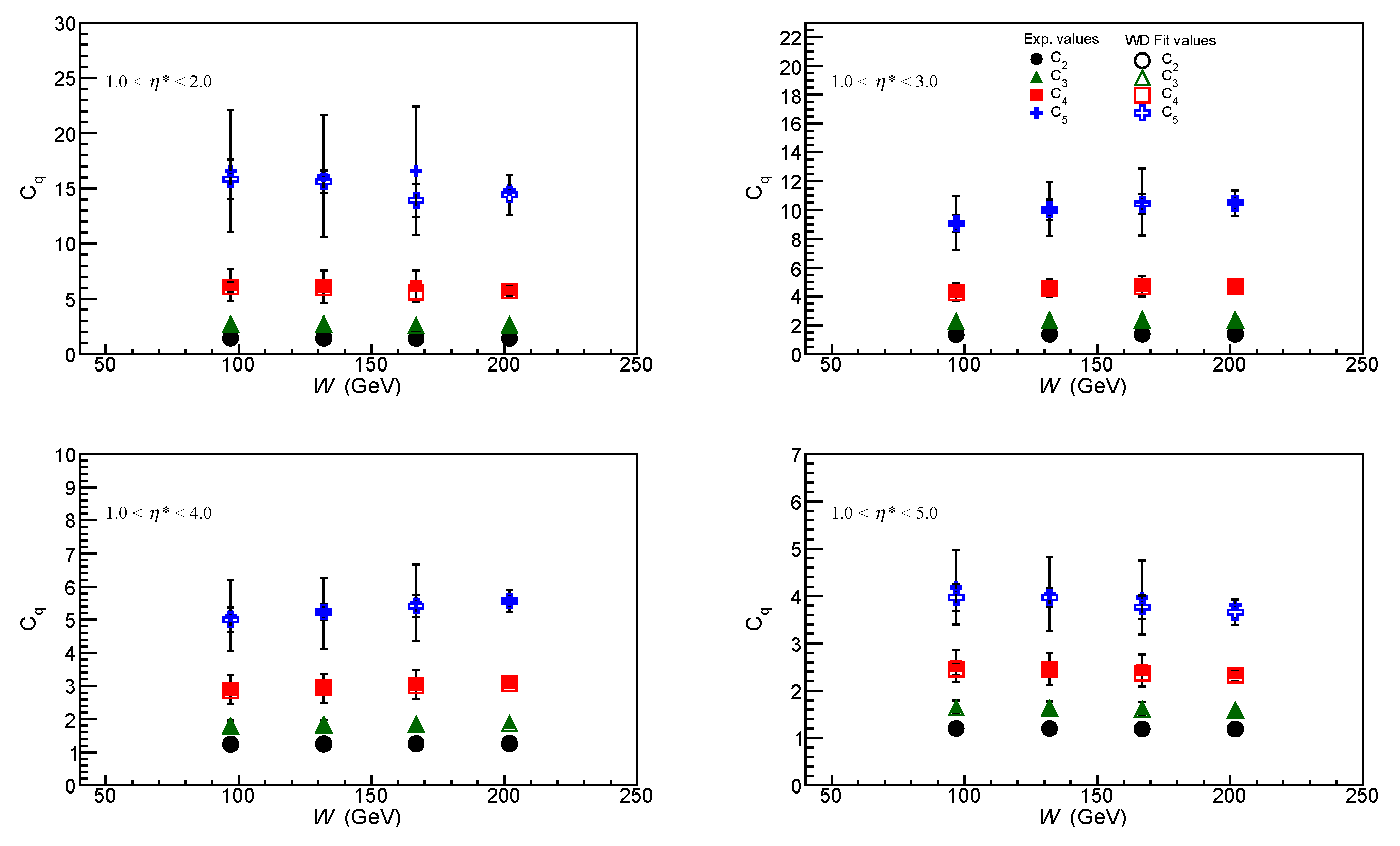
Figure 12.
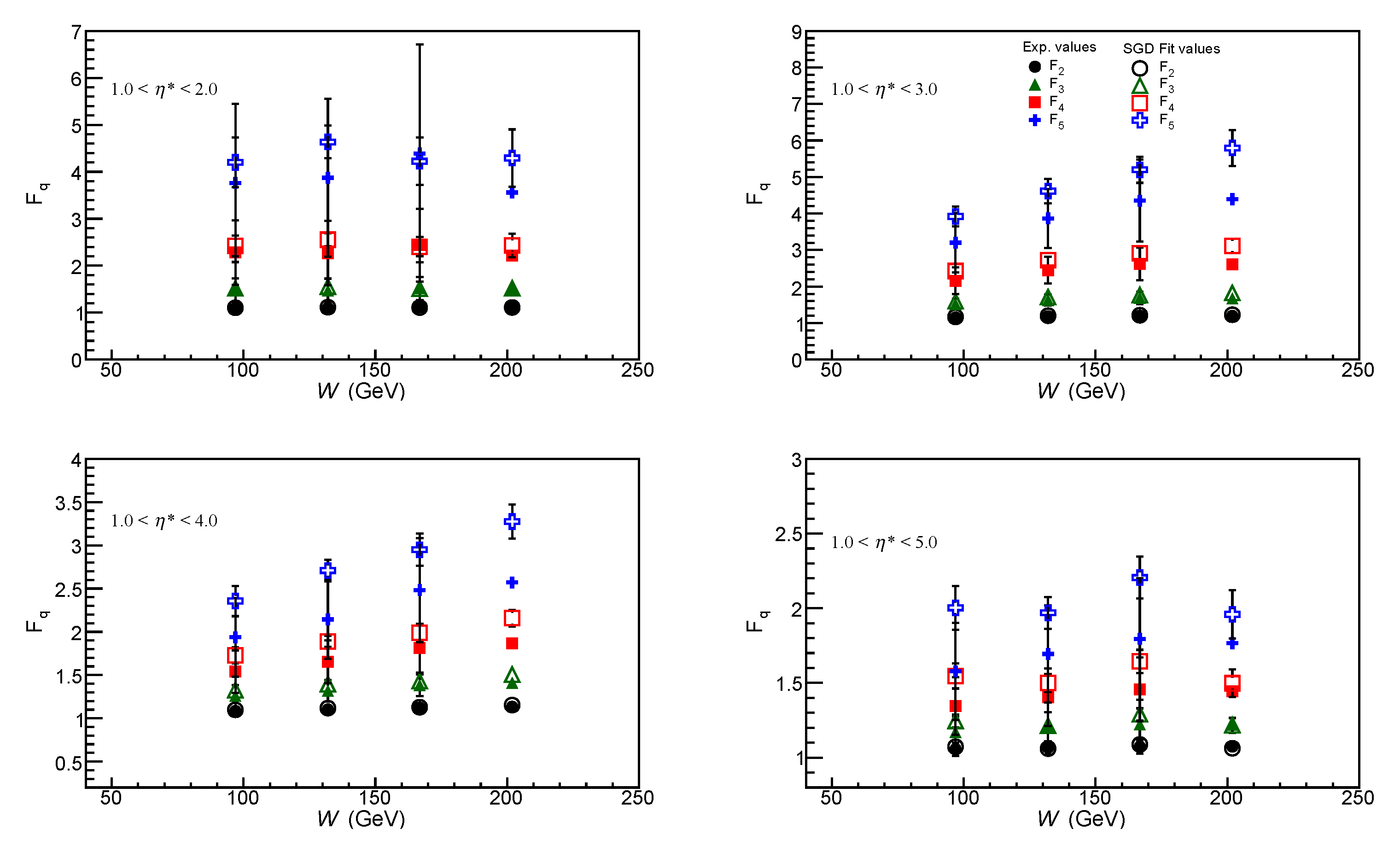
Normalized factorial moments for q = 2, 3, 4, 5 for the SGD fits and comparison with the values calculated from the data in different ranges of H1 data [33].
Figure 12.
Normalized factorial moments for q = 2, 3, 4, 5 for the SGD fits and comparison with the values calculated from the data in different ranges of H1 data [33].

Figure 13.
Normalized factorial moments for q = 2, 3, 4, 5 for the WD fits and comparison with the values calculated from the data [33] in different ranges.
Figure 13.
Normalized factorial moments for q = 2, 3, 4, 5 for the WD fits and comparison with the values calculated from the data [33] in different ranges.
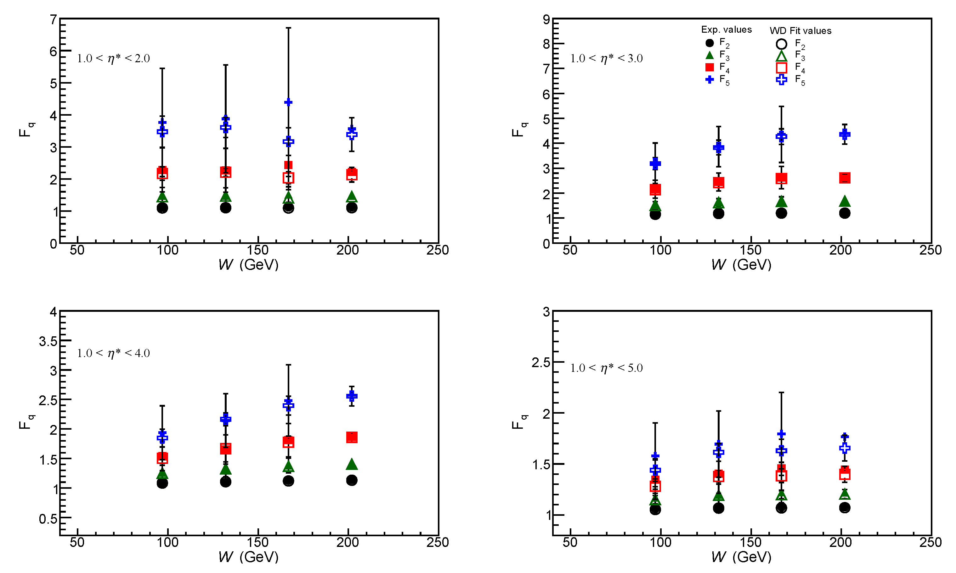
Figure 14.
moments from the SGD and WD fits in comparison to the data [33] for different W ranges and different intervals.
Figure 14.
moments from the SGD and WD fits in comparison to the data [33] for different W ranges and different intervals.
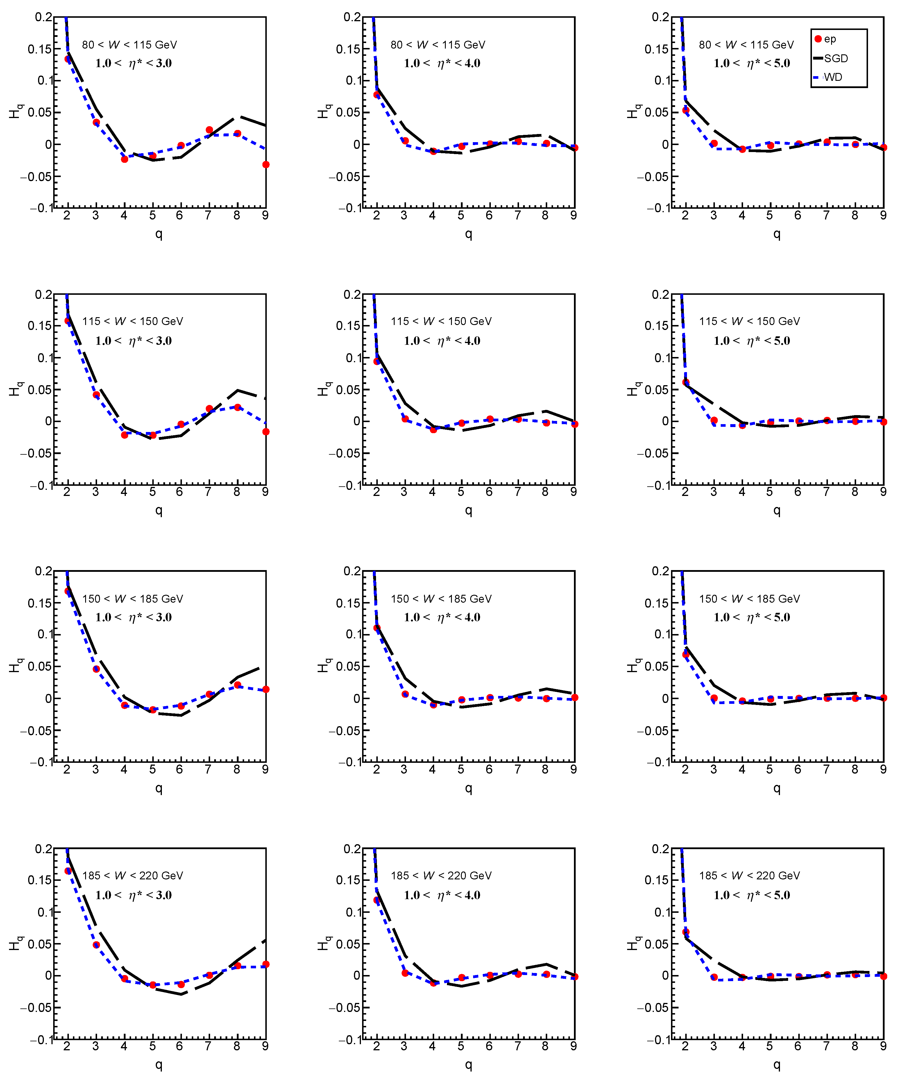
Figure 15.
Mean multiplicity versus dependence for ep collisions [33]. Experimental values are compared with the predicted values from the SGD and WD models. Shown also are the expected at the future proposed high energy ep colliders.
Figure 15.
Mean multiplicity versus dependence for ep collisions [33]. Experimental values are compared with the predicted values from the SGD and WD models. Shown also are the expected at the future proposed high energy ep colliders.
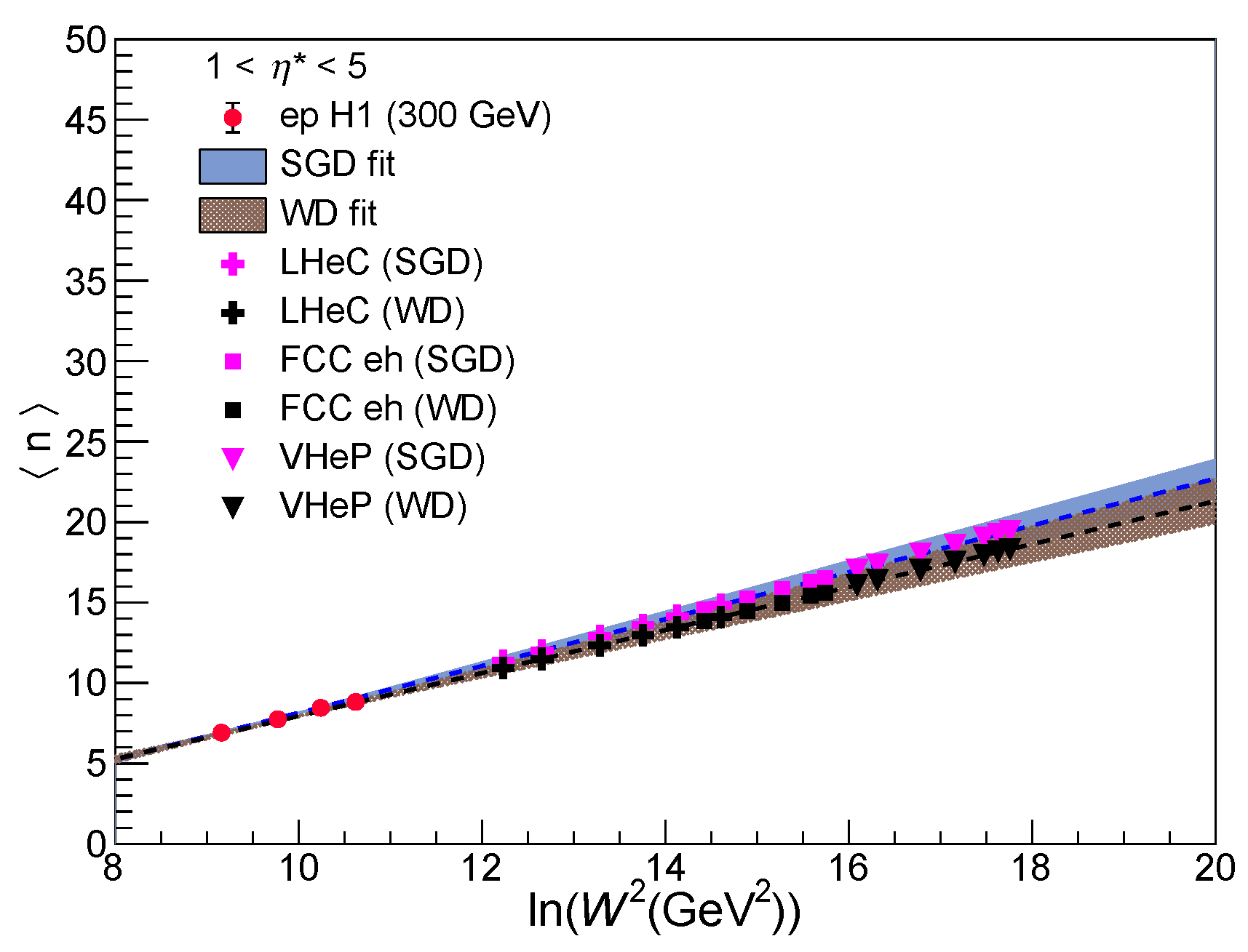
Figure 16.
for ee at LEP [53,54,55,56,57], p at SPS [41,58], pp at LHC [59,60] and ep at HERA [33] collisions versus /, compared with the predictions from SGD (dotted lines).


Table 1.
Shifted Gompertz distribution, Equation (10), fit parameters , the normalisation constant c, and /ndf (number of degrees of freedom) for the multiplicity distributions for 0 in different W ranges of the H1 data [33].
| c | b | t | ndf | |
|---|---|---|---|---|
| 80 115 GeV | ||||
| 1.0 2.0 | 0.92 ± 0.04 | 0.57 ± 0.03 | 1.31 ± 0.33 | 0.67/10 |
| 1.0 3.0 | 0.98 ± 0.04 | 0.38 ± 0.02 | 2.56 ± 0.30 | 4.26/14 |
| 1.0 4.0 | 1.00 ± 0.04 | 0.36 ± 0.02 | 5.03 ± 0.65 | 5.63/15 |
| 1.0 5.0 | 0.98 ± 0.04 | 0.37 ± 0.01 | 6.29 ± 0.69 | 15.23/15 |
| 115 150 GeV | ||||
| 1.0 2.0 | 0.90 ± 0.03 | 0.56 ± 0.02 | 1.37 ± 0.19 | 2.95/11 |
| 1.0 3.0 | 0.98 ± 0.03 | 0.34 ± 0.02 | 2.20 ± 0.26 | 3.09/15 |
| 1.0 4.0 | 0.98 ± 0.03 | 0.32 ± 0.01 | 4.81 ± 0.39 | 13.72/17 |
| 1.0 5.0 | 0.94 ± 0.03 | 0.36 ± 0.01 | 8.50 ± 0.79 | 35.25/18 |
| 150 185 GeV | ||||
| 1.0 2.0 | 0.90 ± 0.04 | 0.56 ± 0.03 | 1.62 ± 0.29 | 1.15/11 |
| 1.0 3.0 | 0.98 ± 0.03 | 0.33 ± 0.01 | 2.28 ± 0.28 | 5.17/17 |
| 1.0 4.0 | 0.95 ± 0.04 | 0.30 ± 0.01 | 4.89 ± 0.66 | 9.97/19 |
| 1.0 5.0 | 1.01 ± 0.04 | 0.30 ± 0.01 | 6.95 ± 0.95 | 7.42/19 |
| 185 220 GeV | ||||
| 1.0 2.0 | 0.90 ± 0.04 | 0.56 ± 0.03 | 1.58 ± 0.30 | 1.29/11 |
| 1.0 3.0 | 0.96 ± 0.04 | 0.33 ± 0.01 | 2.16 ± 0.22 | 4.23/18 |
| 1.0 4.0 | 0.95 ± 0.03 | 0.28 ± 0.01 | 4.05 ± 0.40 | 14.42/19 |
| 1.0 5.0 | 0.93 ± 0.04 | 0.33 ± 0.01 | 9.48 ± 1.34 | 24.74/20 |
Table 2.
Weibull distribution, Equation (A1), fit parameters with C as the normalisation constant for the multiplicity distributions for n > 0 in different W ranges of the H1 data [33].
| C | k | ndf | ||
|---|---|---|---|---|
| 80 115 GeV | ||||
| 1.0 2.0 | 0.92 ± 0.04 | 1.35 ± 0.08 | 2.93 ± 0.12 | 0.67 / 10 |
| 1.0 3.0 | 0.98 ± 0.04 | 1.67 ± 0.06 | 5.57 ± 0.16 | 1.08 / 14 |
| 1.0 4.0 | 0.98 ± 0.04 | 2.13 ± 0.09 | 7.27 ± 0.20 | 0.85 / 15 |
| 1.0 5.0 | 0.99 ± 0.04 | 2.38 ± 0.08 | 7.72 ± 0.17 | 1.97 / 15 |
| 115 150 GeV | ||||
| 1.0 2.0 | 0.90 ± 0.03 | 1.38 ± 0.04 | 3.05 ± 0.08 | 0.46/11 |
| 1.0 3.0 | 0.98 ± 0.03 | 1.61 ± 0.06 | 5.81 ± 0.16 | 1.40 /15 |
| 1.0 4.0 | 0.98 ± 0.03 | 2.09 ± 0.06 | 7.97 ± 0.15 | 2.01/17 |
| 1.0 5.0 | 1.00 ± 0.03 | 2.39 ± 0.08 | 8.59 ± 0.14 | 3.18/18 |
| 150 185 GeV | ||||
| 1.0 2.0 | 0.89 ± 0.03 | 1.44 ± 0.07 | 3.22 ± 0.10 | 1.26/11 |
| 1.0 3.0 | 0.97 ± 0.03 | 1.61 ± 0.06 | 6.10 ± 0.15 | 0.86/17 |
| 1.0 4.0 | 0.99 ± 0.04 | 2.06 ± 0.09 | 8.46 ± 0.21 | 1.37/19 |
| 1.0 5.0 | 0.98 ± 0.04 | 2.45 ± 0.11 | 9.33 ± 0.23 | 3.60/19 |
| 185 220 GeV | ||||
| 1.0 2.0 | 0.89 ± 0.04 | 1.42 ± 0.07 | 3.24 ± 0.12 | 0.53/11 |
| 1.0 3.0 | 0.97 ± 0.04 | 1.62 ± 0.05 | 6.15 ± 0.18 | 0.95/18 |
| 1.0 4.0 | 0.97 ± 0.03 | 2.02 ± 0.07 | 8.77 ± 0.19 | 2.03/19 |
| 1.0 5.0 | 0.99 ± 0.04 | 2.48 ± 0.11 | 9.92 ± 0.21 | 2.00/20 |
Table 3.
Normalised moments and normalised factorial moments calculated from the SGD fits to the data [33] for different W ranges.
Table 3.
Normalised moments and normalised factorial moments calculated from the SGD fits to the data [33] for different W ranges.
| 80 115 GeV | ||||||||
| 1.0 2.0 | 1.446 ± 0.040 | 2.76 ± 0.15 | 6.47 ± 0.54 | 17.57 ± 1.96 | 1.104 ± 0.033 | 1.51 ± 0.09 | 2.42 ± 0.22 | 4.20 ± 0.53 |
| 1.0 3.0 | 1.366 ± 0.021 | 2.33 ± 0.07 | 4.64 ± 0.22 | 10.40 ± 0.66 | 1.169 ± 0.018 | 1.59 ± 0.05 | 2.42 ± 0.12 | 3.92 ± 0.27 |
| 1.0 4.0 | 1.249 ± 0.022 | 1.85 ± 0.07 | 3.11 ± 0.16 | 5.79 ± 0.41 | 1.097 ± 0.020 | 1.33 ± 0.05 | 1.73 ± 0.09 | 2.36 ± 0.18 |
| 1.0 5.0 | 1.217 ± 0.021 | 1.73 ± 0.06 | 2.79 ± 0.15 | 4.94 ± 0.35 | 1.073 ± 0.019 | 1.25 ± 0.04 | 1.55 ± 0.08 | 2.00 ± 0.15 |
| 115 150 GeV | ||||||||
| 1.0 2.0 | 1.448 ± 0.022 | 2.78 ± 0.08 | 6.55 ± 0.31 | 18.05 ± 1.16 | 1.115 ± 0.018 | 1.55 ± 0.05 | 2.55 ± 0.14 | 4.63 ± 0.35 |
| 1.0 3.0 | 1.391 ± 0.022 | 2.43 ± 0.08 | 4.97 ± 0.25 | 11.43 ± 0.77 | 1.202 ± 0.019 | 1.71 ± 0.06 | 2.72 ± 0.14 | 4.61 ± 0.33 |
| 1.0 4.0 | 1.257 ± 0.014 | 1.88 ± 0.04 | 3.21 ± 0.10 | 6.07 ± 0.27 | 1.118 ± 0.012 | 1.39 ± 0.03 | 1.89 ± 0.06 | 2.71 ± 0.12 |
| 1.0 5.0 | 1.189 ± 0.016 | 1.64 ± 0.04 | 2.56 ± 0.10 | 4.43 ± 0.23 | 1.060 ± 0.014 | 1.21 ± 0.03 | 1.50 ± 0.06 | 1.97 ± 0.11 |
| 150 185 GeV | ||||||||
| 1.0 2.0 | 1.430 ± 0.035 | 2.68 ± 0.13 | 6.15 ± 0.47 | 16.43 ± 1.72 | 1.108 ± 0.029 | 1.51 ± 0.08 | 2.40 ± 0.21 | 4.22 ± 0.51 |
| 1.0 3.0 | 1.394 ± 0.022 | 2.45 ± 0.08 | 5.09 ± 0.25 | 11.97 ± 0.78 | 1.214 ± 0.020 | 1.76 ± 0.06 | 2.91 ± 0.15 | 5.20 ± 0.36 |
| 1.0 4.0 | 1.258 ± 0.019 | 1.89 ± 0.06 | 3.24 ± 0.14 | 6.17 ± 0.37 | 1.128 ± 0.017 | 1.43 ± 0.04 | 1.99 ± 0.09 | 2.95 ± 0.19 |
| 1.0 5.0 | 1.203 ± 0.019 | 1.68 ± 0.05 | 2.64 ± 0.12 | 4.55 ± 0.28 | 1.088 ± 0.017 | 1.29 ± 0.04 | 1.64 ± 0.08 | 2.20 ± 0.14 |
| 185 220 GeV | ||||||||
| 1.0 2.0 | 1.433 ± 0.042 | 2.70 ± 0.16 | 6.21 ± 0.58 | 16.66 ± 2.10 | 1.110 ± 0.034 | 1.52 ± 0.10 | 2.43 ± 0.25 | 4.29 ± 0.61 |
| 1.0 3.0 | 1.408 ± 0.026 | 2.52 ± 0.10 | 5.36 ± 0.32 | 12.98 ± 1.04 | 1.228 ± 0.023 | 1.82 ± 0.07 | 3.11 ± 0.19 | 5.80 ± 0.49 |
| 1.0 4.0 | 1.282 ± 0.018 | 1.97 ± 0.06 | 3.46 ± 0.15 | 6.71 ± 0.39 | 1.153 ± 0.016 | 1.51 ± 0.04 | 2.16 ± 0.10 | 3.27 ± 0.20 |
| 1.0 5.0 | 1.175 ± 0.023 | 1.59 ± 0.06 | 2.41 ± 0.15 | 4.05 ± 0.33 | 1.062 ± 0.021 | 1.22 ± 0.05 | 1.50 ± 0.09 | 1.96 ± 0.16 |
Table 4.
Normalised moments and normalised factorial moments calculated from the WD fits to the data [33] for different W ranges.
Table 4.
Normalised moments and normalised factorial moments calculated from the WD fits to the data [33] for different W ranges.
| 80 115 GeV | ||||||||
| 1.0 2.0 | 1.437 ± 0.038 | 2.69 ± 0.15 | 6.08 ± 0.51 | 15.83 ± 1.80 | 1.094 ± 0.031 | 1.45 ± 0.09 | 2.17 ± 0.21 | 3.47 ± 0.49 |
| 1.0 3.0 | 1.352 ± 0.020 | 2.23 ± 0.07 | 4.27 ± 0.20 | 9.07 ± 0.60 | 1.153 ± 0.018 | 1.51 ± 0.05 | 2.14 ± 0.11 | 3.18 ± 0.24 |
| 1.0 4.0 | 1.240 ± 0.022 | 1.78 ± 0.06 | 2.86 ± 0.16 | 5.00 ± 0.37 | 1.085 ± 0.019 | 1.25 ± 0.05 | 1.51 ± 0.09 | 1.85 ± 0.15 |
| 1.0 5.0 | 1.199 ± 0.020 | 1.63 ± 0.06 | 2.45 ± 0.13 | 3.97 ± 0.29 | 1.053 ± 0.018 | 1.15 ± 0.04 | 1.28 ± 0.07 | 1.44 ± 0.11 |
| 115 150 GeV | ||||||||
| 1.0 2.0 | 1.434 ± 0.021 | 2.67 ± 0.08 | 6.01 ± 0.28 | 15.61 ± 1.04 | 1.101 ± 0.017 | 1.46 ± 0.05 | 2.20 ± 0.13 | 3.60 ± 0.31 |
| 1.0 3.0 | 1.375 ± 0.021 | 2.33 ± 0.07 | 4.57 ± 0.23 | 10.02 ± 0.70 | 1.185 ± 0.019 | 1.62 ± 0.05 | 2.42 ± 0.13 | 3.83 ± 0.29 |
| 1.0 4.0 | 1.248 ± 0.013 | 1.81 ± 0.04 | 2.95 ± 0.10 | 5.23 ± 0.24 | 1.107 ± 0.012 | 1.32 ± 0.03 | 1.67 ± 0.06 | 2.16 ± 0.11 |
| 1.0 5.0 | 1.198 ± 0.015 | 1.63 ± 0.04 | 2.45 ± 0.09 | 3.97 ± 0.20 | 1.067 ± 0.013 | 1.19 ± 0.03 | 1.38 ± 0.05 | 1.61 ± 0.09 |
| 150 185 GeV | ||||||||
| 1.0 2.0 | 1.414 ± 0.033 | 2.56 ± 0.13 | 5.58 ± 0.43 | 13.91 ± 1.49 | 1.092 ± 0.027 | 1.41 ± 0.08 | 2.03 ± 0.19 | 3.16 ± 0.43 |
| 1.0 3.0 | 1.380 ± 0.021 | 2.36 ± 0.07 | 4.68 ± 0.22 | 10.42 ± 0.69 | 1.199 ± 0.019 | 1.67 ± 0.05 | 2.59 ± 0.13 | 4.27 ± 0.31 |
| 1.0 4.0 | 1.254 ± 0.018 | 1.83 ± 0.05 | 3.01 ± 0.13 | 5.41 ± 0.34 | 1.121 ± 0.016 | 1.37 ± 0.04 | 1.78 ± 0.08 | 2.40 ± 0.16 |
| 1.0 5.0 | 1.190 ± 0.019 | 1.60 ± 0.05 | 2.36 ± 0.11 | 3.77 ± 0.25 | 1.069 ± 0.017 | 1.20 ± 0.04 | 1.38 ± 0.07 | 1.63 ± 0.11 |
| 185 220 GeV | ||||||||
| 1.0 2.0 | 1.422 ± 0.039 | 2.60 ± 0.15 | 5.72 ± 0.52 | 14.41 ± 1.82 | 1.102 ± 0.032 | 1.44 ± 0.09 | 2.13 ± 0.23 | 3.38 ± 0.52 |
| 1.0 3.0 | 1.379 ± 0.025 | 2.35 ± 0.09 | 4.69 ± 0.28 | 10.48 ± 0.87 | 1.200 ± 0.022 | 1.68 ± 0.07 | 2.61 ± 0.17 | 4.36 ± 0.40 |
| 1.0 4.0 | 1.261 ± 0.018 | 1.86 ± 0.05 | 3.08 ± 0.14 | 5.57 ± 0.34 | 1.132 ± 0.016 | 1.41 ± 0.04 | 1.86 ± 0.09 | 2.56 ± 0.16 |
| 1.0 5.0 | 1.185 ± 0.021 | 1.58 ± 0.06 | 2.32 ± 0.13 | 3.66 ± 0.27 | 1.071 ± 0.019 | 1.20 ± 0.04 | 1.40 ± 0.08 | 1.66 ± 0.13 |
Table 5.
Normalised moments and normalised factorial moments calculated from the data [33] for different W ranges.
Table 5.
Normalised moments and normalised factorial moments calculated from the data [33] for different W ranges.
| 80 115 GeV | ||||||||
| 1.0 2.0 | 1.440 ± 0.095 | 2.72 ± 0.39 | 6.26 ± 1.47 | 16.59 ± 5.53 | 1.098 ± 0.078 | 1.48 ± 0.25 | 2.28 ± 0.68 | 3.76 ± 1.68 |
| 1.0 3.0 | 1.353 ± 0.059 | 2.24 ± 0.20 | 4.28 ± 0.62 | 9.09 ± 1.88 | 1.155 ± 0.051 | 1.52 ± 0.15 | 2.16 ± 0.36 | 3.20 ± 0.81 |
| 1.0 4.0 | 1.239 ± 0.058 | 1.79 ± 0.17 | 2.89 ± 0.43 | 5.12 ± 1.07 | 1.084 ± 0.051 | 1.26 ± 0.12 | 1.54 ± 0.25 | 1.94 ± 0.46 |
| 1.0 5.0 | 1.201 ± 0.052 | 1.65 ± 0.15 | 2.52 ± 0.34 | 4.18 ± 0.79 | 1.056 ± 0.045 | 1.17 ± 0.10 | 1.35 ± 0.19 | 1.58 ± 0.32 |
| 115 150 GeV | ||||||||
| 1.0 2.0 | 1.435 ± 0.050 | 2.68 ± 0.22 | 6.10 ± 0.89 | 16.13 ± 3.65 | 1.101 ± 0.042 | 1.47 ± 0.16 | 2.27 ± 0.47 | 3.87 ± 1.34 |
| 1.0 3.0 | 1.376 ± 0.072 | 2.34 ± 0.26 | 4.60 ± 0.83 | 10.06 ± 2.54 | 1.187 ± 0.062 | 1.63 ± 0.19 | 2.45 ± 0.48 | 3.86 ± 1.10 |
| 1.0 4.0 | 1.245 ± 0.040 | 1.80 ± 0.12 | 2.93 ± 0.31 | 5.19 ± 0.76 | 1.104 ± 0.036 | 1.32 ± 0.09 | 1.65 ± 0.18 | 2.14 ± 0.35 |
| 1.0 5.0 | 1.195 ± 0.039 | 1.63 ± 0.11 | 2.46 ± 0.26 | 4.04 ± 0.59 | 1.065 ± 0.035 | 1.20 ± 0.08 | 1.40 ± 0.15 | 1.69 ± 0.28 |
| 150 185 GeV | ||||||||
| 1.0 2.0 | 1.431 ± 0.079 | 2.68 ± 0.34 | 6.17 ± 1.41 | 16.61 ± 5.85 | 1.111 ± 0.067 | 1.51 ± 0.24 | 2.44 ± 0.78 | 4.39 ± 2.32 |
| 1.0 3.0 | 1.383 ± 0.062 | 2.37 ± 0.23 | 4.72 ± 0.72 | 10.56 ± 2.32 | 1.203 ± 0.054 | 1.69 ± 0.17 | 2.62 ± 0.45 | 4.35 ± 1.12 |
| 1.0 4.0 | 1.256 ± 0.054 | 1.84 ± 0.16 | 3.04 ± 0.44 | 5.51 ± 1.15 | 1.124 ± 0.048 | 1.38 ± 0.13 | 1.81 ± 0.28 | 2.48 ± 0.60 |
| 1.0 5.0 | 1.192 ± 0.051 | 1.62 ± 0.14 | 2.43 ± 0.33 | 3.97 ± 0.78 | 1.074 ± 0.046 | 1.22 ± 0.11 | 1.46 ± 0.21 | 1.79 ± 0.41 |
| 185 220 GeV | ||||||||
| 1.0 2.0 | 1.427 ± 0.100 | 2.63 ± 0.41 | 5.84 ± 1.47 | 14.84 ± 5.35 | 1.110 ± 0.083 | 1.48 ± 0.27 | 2.22 ± 0.71 | 3.56 ± 1.72 |
| 1.0 3.0 | 1.376 ± 0.078 | 2.35 ± 0.29 | 4.68 ± 0.95 | 10.52 ± 3.13 | 1.197 ± 0.069 | 1.67 ± 0.22 | 2.61 ± 0.59 | 4.39 ± 1.57 |
| 1.0 4.0 | 1.264 ± 0.058 | 1.87 ± 0.18 | 3.09 ± 0.47 | 5.61 ± 1.19 | 1.135 ± 0.052 | 1.41 ± 0.14 | 1.86 ± 0.30 | 2.57 ± 0.59 |
| 1.0 5.0 | 1.187 ± 0.057 | 1.60 ± 0.16 | 2.37 ± 0.36 | 3.82 ± 0.79 | 1.074 ± 0.051 | 1.22 ± 0.12 | 1.44 ± 0.22 | 1.77 ± 0.38 |
Table 6.
Comparison of experimental average multiplicity with the corresponding values obtained from SGD and WD fits to the data [33] at various W and intervals.
Table 6.
Comparison of experimental average multiplicity with the corresponding values obtained from SGD and WD fits to the data [33] at various W and intervals.
| Exp. Value | SGD Fit | WD Fit | ||
|---|---|---|---|---|
| (GeV) | ||||
| 80 115 | 1.0 2.0 | 2.92 ± 0.17 | 2.93 ± 0.07 | 2.91 ± 0.07 |
| 1.0 3.0 | 5.06 ± 0.28 | 5.06 ± 0.08 | 5.03 ± 0.09 | |
| 1.0 4.0 | 6.49 ± 0.37 | 6.61 ± 0.11 | 6.44 ± 0.13 | |
| 1.0 5.0 | 6.91 ± 0.36 | 6.92 ± 0.11 | 6.85 ± 0.14 | |
| 115 150 | 1.0 2.0 | 3.00 ± 0.14 | 3.01 ± 0.04 | 3.00 ± 0.05 |
| 1.0 3.0 | 5.30 ± 0.32 | 5.27 ± 0.09 | 5.27 ± 0.09 | |
| 1.0 4.0 | 7.08 ± 0.29 | 7.17 ± 0.08 | 7.07 ± 0.09 | |
| 1.0 5.0 | 7.75 ± 0.35 | 7.78 ± 0.09 | 7.62 ± 0.11 | |
| 150 185 | 1.0 2.0 | 3.13 ± 0.18 | 3.11 ± 0.07 | 3.11 ± 0.08 |
| 1.0 3.0 | 5.54 ± 0.31 | 5.56 ± 0.08 | 5.53 ± 0.09 | |
| 1.0 4.0 | 7.58 ± 0.44 | 7.71 ± 0.11 | 7.50 ± 0.13 | |
| 1.0 5.0 | 8.46 ± 0.47 | 8.69 ± 0.13 | 8.27 ± 0.16 | |
| 185 220 | 1.0 2.0 | 3.15 ± 0.23 | 3.10 ± 0.09 | 3.13 ± 0.09 |
| 1.0 3.0 | 5.57 ± 0.39 | 5.56 ± 0.10 | 5.58 ± 0.11 | |
| 1.0 4.0 | 7.73 ± 0.43 | 7.77 ± 0.11 | 7.77 ± 0.12 | |
| 1.0 5.0 | 8.82 ± 0.49 | 8.88 ± 0.16 | 8.80 ± 0.17 |
Table 7.
The energies of electron (Ee) and proton (Ep) beams and the center-of-mass energy () at HERA and at the future ep colliders.
Table 7.
The energies of electron (Ee) and proton (Ep) beams and the center-of-mass energy () at HERA and at the future ep colliders.
| HERA-I | LHeC | FCC-eh | VHep | |
|---|---|---|---|---|
| Ee (GeV) | 27.5 | 60–140 | 60 | 3000 |
| Ep (TeV) | 0.9 | 7 | 50 | 7 |
| (TeV) | 0.3 | 1.2–1.9 | 3.5 | 9 |
Publisher’s Note: MDPI stays neutral with regard to jurisdictional claims in published maps and institutional affiliations. |
© 2021 by the authors. Licensee MDPI, Basel, Switzerland. This article is an open access article distributed under the terms and conditions of the Creative Commons Attribution (CC BY) license (https://creativecommons.org/licenses/by/4.0/).
Share and Cite
MDPI and ACS Style
Aggarwal, R.; Kaur, M. Statistical Scrutiny of Particle Spectra in ep Collisions. Physics 2021, 3, 757-780. https://doi.org/10.3390/physics3030047
AMA Style
Aggarwal R, Kaur M. Statistical Scrutiny of Particle Spectra in ep Collisions. Physics. 2021; 3(3):757-780. https://doi.org/10.3390/physics3030047
Chicago/Turabian StyleAggarwal, Ritu, and Manjit Kaur. 2021. "Statistical Scrutiny of Particle Spectra in ep Collisions" Physics 3, no. 3: 757-780. https://doi.org/10.3390/physics3030047