A Local and Time Resolution of the COVID-19 Propagation—A Two-Dimensional Approach for Germany Including Diffusion Phenomena to Describe the Spatial Spread of the COVID-19 Pandemic

Abstract

The understanding of factors that affect the dissemination of a viral infection is fundamental to help combat it. For instance, during the COVID-19 pandemic that changed the lives of people all over the world, one observes regions with different incidences of cases. One can speculate that population density might be one of the variables that affect the incidence of cases. In populous areas, such as big cities or congested urban areas, higher COVID-19 incidences could be observed than in rural regions. It is natural to think that if population density is such an important factor, then a gradient or difference in population density might lead to a diffusion process that will proceed until equilibrium is reached. The aim of this paper consists of the inclusion of a diffusion concept into the COVID-19 modeling. With this concept, one covers a gradient-driven transfer of the infection next to epidemic growth models (SIR-type models). This is discussed for a certain period of the German situation based on the quite different incidence data for the different federal states of Germany. With this ansatz, some phenomena of the actual development of the pandemic are found to be confirmed. The model provides a possibility to investigate certain scenarios, such as border-crossings or local spreading events, and their influence on the COVID-19 propagation. The resulting information can be a basis for the decisions of politicians and medical persons in charge of managing a pandemic.

1. Introduction

The curves of infected, susceptible and recovered people, which can be found in every newspaper, describe the global pandemic behavior of the whole country, e.g., Italy, France or Germany. The mathematical modeling of COVID-19 with susceptible-infected-recovered (SIR) type models [1,2,3,4,5,6,7] leads to averaged results and does not take into account unequal population numbers or population densities.

However, it is known that these issues play an important role in the local pandemic evolution (see, e.g., [8]). Based on the local-dependent density of people and a diffusion model, the COVID-19 propagation is considered here to be resolved in a finer manner.

The structure of this paper is organized as follows. In Section 2, the diffusion concept is explained. The German database is analyzed and discussed in Section 3. The numerical solution method of the initial boundary value diffusion problem is described in Section 4, and the qualitative properties of the diffusion model simulation results are given results in Section 5. In Section 6, local transmission effects are modeled, joined onto the diffusion model, and then, applied to the German pandemic situation in April/May 2021. Section 7 concludes the studies with a summary of main results.

2. The Mathematical Diffusion Model

What is a good choice of quantity to describe the COVID-19 spread? The World Health Organization (WHO) and national health institutions measure the COVID-19 spread with the seven-day incidence (WHO also uses the fourteen-days incidence) of people with COVID-19 per 100,000 inhabitants. In Germany, it is possible to control or trace the history of people with COVID-19 by local health institutions if the seven-day incidence has a value less than 50. However, between the end of December 2020 and the beginning of January 2021, the averaged incidence was about 140 and, in some hot-spot federal states, such as Saxony, it was greater than 300. At the end of March and at the beginning of April, the incidences changed dramatically. However, in general, one considers a different pandemic development from one federal state to another and this situation needs to be respected with the consideration of diffusion phenomena.

If the social and economical life should be sustained, there are several possibilities of transmitting the COVID-19 virus. Among others, the following ones to be mentioned:

• commuters and employers on the way to their office or to their position of employment, especially medical and nursing staff;
• pupils and teachers in schools and on the way to school;
• people buying everyday necessities using shopping centers;
• postmen, suppliers and deliverers.

All of these activities take place during so-called lock-downs in Germany, with the result of an ongoing propagation of the pandemic. Furthermore, the unavailable center of power in the decentralized federal states of Germany often leads to solo efforts of some federal states.

From authoritarian countries, such as China or Singapore, with quite a different civilization and cultural traditions than those in Germany, it is known that the virus propagation could be stopped with very rigorous measures such as the strict prohibition of social and economic life. Those ones mentioned-above are absolutely forbidden.

This is inconceivable in countries like Germany, Austria, the Netherlands or other so-called democratic states with a western understanding of freedom and self-determination. However, as a consequence of such a western lifestyle, they have to live with more or less consecutive activity of the COVID-19 pandemic. This is the reason for the following trial: to describe one aspect of the pandemic by a diffusion model. In connection with the pandemic, diffusion has been discussed, e.g., in [9,10,11]. The diffusion being a central process in many biological, social, chemical and physical systems is considered in [12,13]. A similar model but in another context has been discussed in [14].

Within the diffusion concept considered here, the seven-day incidence, denoted by s, serves as the quantity that is influenced by its gradients between different levels of incidence in the federal states of Germany. The mathematical model of diffusion of a certain quantity c is given by [15]:

$$\frac{\partial c}{\partial t}=\nabla ·(D\nabla c)+q\mathrm{in}[t_0,T]\times \mathsf{\Omega },$$

(1)

where $\mathsf{\Omega }\subset {\mathbb{R}}^2$ is the region that will be investigated (for example, the national territory of Germany), D is a diffusion coefficient, depending on the locality $x\in \mathsf{\Omega }$, $[t_0,T]$ is the time interval of interest, and q is a term that describes sources or sinks.

Now the seven-day incidence s should be considered as such a quantity with the term q that describes of possible infections.

In addition to Equation (1), one needs to define initial conditions for s, such as, e.g.,

$$s(x,t_0)=s_0\left(x\right),x\in \mathsf{\Omega },$$

(2)

and boundary conditions,

$$\alpha s+\beta \nabla s·\overrightarrow{n}=\gamma \mathrm{in}[t_0,T]\times \partial \mathsf{\Omega },$$

(3)

where $\alpha ,\beta$ and $\gamma$ are real coefficients, $\partial \mathsf{\Omega }=:\mathsf{\Gamma }$ denotes the boundary of the region $\mathsf{\Omega }$, and ${\nabla }_{n}s=\nabla s·\overrightarrow{n}$ is the directional derivative of s in the direction of the outer normal vector $\overrightarrow{n}$ on $\mathsf{\Gamma }$. The choice of $\alpha =0$, $\beta =1$ and $\gamma =0$ leads, for example, to the homogeneous Neumann boundary condition:

$${\nabla }_{n}s=0,$$

(4)

which means no import of s at the boundary $\mathsf{\Gamma }$. In other words, Equation (4) describes closed borders to surrounding countries outside $\mathsf{\Omega }$.

The diffusion coefficient function, $D:\mathsf{\Omega }\to \mathbb{R}$, is responsible for the intensity or velocity of the diffusion process. From fluid or gas dynamics [16]:

$$D=\frac{2}{3}\overline{v}\lambda ,$$

(5)

with the averaged particle velocity, $\overline{v}$, and the mean free path, $\lambda$. The application of this ansatz to the movement of people in certain areas requires some assumptions for $\overline{v}$ and $\lambda$. The discussion of the mean distance of people in a certain federal state considering the means distances of homogeneous distributed people leads to the relation, $\lambda =\sqrt{A/N}$, with the area, A, and a number of inhabitants, N, for the relevant federal state.

From the physics of particle movement [16], $\lambda =1/\left(\rho \sigma \right)$, where $\rho$ is the density and $\sigma$ is the total cross-sectional area of collisions. The application of the three-dimensional diffusion theory [17] to the two-dimensional area leads to $\sigma \approx 0.2$ m, i.e., to the averaged size of a person’s head. Let us assume the velocity $\overline{v}$ spanning 50 to 100 km/day, which is a gauge of mobility [9,10]. Another suggesting heuristic is given with the assumption of D assumed to be proportional to the people density. The first ansatz, based on Equation (5), was applied in the simulations with $\overline{v}=100\mathrm{km}/\mathrm{day}$. However, these approaches looks to be a coarse approximation of such diffusion processes. As soon as the people densities (areas and number of inhabitants) of the federal states of Germany are different, D is expected to be a location-depending non-constant function. This means that the diffusion phenomenon is supposed to be of a different intensity in the different federal states of Germany. The data given in

Table 1. Seven-day incidences of January 14th and April 26th, and corresponding people density (per km²), inhabitants (per 100,000), and areas of the federal states of Germany (in km²).

States	Jan 14th	Apr 26th	Density	Inhabitants	Area
Schleswig-Holstein	92	74	183	2904	15,804
Hamburg	115	105	2438	1847	755
Mecklenburg-West Pomerania	117	139	69	1608	23,295
Lower Saxony	100	119	167	7994	47,710
Brandenburg	212	128	85	2522	29,654
Berlin	180	138	4090	3669	891
Bremen	84	158	1629	681	419
Saxony-Anhalt	241	180	109	2195	20,454
Thuringia	310	227	132	2133	16,202
Saxony	292	232	221	4072	18,450
Bavaria	160	179	185	13,125	70,542
Baden-Wuerttemberg	133	196	310	11,100	35,784
North Rhine-Westphalia	131	187	526	17,947	34,112
Hesse	141	180	297	6288	21,116
Saarland	160	143	385	987	2571
Rhineland-Palatinate	122	143	206	4094	19,858
Munich	156	147	4700	1540	310

define the function D. For example, one finds $D=0.48875{\mathrm{km}}^2/\mathrm{day}$ for Bavaria, and $D=0.64355{\mathrm{km}}^2/\mathrm{day}$ for Saxony-Anhalt.

To note is that one can consider non-linear diffusion models with coefficient D depending on s, but in this paper, the diffusion coefficients are supposed to be location-dependent only. Meantime, this is a generalization with respect to other diffusion models where the diffusion coefficient is kept constant; see, e.g., [9].

If there are no sources or sinks for s, i.e., $q=0$, and the borders are closed, which means for the boundary condition (4), the initial boundary value problem of Equations (1), (2) and (4) has the steady-state solution:

$$s_{\mathrm{st}}=\frac{{\int }_{\mathsf{\Omega }}{s}_0\left(x\right)dx}{{\int }_{\mathsf{\Omega }}dx}=\mathrm{const}.$$

(6)

This is easy to be verified, and this property is a characteristic of diffusion processes tending to equilibrium. It is quite complicate to model the source-sink function q in an appropriate way. q depends on the behavior of the population and the health policy of different federal states. Therefore, only very rough guesses can be made. It is known that people in Schleswig-Holstein are exemplary with respect to the recommendations to avoid infection with the COVID-19 virus which means $q<0$. On the other hand, in Saxony, people did not follow the indicated protocols, which means $q>0$ for a long time (the government of Saxony has since changed the policy leading to $q<0$).

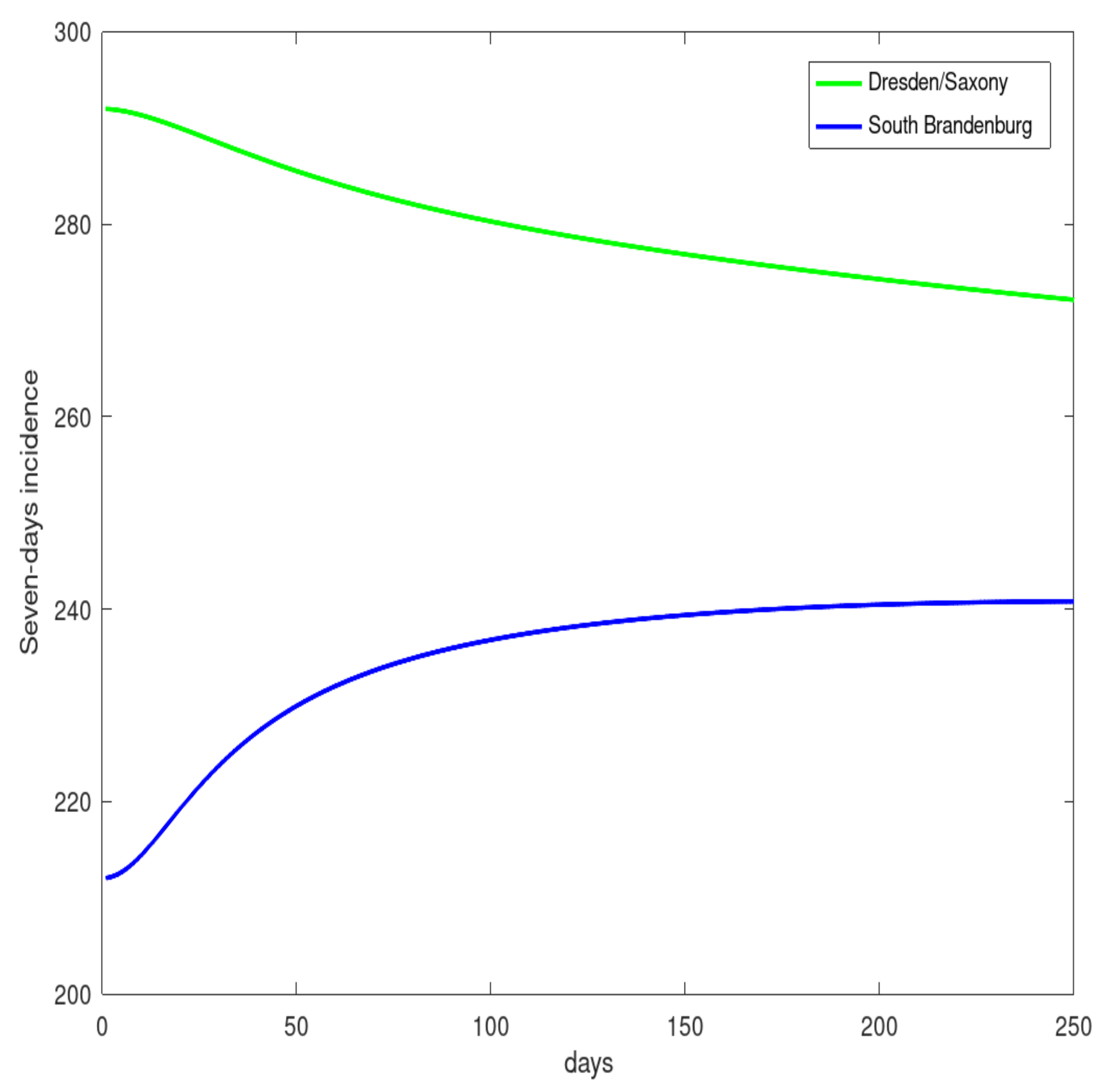
However, regardless of these uncertainties, one can obtain information about the pandemic propagation, for example, the influence of hot-spots of high incidences (Saxony) to regions with low incidences (for example, South of Brandenburg).

3. Data of the Different Federal States of Germany

At the beginning of the year 2021 (14th of January), the Robert Koch Institut (RKI), being responsible for the daily COVID-19 data collection, published the seven-day incidence data (of January the 14th, 2021 [8]), summarized in Table 1. The values of Table 1 are used as initial data for the function $s_0$ of Equation (2).

The data in Table 1 are used as a base for the determination of the diffusion coefficient function.

4. The Numerical Solution of the Initial Boundary Value Problem

Based on the subdivision of $\mathsf{\Omega }$ (area of Germany) into finite rectangular cells ${\omega }_j,j\in I_{\mathsf{\Omega }}$, where $I_{\mathsf{\Omega }}$ is the index set of the finite volume cells, and $\mathsf{\Omega }={\cup }_{j\in I_{\mathsf{\Omega }}}{\omega }_j$, Equation (1) was spatially discretized with a finite volume method. Along with the discrete boundary condition Equation (4), one gets a semi-discrete system continuous in time

$$\frac{\partial s_j}{\partial t}={\nabla }_h·\left(D{\nabla }_h{s}_j\right)+q_j,j\in I_{\mathsf{\Omega }},$$

(7)

where the h indicates the discrete version of the ∇-operator. The finite volume method is of a spatial order two; see, e.g., [18]. The time discretization is done with an implicit Euler scheme of order one. This allows us to work without strict restrictions for the choice of the discrete time-step ${\Delta }_t$. At each time-level, one has to solve the linear-equation system,

$$\frac{1}{{\Delta }_t}{s}_j^{n+1}-{\nabla }_h·\left(D{\nabla }_h{s}_j^{n+1}\right)=\frac{1}{{\Delta }_t}{s}_j^n+q_j,j\in I_{\mathsf{\Omega }},$$

(8)

for $n=0,\dots ,N,N=(T-t_0)/{\Delta }_t$. $s_j^0$ was set to the incidence $s_0\left(x\right)$ for $x\in {\omega }_j$, $j=1,\cdots ,I_{\mathsf{\Omega }}$.

Due to the complex geometry of the region $\mathsf{\Omega }$ with the Jacobi method, an iterative solution method for Equation (8) of the form $A\mathbf{s}=\mathbf{b}$ was used. The coefficient matrix A is irreducibly diagonal dominant, and therefore, the convergence of the Jacobi-iteration method arises. For the discretization parameters, ${\Delta }_t$ values in the range of 0.1 to 1 day were chosen. The 2-dimensional spatial discretization parameters ${\Delta }_x$ and ${\Delta }_y$ range 7 to 14 km. With those discretization parameters, seven to twelwe Jacobi-iterations are necessary to comply with the criterion (Euclidian norm of the relative error),

$$\frac{\left|\right|s^{n+1,i+1}-s^{n+1,i}{\left|\right|}_2}{\left|\right|s^{n+1,i}{\left|\right|}_2}<ϵ$$

for $ϵ={10}^{-4}$.

5. The Qualitative Behavior of the Diffusion Model

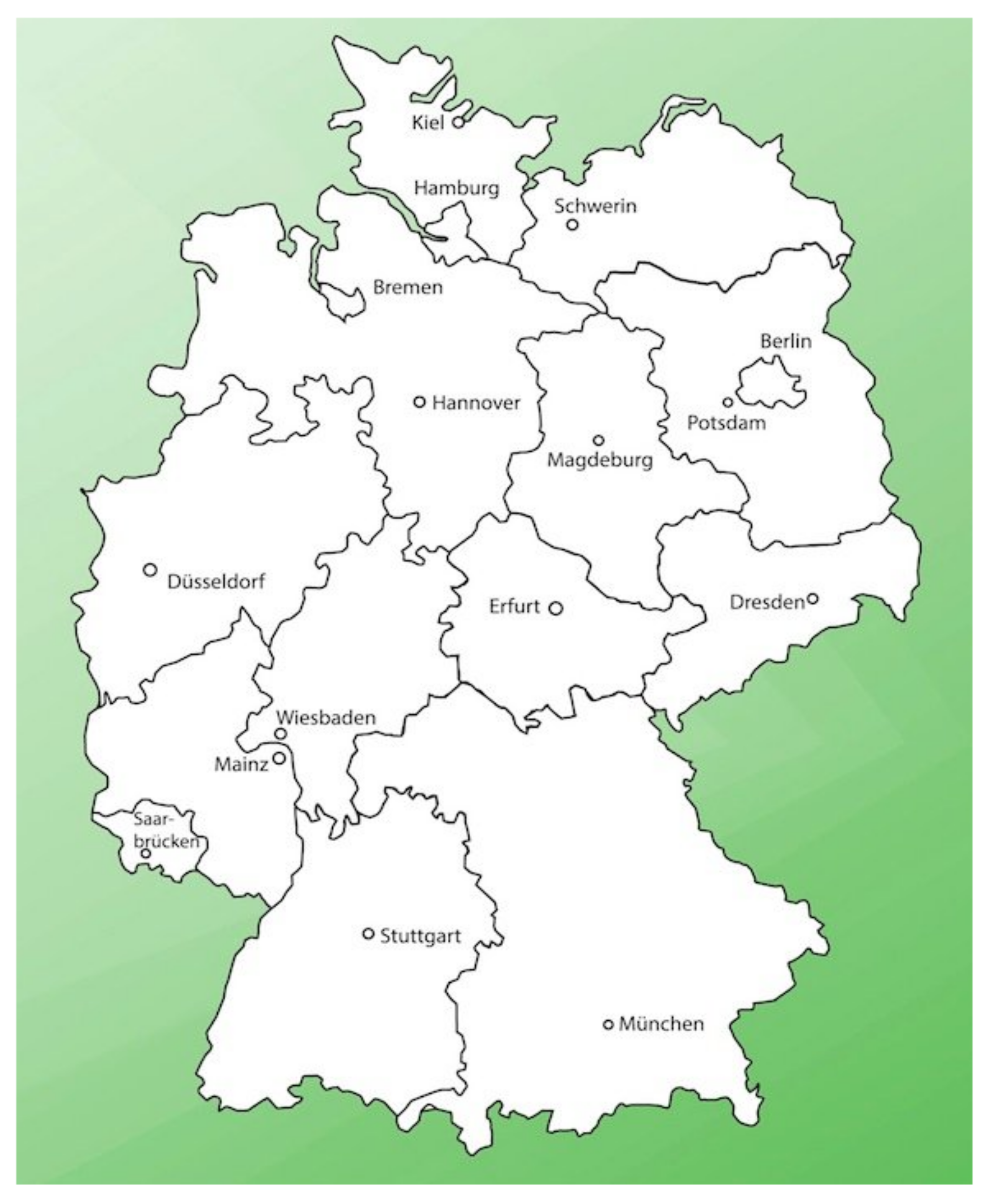
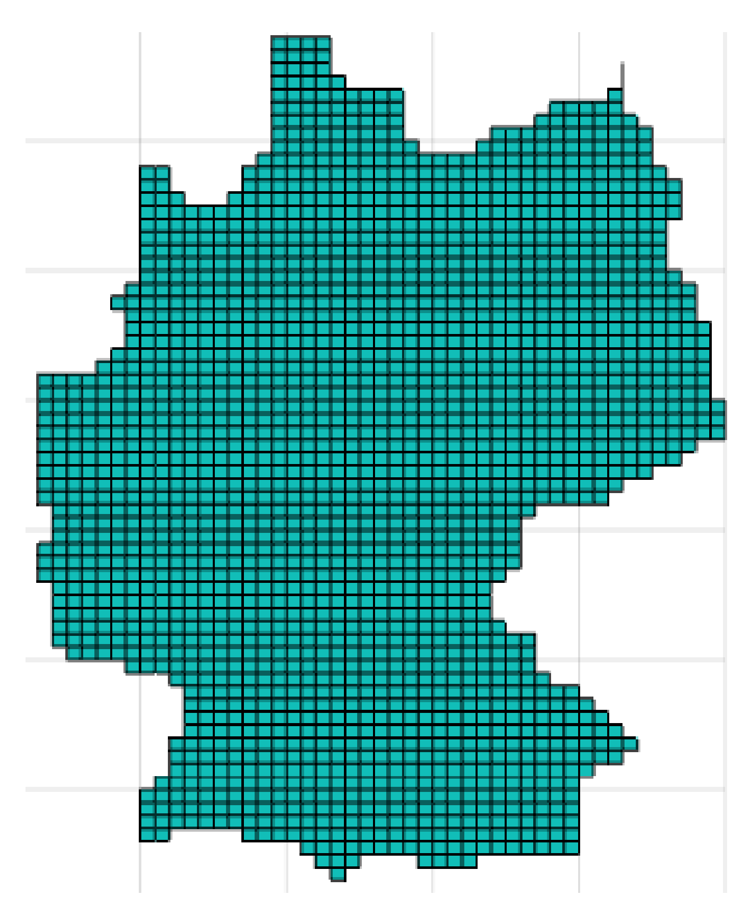
Figure 1 shows the map of Germany. For the sake of simplicity, the German border is approximated by a simple polygon. In Figure 2, the region $\mathsf{\Omega }$ is adumbrated, the size of the finite volume cells, ${\Delta }_x\times {\Delta }_y\approx (8\times 8){\mathrm{km}}^2$.

To validate the numerical method for the diffusion setting, a test to be made in order to reach a steady-state, i.e., the equilibrium given by Equation (6). One can use large time-steps (of 10 days) as soon as ther is no need to follow any time behavior here. With the seven-day-incidence of 12 January 2021 for the German federal states, gets the result $s\approx 160=\mathrm{const}.$ on $\mathsf{\Omega }$. This is the constant value, which is evaluated using Equation (6). It should be noted that this steady-state computation is only done for the validation reasons of the conservative approximation of the continuous mathematical model by the numerical finite-volume approximation. However, it is important to stress that a long-term simulation of more than a year is necessary to approach the steady-state. This is also a hint that the diffusion is a very slow, long-scale process.

For the time-behavior simulations, let us start with the case $q=0$. ${\Delta }_t$ is then set to a half-day. Figure 3 displays the initial state. The initial state is a piece-wise constant function with values of the seven-day incidence of the 16 federal states where Munich is considered as a town with over a million inhabitants taken separately as it was excluded from Bavaria.

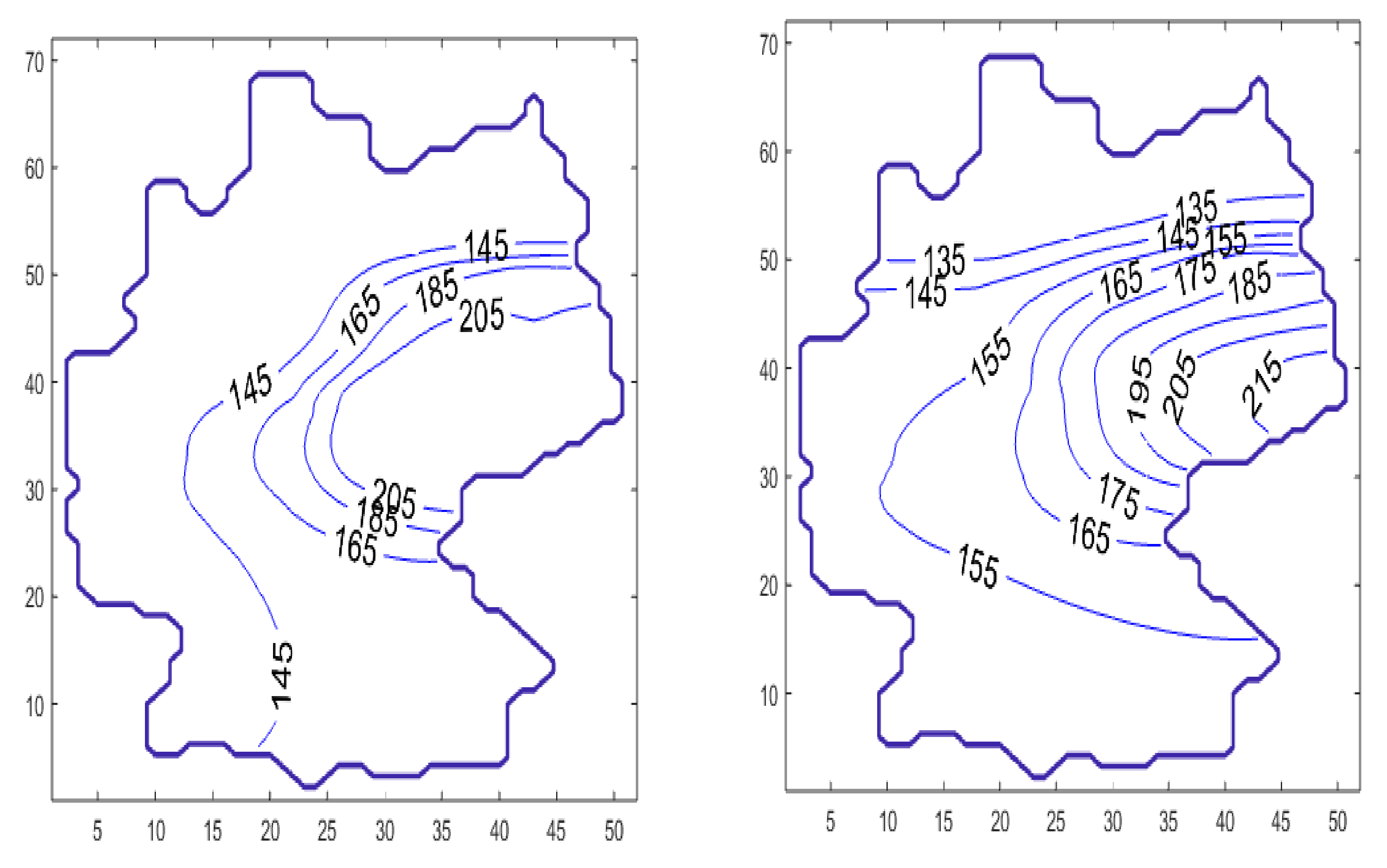
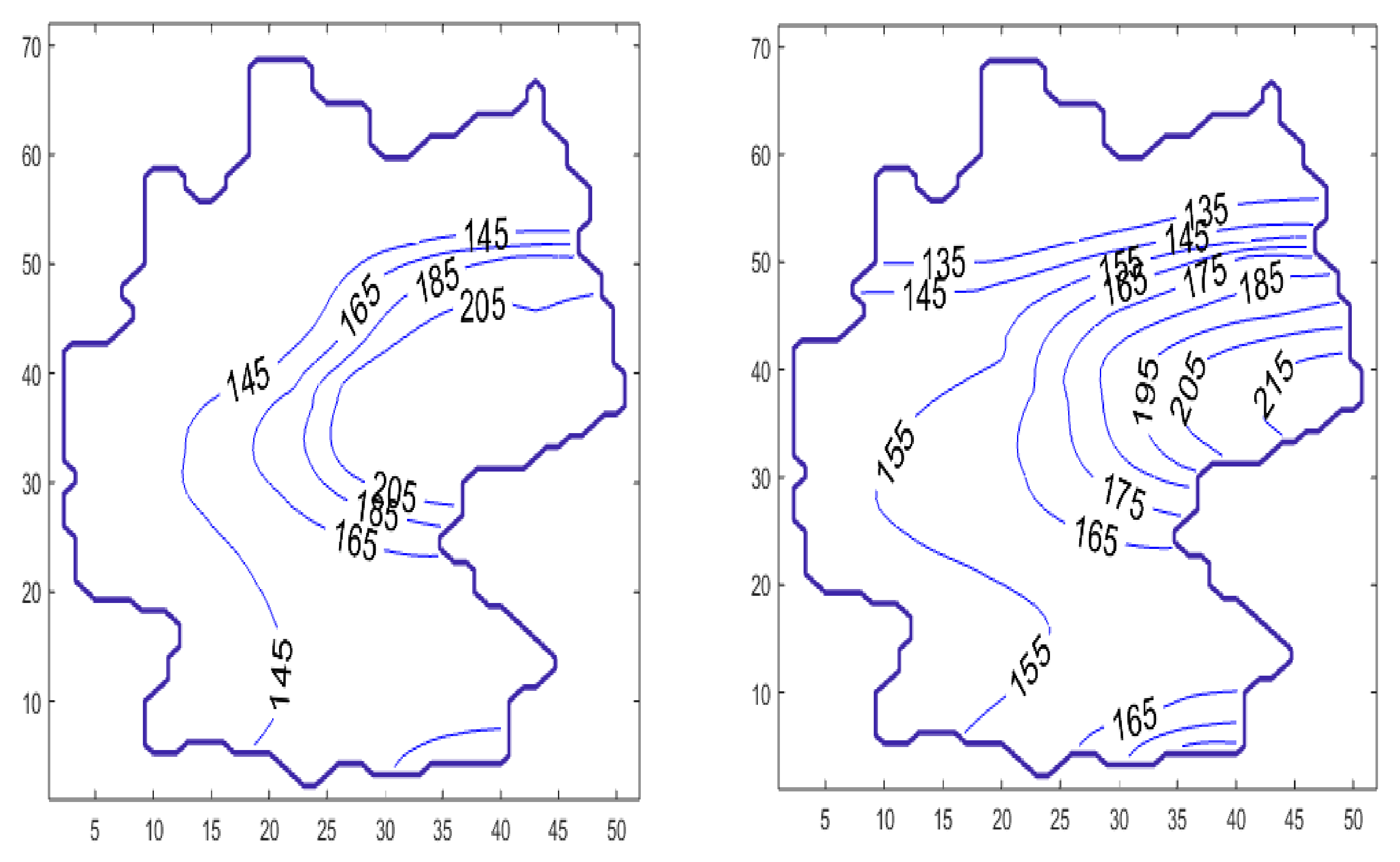
Figure 4 shows the development of the diffusion process with the change in contour lines of s of the levels 135, 155, 175, 195, and 215 over a period of 100 days. Especially in the border regions (Saxony—Brandenburg, Saxony—Bavaria, Saxony—Thuringia), one can observe a transfer of incidence from the high level incidence of Saxony to the neighbored federal states. Furthermore, the high incidence level of Berlin was transferred to the nearby Brandenburg region. The north states with a low incidence level were only influenced by the other states weakly. A typical smoothing and decreasing of the incidence gradients can also be observed. The short-horizon forecast confirms the qualitative development of the incidence in Germany. A finer resolution of the incidence propagation will be considered below by finer modeling of the source-sink term q.

In Figure 4, the development of the seven-day incidence of a high incidence region (Dresden) compared to a low incidence region (South Brandenburg) is shown. With the parameters $\alpha$, $\beta$ and $\gamma$ of the boundary condition Equation (3), it is possible to describe several situations at the borders of the boundary $\mathsf{\Gamma }$ of $\mathsf{\Omega }$. The case with $\alpha =0$, $\beta =-D$ and $\gamma \ne 0$ describes a flux through the border. Such scenario is used in the following example to describe the way home of people with COVID-19 from Austria to Bavaria.

The boundary condition at the border crossing reads:

$$-D\nabla s·\overrightarrow{n}=\gamma .$$

The initial state $s_0$ the same as in the example above. $\gamma >0$ means an ”inflow” of people with COVID-19, $\gamma <0$ indicates a loss of people with COVID-19, while $\gamma =0$ refers to a closed border. In Figure 5, the move of the contour lines of s for the case $\gamma =250$ km/day is shown.

At the south border of Bavaria, one can observe the increase of s caused by the flux of s from Austria to Bavaria.

The results without a source-sink-term ($q=0$) describe the qualitative trend, which was observed in the pandemic development. To describe the whole pandemic process of long-scale diffusion and the small-scale local virus transmission, it is necessary to consider local epidemic spreading models, as it is done in the next Section.

6. Consideration of the Local Transmission via a SIR-Model in the Diffusion Model

The previous section demonstrates the diffusion as a long-scale process. On the other hand, a small-scale process occurs with the direct virus transmission via epidemiological infection. This process can be described with a SIR-model, for example.

The change of s per day can be divided into a part coming from diffusion and another part coming from the local passing of the virus. The second issue will be modeled with the SIR-model. The local virus transmission means, in other words, the consideration of an SIR-model in the federal states of Germany separately. The SIR-model is defined by the following system of equations (see, e.g., [1,19]):

$$\begin{array}{ccc}\hfill \frac{d{S}_j}{dt}& =& -{\kappa }_j\frac{I_j}{N_j}{S}_j,\hfill \end{array}$$

(9)

$$\begin{array}{ccc}\hfill \frac{d{I}_j}{dt}& =& {\kappa }_j\frac{I_j}{N_j}{S}_j-{\eta }_j{I}_j,\hfill \end{array}$$

(10)

$$\begin{array}{ccc}\hfill \frac{d{R}_j}{dt}& =& {\eta }_j{I}_j,\hfill \end{array}$$

(11)

where j defines the respective federal state, and $S_j$, $I_j$ and $R_j$ are the groups of susceptible, infected and recovered people. $N_j$ is the population of the respective federal state. $\eta$ is the reciprocal value of the typical time from infection to recovery ($\eta =1/14\approx 0.07$). ${\kappa }_j$ is the average number of contacts per person per time multiplied by the probability of disease transmission for a contact between a susceptible and an infectious subject.

Instead of Equations (9) and (10), one also considers the stochastic differential equations (SDEs):

$$\begin{array}{ccc}\hfill d{S}_{j_t}& =& -{\kappa }_j\frac{S_{j_t}}{N}{I}_{j_t}dt-\nu I_{j_t}d{W}_t\hfill \end{array}$$

(12)

$$\begin{array}{ccc}\hfill d{I}_{j_t}& =& ({\kappa }_j\frac{S_{j_t}}{N}{I}_{j_t}-\eta I_{j_t})dt+\nu I_{j_t}d{W}_t\hfill \end{array}$$

(13)

$$\begin{array}{ccc}\hfill d{R}_{j_t}& =& \eta I_{j_t}dt.\hfill \end{array}$$

(14)

Here, $I_{j_t}$, $S_{j_t}$ and $R_{j_t}$ denote stochastic processes, and $W_t$ is a Wiener process with its main characteristic, $W_t-W_s\sim N(0,\sqrt{t-s})$, $t>s$, and the independence of $W_t$ and $W_s$ for $t\ne s$. With the addend $\nu I_{j_t}d{W}_t$, one can describe random fluctuations of people with COVID-19, for instance, unrecognized or over/under-estimated people with COVID-19. The scope of such random effects can be controlled by the parameter $\nu$.

The relation between the actual reproduction number, $\mathcal{R}$, and $\kappa$ and $\eta$ is $\mathcal{R}=\kappa /\eta$.

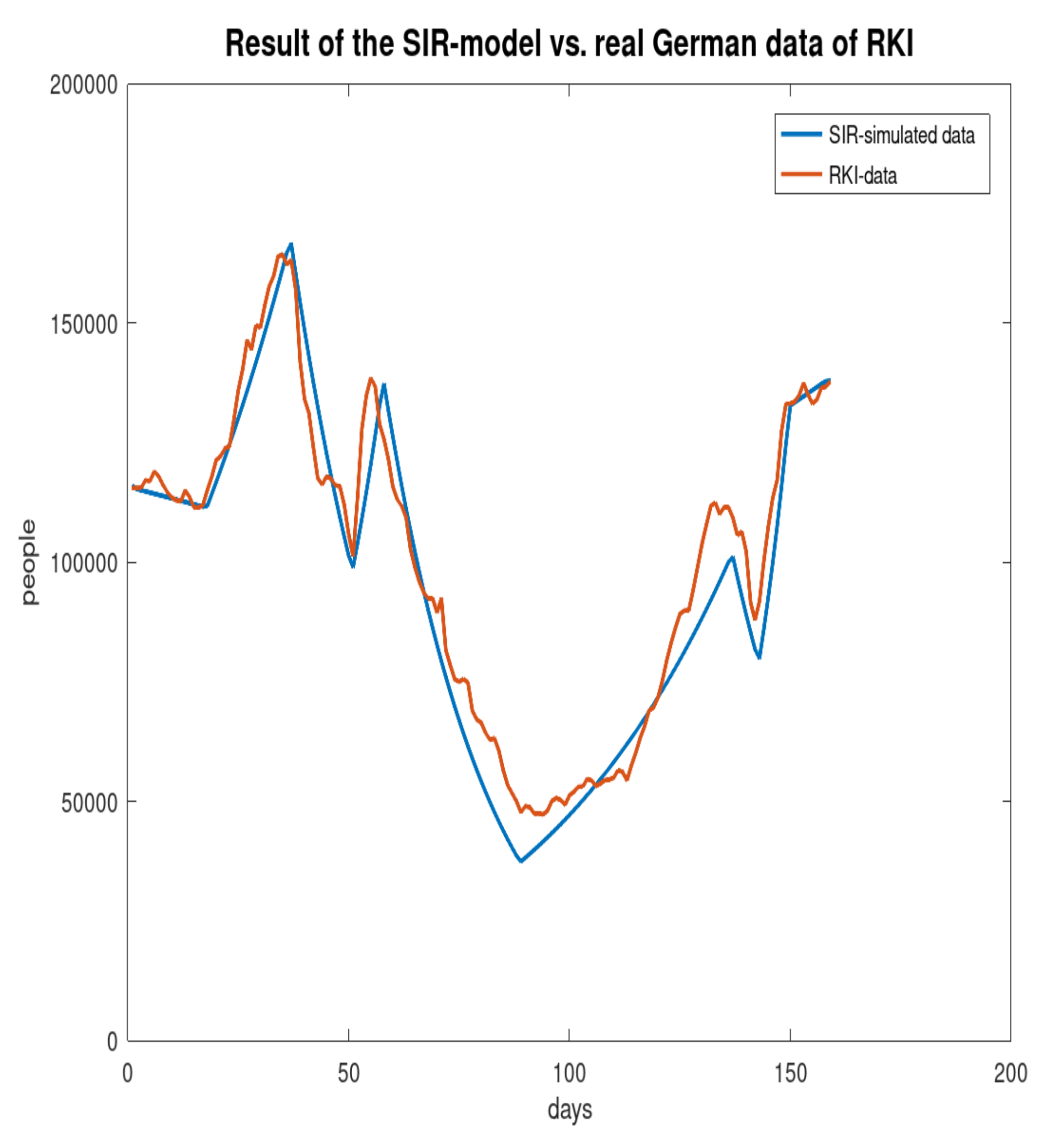
To clarify about a possible relation between actual non-pharmaceutical measures of the government and the values of $\kappa$ (or $\mathcal{R}$), let us consider the development of people with COVID-19 in the period from 18 November 2020 to 24 April 2021.

Figure 6 shows the RKI data [8] and the result of the simulation with the SIR-model. The curve shows the implication of the drastic changes of the measures by the politicians with a sequence of local minimums followed by local maximums. The first local minimum seen was reached on December the 5th, the first local maximum found was on December the 24th, the next minimum found was on 7 January 2021, and the next local maximum was on January the 14th. In

Table 2. Simulated period-depending average number of contacts per persone per time, $\kappa$, and actual reproduction number, $\mathcal{R}$, for Germany.

Period	$\mathit{\kappa }$	$\mathcal{R}$
18 November 2020–23 November 2020	0.068	0.97143
24 November 2020–6 January 2021	0.92	1.3143
7 January 2021–13 January 2021	0.12	1.7143
14 January 2021–13 February 2021	0.028	0.4
14 February 2021–2 April 2021	0.092	1.3143
3 April 2021–8 April 2021	0.028	0.4
9 April 2021–15 April 2021	0.1464	2.0914
16 April 2021–24 April 2021	0.076	1.0857

, the possible values of $\kappa$ to obtain the curve of the people with COVID-19 for the simulation with the SIR-model are shown. The possible $\kappa$-values for the chronological periods are obtained with a simple trial-and-error method.

The measures of the government from the end of April 2021 can be compared with the measures of the period beginning at the 14th of January with a $\kappa$-value of $0.028$. For the propagation of the pandemic from April the 25th, this $\kappa$-value is used. Due to the fact that the measures of the government are based on the infection control law, which are valid from 25 April 2021, the same $\kappa$-value is used for all federal states of Germany.

In what follows, the diffusion model (1), (2), (4) coupled with the SIR-model (9)–(11) is used.

To take into account the long-scale and small-scale processes, one considers, after the diffusion steps with the size ${\Delta }_t$, the model (9)–(11) for a time-interval ${\Delta }_t$. This means to solve a family of initial value problems in the interval $[t_p,t_p+{\Delta }_t]$ in every diffusion step of Equation (8) from $t_p$ to $t_p+{\Delta }_t$ (see Algorithm 1). The initial values for $I_j\left(t_p\right)$ are used as the mean values of s (Table 1) of the respective federal states. The first values of $R_j\left(t_p\right)$ (in the first diffusion step) are set to zero and the $S_j\left(t_p\right)$ values come from the relation $N_j=S_j+I_j+R_j$. The result of the initial value problem $I_j(t_p+{\Delta }_t)$ is converted to $s_j(t_p+{\Delta }_t)$ and used to determine q for Equation (8) by the changing rate of $s_j$, which means

$$q(x,t_p+{\Delta }_t)=\frac{s_j(t_p+{\Delta }_t)-s_j\left(t_p\right)}{{\Delta }_t},x\in {\omega }_j,$$

during the time ${\Delta }_t$, caused by the process modeled with the equation system (9)–(11). In the deterministic case ($\nu =0$), the Euler method is used to solve the initial value problem per diffusion time-step (with a time-step of ${\delta }_t={\Delta }_t/10$). For constant coefficients $\kappa$, $\eta$ there are possibilities of finding analytic solutions of the SIR-system, which can be found in [20,21]. However, for time-dependent coefficients, numerical methods to be used to find a solution. If $\nu \ne 0$ (stochastic case), the SDE system (12)–(14) is solved using the Milstein method [22]. Here, it is important to note that the step-sizes ${\Delta }_t$ and ${\delta }_t$ used are chosen heuristically. Let us note that the analysis of the physics of time-scales of both the local transmission and the diffusion process is an interesting point and should be considered in further investigations of such combined modeling together with the parameters of the diffusion process; see, e.g., [23].

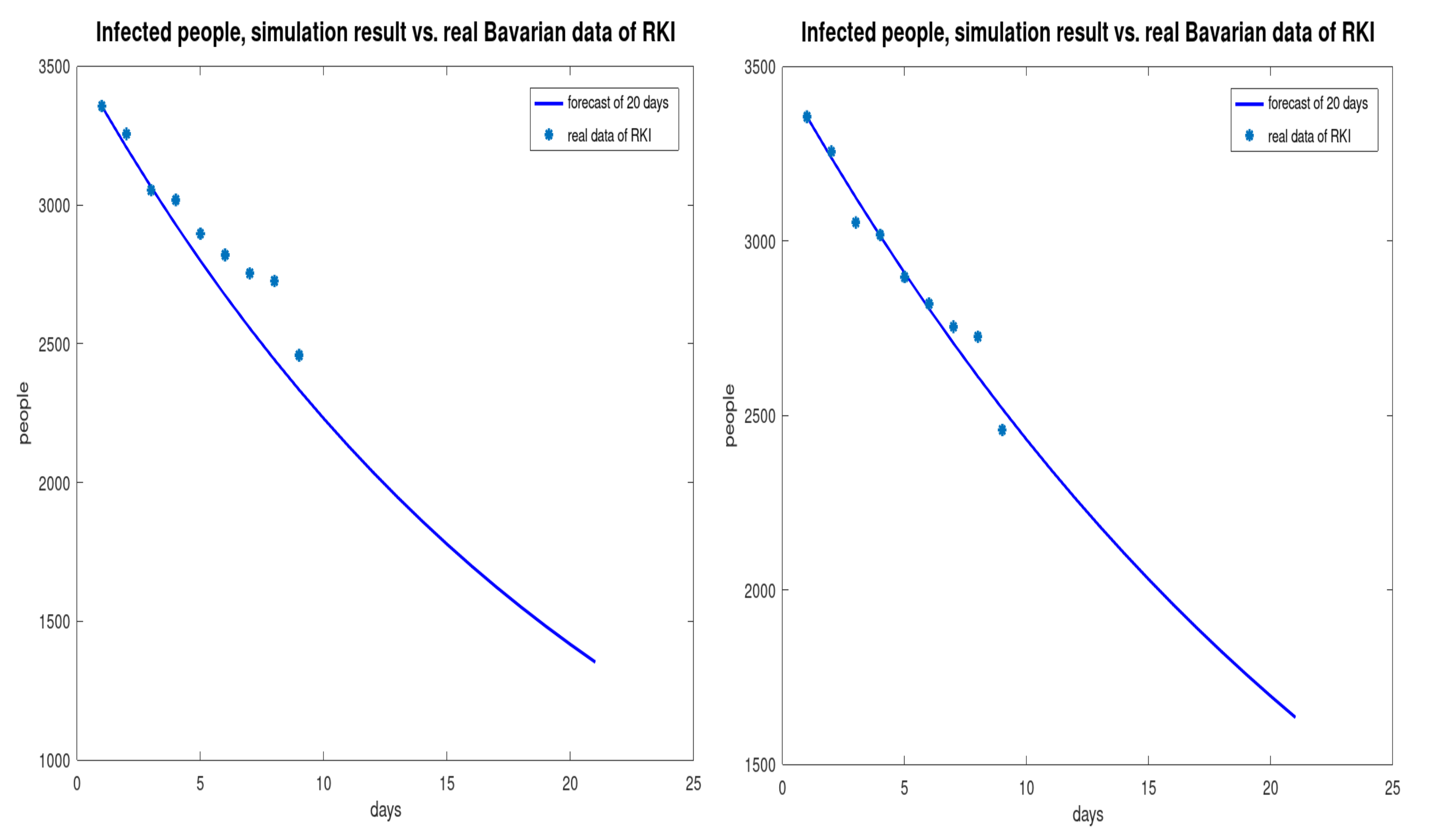
Due to the poor informativeness of surface graphs and contour lines, the propagation of the people with COVID-19 in Bavaria is used to compare the simulated results with the real data of the RKI. The result of the diffusion model coupled with the stochastic SIR-model ($\nu =0.25$) over the period of April 26th to May 5th is shown in Figure 7 (${\Delta }_t=1\mathrm{day}$, ${\delta }_t={\Delta }_t/10$). In addition, to the nine days where the real data are known, a forecast up to the 16th of May 2021 is made.

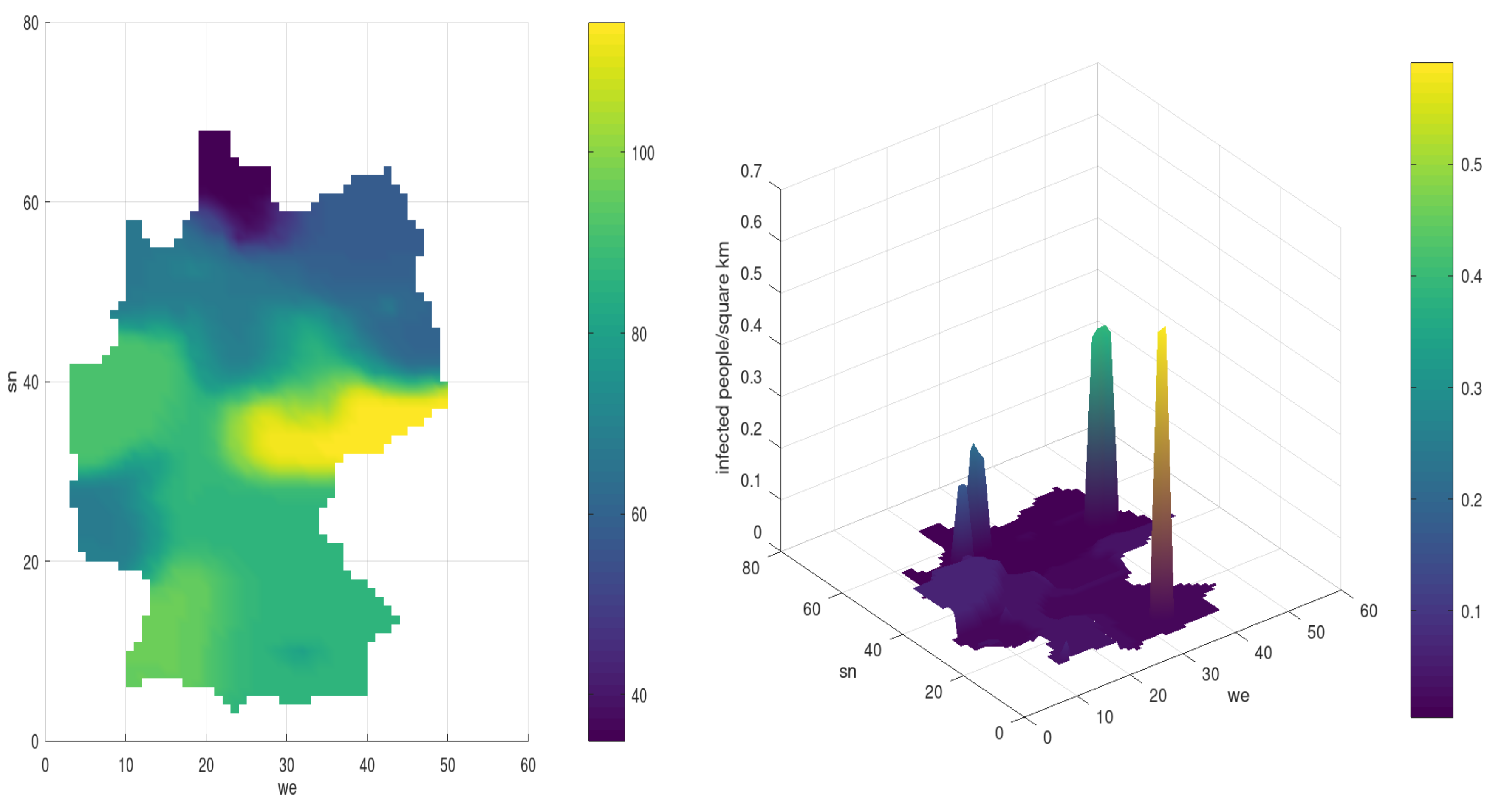
For the reinterpretation (by counting back using the people densities and the area of the federal states) of the result for the seven-day incidence, in Figure 8 the incidence with the congruous distribution of the people with COVID-19 per square kilometer is considered. It is obvious that the people with COVID-19 are concentrated in the congested urban and metropolitan areas such as Munich, Hamburg, Berlin, and Ruhr.

Algorithm 1 Diffusion model coupled with the SIR-model.

for j = 1, …, M, diffusion time-steps do  Initialization: Inhabitants, density, aread data of the federal states, model parameter  for i = 0, …, N−1, SIR time-steps per diffusion time-step do   for k = 1, …, 17, number of federal states added by Munich do    Local transmission of the pandemic in state k, development of people with COVID-19, integration of Equations (12)–(14)   end for  end for  Determination of the source term q using the change rate of people with COVID-19 Solution of Equation (8) end for

7. Discussion and Conclusions

The numerical simulations show an impact of diffusion effects on the propagation of the COVID-19 pandemic. Specifically, the observed influence of high incidence regions of Saxony and Bavaria on neighbored regions could be confirmed with the diffusion concept. It must be remarked that these processes are very slow compared to the virus transmission in a local hot-spot cluster. However, with the presented model, it is possible to describe the creeping processes that occur alongside slack measures like inadequate lock-downs.The model is convenient to embrace the important issue of border traffic and its influence on the pandemic.

The situation in Germany up to February 2021 showed a tendency to a seven-day incidence, which is approximately constant and is consistent with the property of the diffusion model to gravitate to equilibrium, provided that there is no essential flux through the borders. However, this a snapshot of the pandemic dynamics only. If the reproduction number, $\mathcal{R}$, fluctuates around one, the pandemic development is not really stable (this behavior can be approximated with the stochastic SIR-model). Small changes in the aggressiveness of the SARS-Cov-2 virus could lead to an exponential growth of the incidence.

With the approach of the source-sink function, q, using SIR-models, the small-scale and long-scale effects could be recorded, and the model could be improved from a qualitative to an approximately quantitative description of the incidence development.

It should not be concealed that the horizon of the forecast should be limited because of the very dynamic propagation of the pandemic; for example, considering the virus mutants from the United Kingdom, Brazil and South Africa. Therefore, it is necessary to update parameters such as the average number of contacts per person per time, $\kappa$, or the weight of the small-scale influence. The presented model is qualified to adjust for such new constellations very quickly.

The presented model proved to be a valuable instrument to trail and forecast the pandemic. There are some possible extensions of this model; for example, the further subdivision of the relevant population into more than three compartments. The group of exposed (vulnerable), quarantined or vaccinated people could be considered as further compartments, for instance.

It is necessary to emphasize that the seven-day incidence is not the only meaningful measured value. If large-sized regions, areas, and administrative districts with a small population density are compared to a small-sized region with a great population density, the data must be interpreted carefully. If the seven-day incidences are equal, the pandemic situation in the administrative district is more complicated than in the region with the small population density. This should be respected, and the incidence value can not be the only criterion for the decisions of the politicians and physicians to manage the pandemic.

In addition to a large-scale vaccination of the population (herd immunity), the most effective non-pharmaceutical measure to contain the pandemic is the reduction of contact, leading to the decrease in the parameter $\kappa$.

Regarding the often skeptical discussions of the mathematical modeling of the spread of the pandemic and the predictions made, it must be said that the results and views of mathematicians, physicists and other natural scientists are contributions and should only be taken as recommendations and advice. At best, dramatic developments do not occur because of the policy decisions made following the advice and recommendations of scientists.