Faraday’s Law and Magnetic Induction: Cause and Effect, Experiment and Theory


1
Physics Department, Lancaster University, Lancaster LA1 4YB, UK
2
Cockcroft Institute, Keckwick Lane, Daresbury WA4 4AD, UK
Physics 2020, 2(2), 150-163; https://doi.org/10.3390/physics2020009
Submission received: 18 March 2020
/
Revised: 21 April 2020
/
Accepted: 27 April 2020
/
Published: 6 May 2020
(This article belongs to the Section Physics Education)
Abstract
:Faraday’s Law of induction is often stated as “a change in magnetic flux causes an electro-motive force (EMF)”; or, more cautiously, “a change in magnetic flux is associated with an EMF”. It is as well that the more cautious form exists, because the first “causes” form can be shown to be incompatible with the usual expression , where is EMF, is a time derivative, and is the magnetic flux.This is not, however, to deny the causality as reasonably inferred from experimental observation—it is the equation for Faraday’s Law of induction which does not represent the claimed cause-and-effect relationship. Unusually, in this induction scenario, the apparent experimental causality does not match up with that of the mathematical model. Here we investigate a selection of different approaches, trying to see how an explicitly causal mathematical equation, which attempts to encapsulate the experimental ideas of “a change in magnetic flux causes an EMF”, might arise. We see that although it is easy to find mathematical models where changes in magnetic flux or field have an effect on the electric current, the same is not true for the EMF.
1. Introduction
Michael Faraday was the first person to publish experimental results on electromagnetic induction, a phenomenon which is frequently described as a current being induced when the magnetic flux through a conducting coil is changed.
The phenomenon is compactly described by a mathematical model relating the “electro-motive force” (EMF) around a closed circuit to the temporal changes in magnetic flux —the integral of the magnetic field over the surface delineated by that closure. Faraday’s law of induction can be directly related to the Maxwell–Faraday vector equation ([1], p. 160). Using the notation where , the equations are written as
where is electric field and is magnetic field.
However, a fundamental law of causality demands that effects cannot occur before their causes; and this expectation has mathematical consequences. These consequences give rise in particular to the famous Kramers-Kronig relations [2,3,4], which can be used to constrain both the spectral properties of physical quantities and the models used to describe them.
Here we take a local view of causality, rather than a global one, and use the time domain most natural to expressions of causal behaviour. In this case a scheme exists [5] for attributing specific cause and effect roles to the components of mathematical models that are based on temporal differential equations (for mathematical details see also [6,7].) Most simply, this means that in any equation of the mathematical model it is the highest-order time derivative term which is to be regarded as the effect, with the other terms as causes; but note that it can also be applied to systems of coupled equations (e.g., Maxwell’s equations ([5], Section V), as well as later in this paper in Section 5.2). As a simple example, since Newton’s second law can be written as , then according to [5], we can state that the force causes a change in the velocity of a mass m. The use of this interpretation is particularly natural when considering the computational solution of dynamic physical models; see Appendix A in [8], and where the main focus of attention is what happens as the current state of the system is updated [9,10] (i.e., integrated forwards in time), or as the universe extends itself into its “future” (as in, e.g., the causal set approach [11]).
Note that other discussions of and approaches to causality in electrodynamics relevant to Faraday’s Law do exist [12,13,14]. In particular, one significant school of thought prefers to relate everything back to the original source terms (see, e.g., [12], and remarks in Appendix B of [8]). Unfortunately, since Faraday’s Law contains no explicit references to source charges, we cannot analyse it in regards to cause and effect on that basis—we would need a different model that did refer to the source charges and their motions (e.g., see [15]).
Consequently, in what follows we choose to only use the local and Kramers-Kronig compatible definition [5] for what constitutes a causal interpretation of a mathematical model.
Using the local view of causality described in [5] and in Box 1, since Equation (1) has no time derivatives applied to , but one time derivative applied to , this means that the EMF must be considered a cause, where the change in flux is its effect. As a consequence, it would be more intuitive to rewrite Equation (1) instead as
where we are likewise compelled to describe the spatial gradients of the electric field as a cause, and the resulting temporal changes in field as its effect. Somewhat disturbingly, this now means we are unable to interpret our mathematical model of Faraday’s law of induction as our preferred causal statement: i.e. where changes in flux induce an EMF (and hence drive currents) [16,17,18]. However, based on our mathematical model, we are still able to make the weaker statement where the two are merely equated or associated with one another [19].
This situation suggests that Equation (2), despite its utility, is simply not a good causal representation of the experiment we had in mind. To resolve this we need to to make a clear distinction between the causality apparent in an experiment, and the causal interpretation of the mathematical model that is, necessarily, only an approximation to that experiment. While we would usually hope that these agree, it seems that in the case of Faraday’s law they do not, and in Section 2 we discuss why (or how) this can be.
Clearly, it would be desirable for our mathematical description of induction to explicitly show how EMF or electrical current could be generated in a conductor, whether by the varying properties of the magnetic field, or by motion of the conductor within those fields. In what follows we try three (non-relativistic) approaches to finding a mathematical model which describes how some property or behaviour of the magnetic flux (or perhaps just the magnetic field) is explicitly attributable as being the cause of an EMF.
The first, in Section 3 is based on the Maxwell–Faraday equation, and fails. The second, in Section 4, is based instead on the Maxwell–Ampere equation, and achieves that essential goal, but perhaps not in a very satisfactory way. The third, in Section 5, is based on the Lorentz force law, and we try both a simple abstract calculation as well as a specific setup, common in many undergraduate courses, and derive a model for the current due to magnetic fields and motion. Finally, in Section 6, we conclude.
Box 1. How to be causal: Consider the simple model equation , which under the interpretation used here is interpreted as “Q causes changes in R”. Using the mathematical definition of the derivative, at some arbitrary time the model equation is
Just before we take the limit, and for some small enough value of , we have
Now let us try to use this as a predictor of the future. We immediately see that the latest-time (or most future-like) quantity is , so we rearrange to put this on the left, and get
Here, we see that to update our knowledge of R to its next value at requires (a) past knowledge of R (i.e., ) and (b) current knowledge of Q (i.e., )). Thus it is clear that the value of Q causes changes in R. If we instead wanted to calculate Q, hoping to say something like “R causes Q”, we would first rearrange Equation (4) into
but will immediately see that depends on a future value of R, namely – and a dependence on future values is incompatible with standard notions of causality.
This undergraduate level presentation discussing magnetic induction highlights the distinction between any inferred experimental causality and that encoded in its mathematical model. It shows that the apparently useful definition of an EMF actually works against our attempts to generate a model where it is induced by changes in magnetic flux. In contrast, an alternative focus on the electrical currents generated by motion and or magnetic field variation has no such limitations.
2. Experiment
Consider an example experiment consisting of two pieces of apparatus, (i) a magnet, and (ii) a loop or coil with a voltmeter attached, as depicted in Figure 1. When we move the magnet in the vicinity of the loop, we see a voltage induced. On the basis of this experimental experience, it is therefore quite natural—and indeed accurate—to infer that moving the magnet caused a voltage (or EMF) appear. If also a student of physics, we might then also relate the motion of the magnet to the amount of magnetic flux crossing the loop, and so say our experiment indicates that “a change in flux causes an EMF”.
The “experimental causality” just described is not controversial. However, what is under examination here is the conflation of this experimental experience of causality with any causal interpretation of the mathematical expression of Faraday’s Law, i.e., Equation (2).
For a better understanding we need to start by being clearer about why we might deduce that the voltage was caused by our actions in moving the magnet. Notably, we should realise that this is not merely because we saw a finite voltage registered on the voltmeter, since it might simply have been poorly zeroed and always have some finite reading, or offset by the effects of some external field irrelevant to the induction experiment. Instead, we say “caused” because after (and as) we moved the magnet near the loop, the voltage registered by the voltmeter changed. The change in voltage is the visible effect that leads us to look for its cause. At the very least, then, we should want our causal model of induction to describe how changes in voltage (“EMF”) occur due to external stimuli.
Let us now try to mathematically codify our experiment, allowing for the pre-defined input (the motion of the magnet), while looking for the resulting effect on the output (the EMF ). Assuming for simplicity a fixed-strength magnet, with an equally fixed orientation, the sole input to our model only needs to be its velocity . This is the cause; it is something we specify in the experimental design and then implement. We are hoping, or expecting, this cause to give rise to a change. This change should be visible as an effect on the measured EMF, so that at one moment it might be zero, but the next it will be different, i.e., it should change with time, and somehow as a result of the cause . Thus we might write
where is a function or operator understood to contain all the necessary information about electromagnetism, the field pattern produced by the magnet, the Lorentz force law on charges, and circuit theory.
We can at a glance now see that the structure of the mathematical model Equation (7) for our experiment is not of the same form as Faraday’s Law: Equation (2) only explicitly refers to changes in flux , and not to changes in EMF. Indeed, this should not need be surprising, since Equation (2) is not even an attempt at a microscopic model of the experimental process, where the moving magnet produces a changing electromagnetic field distribution, which then goes on to influence the motion of electrons, producing or changing electrical currents (e.g., [15]), and thus subsequently giving rise to an EMF. Since so much experimental detail is omitted from Equation (2), it is not at first sight clear why we should expect the two to match at all, let alone perfectly.
Nevertheless, in what follows we will attempt to find a Faraday-like law that matches better to our experimental concept.
3. Maxwell–Faraday Equation
First let us consider the standard derivation of Faraday’s law of induction starting with the curl Maxwell’s equation; note however some approaches take the reverse approach, and start with induction and reduce it to the curl equation.
We start with a loop of material, and regard that loop as the boundary C of some enclosed surface S, and treat the electric field and magnetic field as shown in Figure 2. The derivation proceeds by starting with the Maxwell–Faraday equation, taking a surface integral of both sides, and then applying Stokes’ theorem to the left-hand side (l.h.s.), in order to convert the surface integral over S into a line integral over elements along C:
The causal interpretation of this equation must be [5] that the EMF “causes” changes in flux —we cannot in fact take the common interpretation that changes in flux induce (or cause) an EMF. Note that this is not an interpretation of experimental facts or observations, but one based on the mathematical model.
Further, note that the EMF, i.e., , which is supposed to represent the current-generating potential induced in the wire, is not calculated as we perhaps might have expected, i.e., by following a single charge on its path around a conducting loop to work out the voltage difference traversed. Instead what we have done is consider the forces applied to a continuous line of infinitesimal charges on the loop at a single instant, and integrated those forces. Without a model for the motion of these charges, what we have modelled is more like a dielectric ring, with bound charges and currents tied to their own locations, and not a conducting wire loop with freely moving charges and currents [20].
Of course, from a practical perspective Faraday’s Law of induction derived above and shown in Equation (1) is an exceedingly useful expression, and it is compatible with experimental measurements. Notably, in an electric motor or generator, the speed of the axle’s rotation supplies us a natural angular frequency , so that the time derivative of flux becomes a simple multiplication by ; and further, in such a quasi-stationary case, attribution of causality becomes unimportant. However, its utility is not any guarantee that it will supply a mathematical model encapsulating the casual properties that we might hope for for the generation of EMF. Neverthless, we will see later in Section 5 that this difficulty is not present when finding models that show effects on the current as a result of changes in magnetic field or flux.
4. Maxwell–Ampere Equation
In Section 3 we saw that the Maxwell–Faraday equation did not provide the causal interpretation we wanted. Consequently, let us try an alternative derivation for a model of induction starting with the curl Maxwell’s equation that represents Ampere’s Law. The aim here is to show how some suitable property of the magnetic field—hopefully related to a magnetic flux—explicitly causes an EMF to change. This would mean we can address the generation of an EMF from nothing, and use that to motivate how an induced current will appear. Since we have seen in the preceeding section that according to [5], the Maxwell–Faraday equation is the wrong way around to motivate a “magnetic fields causing (inducing) current” picture, the Maxwell–Ampere equation with its reversed roles for electric and magnetic contributions may seem more promising.
Again we take a loop containing charges, with enclosed surface S and boundary C, and treat the electric displacement and magnetic induction fields and , as in Figure 3. The derivation proceeds by starting with the Maxwell–Ampere equation, taking a surface integral of both sides, and then applying Stokes’ theorem to the right-hand side (r.h.s.) in order to convert that surface integral into a line integral:
where is the electric current.
From this we can straightforwardly see that neither an EMF or a flux emerges. However, some further thought leads us to more success by means of taking the curl of both sides before applying the surface integral. With being the permittivity, and the permeability, we have:
This equation does now give us an EMF from the l.h.s. line integral, calculated just as in Section 3. Since , and with being the speed of light, we can therefore write
This result is an induction-like equation which we can give a well defined causal interpretation where the EMF is caused: being that spatial variations in (or, when integrated, spatial variations in flux) drive changes in EMF, as do currents.
Although we could try to treat this general case, it is instructive to simplify this and take the case of zero current, and all oriented along z, and primarily aligned along and varying in the z direction so that only its component is significant. Subject to these assumptions, and calculating the effective magnetic flux as , i.e., after moving the r.h.s. surface integral through the z-direction spatial derivatives , we can write a simplified equation
As a final note, in situations where it is reasonable to replace with a , we can also recover something equivalent to the usual form, but with an extra time derivative on both sides. However, with this replacement the flux is again subjected to the highest order time derivative. Thus the induction model has also returned to the same causal interpretation—one that is reversed from our “flux as a cause” preference.
5. Lorentz Force Law
Despite the relatively familiar nature of the calculations in Section 3 and Section 4, in many ways it might be seen as more natural to derive a model of induction of current by starting with the Lorentz Force Law. Since Faraday’s Law of Magnetic Induction is not predicated on effects due to applied electric fields (see, e.g., [1], p. 160), I start with the momentum of an electric charge q in a purely magnetic field
This is in and of itself a model where changes in the charge’s momentum are caused by the (magnetic) Lorentz force . Although considering changes in momentum in the context of induced currents is unusual, in the calculations below it is a convenient way of summarizing the forces involved.
As in the previous calculations, we now hope to find it useful to define an EMF-like quantity. However, whereas those calculations derived EMF from a line integral of the electric field, here we instead base it on an integral over charges that are moving; and to emphasize this distinction we denote it rather than simply .
5.1. A Simple Loop
Here we will apply it to (one of) the charges in our conducting loop. This is a more general formulation of that in Bleaney and Bleaney ([1], p. 160), but they use it merely as a support for something equivalent to the standard calculation as done in Section 3.
Since for potential (EMF) , work W, and charge q, and work increment on a charge is given by with force along line element ,
First we line-integrate over the loop (contour ) containing charges of q and travelling at , to get the total EMF ,
Next we convert the r.h.s. line integral to a surface integral of a curl by Stoke’s theorem
so that now we can use the standard vector identity for ,
The first term vanishes since ; and we can further simplify by removing the second term if the velocity field for the charges (essentially the scaled current) has no sources or sinks. Here, for convenience, we go further and insist on a constant velocity field so that the third term also vanishes. The result is
To make this result easier to understand, we further simplify the situation as shown in Figure 4, considering a square loop in the plane, which bounds the surface S whose area S is perpendicular to the z axis. The magnetic field is oriented along z, so that the only non-zero component is , and it varies only along x, and at a fixed rate. We then move our loop sideways parallel to the x axis at a fixed speed v, so that we get a straightforward equality, but one without any time derivatives, and therefore no implied causality:
This seems most closely related to the Maxwell–Ampere formulation in Section 4, which also depends on spatial gradients of B. However, we could choose to adapt this relation by converting the numerator part of the speed , and the denominator part of the field gradient , to get
which is the normal expression of Faraday’s Law, if we assume the equivalence of and , despite their being derived from different starting points. Regardless of this, we have still failed to find a mathematical model with the causal properties we are looking for where properties of the magnetic field or its flux cause currents to appear or change.
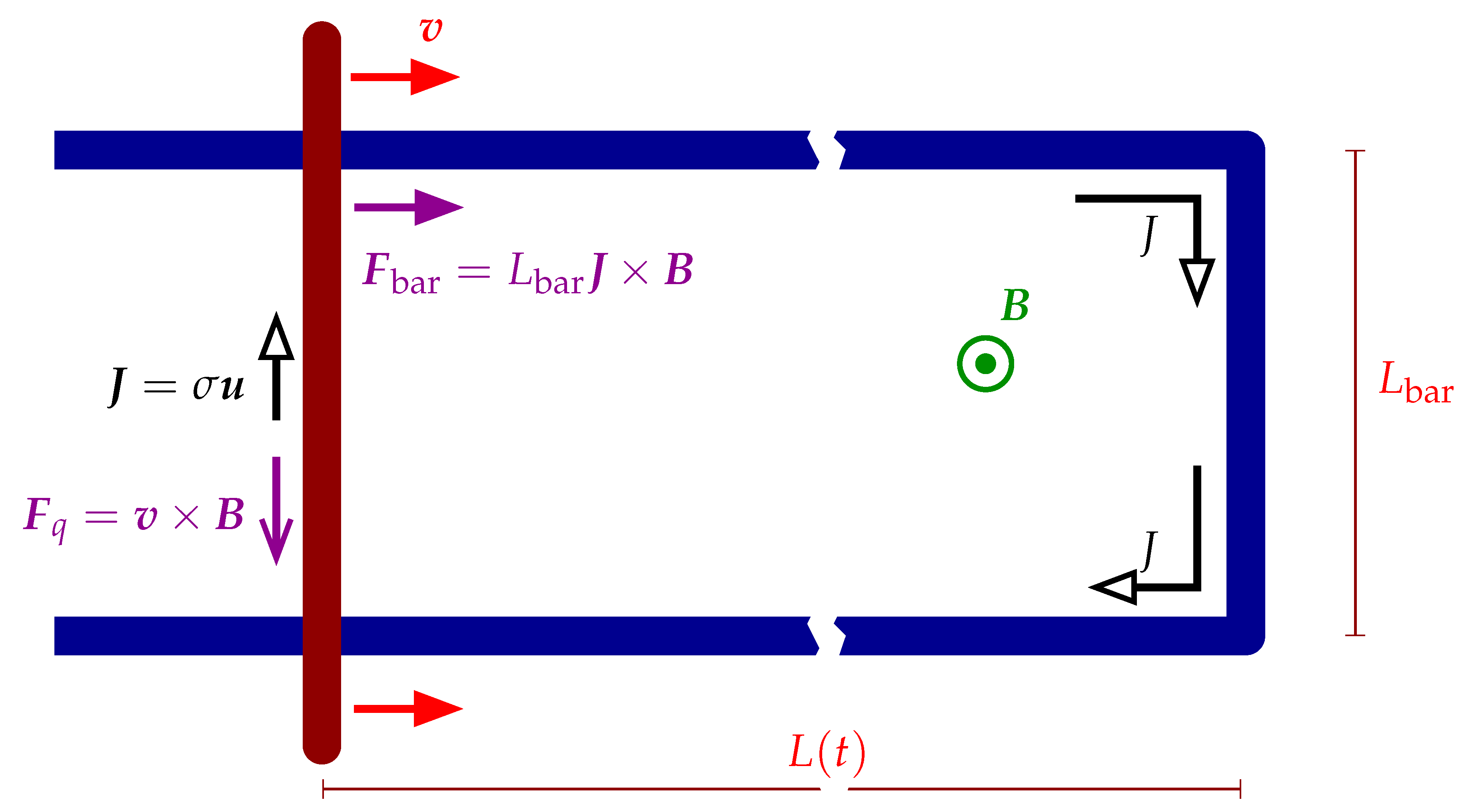
5.2. U-Shaped Bar and Moving Rod
Let us now try to make more progress by treating a specific situation instead of abstract constructions. Consider the standard undergraduate style system of a long rectangular conducting U-shape in a constant magnetic field, with a conducting bar closing a current loop, as depicted in Figure 5. The bar then is said to slide along the arms of the U, thus changing the area enclosed by the loop, hence changing the enclosed flux. We might then straightforwardly apply Faraday’s Law from the l.h.s. of Equation (1), and use the rate of change of flux to calculate an EMF, and then (if we want to) an induced current associated with that EMF.
However, given our decision to insist on there being a particular causal interpretation, and because Faraday’s Law does not comply with that interpretation, we must therefore choose a different mathematical model. Since without assuming spatial gradients of the field, which are not a necessary feature of our example, we cannot use the Ampere-based expression in Equation (19), we will start with the force law. However, using the Lorentz Force Law Equation (21) means that we can see immediately that there are two forces on charges relevant here:
First, there is the the magnetic force on the charges in the bar, due to the motion of the bar in the magnetic field. This force is oriented along the bar, modifying the charge velocity in the bar, and then by extension in the entire loop.
Second, there is a magnetic force on the charges in the bar, due to the along-bar motion of those charges in the magnetic field. This force pushes the charges perpendicular to the bar, which can be related to the Hall effect. Here we assume that this Hall effect rapidly polarizes the bar, on a timescale much faster than other processes, so that the net effect shows only in a residual slowing force on the bar itself.
This means that we can use the force law to calculate (a) how the current J in the loop responds to the velocity of the bar, and (b) how the motion of the bar responds to the current J in the loop. These will naturally be dynamic equations with an explicit causality.
Here we take the wire U to be fixed and rigid, so that any forces on it due to current flow within it, and/or the presence of electromagnetic fields, are neglected. The wire U itself has arbitrarily long arms with a separation and base length of , each with a linear charge density . The bar has mass M and velocity , to give a momentum . It is mounted perpendicular to the wire U’s arms, a distance L from their base, and (also) has a charge density and length .
The current J consists of flow of charges with forward momentum . It has a total charge Q, but with only in the bar, which is the only part that gets pushed by the magnetic force. If the (effective) mass density of the charges [21] is , the velocity of the charges along the bar is , and their speed is where . The corners of the U and the contacts between the U and the bar are assumed to divert (e.g., perhaps by elastic reflection) the charges around the loop (i.e., into their new direction), so that is only either forward (clockwise on Figure 5) or backward (anticlockwise) around the loop; the charge density of the current is also assumed to be fixed [22].
The total force on the bar is only due to the magnetic force, which needs to be summed over the length . Note that the field inside the loop is not important here, what counts is its strength at each point in the bar, at the instant the total force is integrated. The force density on each element of the bar is
so that in total we get
The total force on the current is not only the magnetic force, which needs to be summed over the bar’s length , but also includes a linear resistive term , where and r is proportional to resistance per unit length. Note that (again) the field inside the loop is not important here, what counts is its strength along the bar at its current location. Since the speed of the bar along the wires is , the force density on each element of the current is
so that in total, we have
These are two linear coupled differential equations, and can be combined most easily by taking the time derivative of the equation, and substituting one into the other. Simplifying the equations by not displaying the explicit time dependences of and , we get
where
Note that we cannot directly replace with current J in the differential equations, since they are related via the total conductor length . Further, the driving term dependent on is proportional to , which has its own dynamics: if the magnetic field is changing in time, it is not sufficient to try to solve only Equation (37), we also need to consider Equation (30).
Since there are some complicated interdependences contained within this result, we now consider some instructive special cases.
5.2.1. Constant Magnetic Field
Consider the case where the magnetic field is a constant over all time as well as space, so that , i.e., the third r.h.s. term of Equation (37) vanishes. Here, the bar, after being given an initial push, will oscillate forwards and backwards according to the frequency parameter , but with the amplitude of those oscillations dying away with a rate given by .
We can also see that for small variations in and , the frequency parameter will be effectively constant, and so become a true frequency of oscillation. In this regime, we can straightforwardly substitute with the current , and get
This would result in damped sinusoidal variations in current, and hence related oscillations in the speed of the bar; since the acceleration of the bar can be related to the current by Equation (30).
5.2.2. Time Varying Magnetic Field
Equation (37) has retained the possibility for a time-dependent . We can see that the change in the field acts to accelerate the current, but in manner dependent on (i.e., the bar velocity). So the current still wants to oscillate, albeit in a way unlikely to be a simple sinusoid, with the field changes acting as a driving term.
5.2.3. Electro-Motive Force
We can now consider what Equation (37) tells us about the EMF induced in the loop; since what we are doing is based on the Lorentz force law, we use EMF rather than the usual Faraday Law . Since is the work per unit charge, or the line (loop) integral of the force, and force is just the change in the momentum, we have that . This means that for small changes in , we can almost reuse Equation (37) directly—we just apply another time derivative and substitute for , to get
The equation might at a first glance appear to show time-like changes in the magnetic field causing alterations in the EMF. Of course, since it contains more model dependent detail, some differences with standard Faraday’s Law in Equation (2) or the alternate Ampere-derived one in Equation (19) are to be expected.
The difficulty now is that the right hand side, as a direct result of the conversion from to now has a second order time derivative acting on B, just as does the left hand side acting on . Since they have equal orders of time derivative, they share the same causal status—combined together correctly they could be interpreted as being the effect of the other terms in Equation (40), i.e., the cause-like terms and , as well as ones involving v.
This means that Equation (40) does not have the causal interpretation we were searching for, e.g., such as where first-order time-like changes in the magnetic field caused second-order alterations in the EMF.
5.3. Discussion
Here we have seen that for both our force law based calculations, i.e., the very simple one and the more realistic system, both fail to supply us with a result where properties of the magnetic field can be said to cause changes in the EMF. Nevertheless, the causal attributions like that which we aimed for can still be made by not referring to the EMF, but instead using statements like (changes in) magnetic field properties induce currents.
6. Conclusions
In this paper we have tried to search for a version or rederivation of Faraday’s Law whose mathematical form mimics the causal interpretation we would like to have, namely changes in magnetic flux through a loop induce changes in the EMF around that loop. However, the usual mathematical form of Faraday’s Law is incompatible with this desire, and only allows us to say that EMF causes changes in flux.
To address this apparent deficiency, we derived a Faraday-like law based on the Maxwell Ampere curl equation, which indeed allowed us to talk of induced changes in the EMF, but these were instead caused by spatial gradients in the magnetic flux, which is not quite what we had hoped. This led us to try an alternative approach based on the Lorentz force law, whose microscopic foundations showed promise in that properties of the magnetic field indeed induced (caused) changes in current, both in an abstract and a more realistic setting. However, when the mathematical model was converted to refer instead to induced changes in an EMF-like quantity , we found that the model became incompatible with the desired causal interpretation, emphasizing that it is an insistence on using EMF which introduces the difficulty.
In summary, our investigation has shown that one should be careful when making causal interpretations of magnetic induction processes, and be wary of depending on hidden or implicit assumptions that can lead to misleading conclusions. First, one should clearly distinguish between interpretations relevant to an experiment, and those relevant to a mathematical model; a distinction that is vital in the case of Faraday’s Law. Second, since the closest we can get to a “changes in magnetic flux induces EMF” is based on the Maxwell Ampere equation and not Maxwell Faraday, we need to be careful when deciding on causal interpretations of empirical laws derived from or compatible with experiment.
Funding
I am grateful for the support provided by STFC (the Cockcroft Institute ST/G008248/1 and ST/P002056/1) and EPSRC (the Alpha-X project EP/N028694/1).
Acknowledgments
I would also like to acknowledge the hospitality of Imperial College London, many interesting discussions with Jonathan Gratus and Martin W. McCall, and all the others who have made helpful suggestions.
Conflicts of Interest
The author declares no conflict of interest.
References and Notes
- Bleaney, B.I.; Bleaney, B. Electricity and Magnetism, 2nd ed.; Clarendon Press: Oxford, UK, 1965. [Google Scholar]
- Bohren, C.F. What did Kramers and Kronig do and how did they do it? Eur. J. Phys. 2010, 31, 573. [Google Scholar] [CrossRef]
- Landau, L.D.; Lifshitz, E.M. Electrodynamics of Continuous Media; Pergamon: Oxford, UK; New York, NY, USA, 1984. [Google Scholar]
- Lucarini, V.; Saarinen, J.J.; Peiponen, K.E.; Vartiainen, E.M. Kramers-Kronig Relations in Optical Materials Research; Springer: Berlin/Heidelberg, Germany, 2005; Volume 110. [Google Scholar] [CrossRef] [Green Version]
- Kinsler, P. How to be causal: Time, spacetime, and spectra. Eur. J. Phys. 2011, 32, 1687. [Google Scholar] [CrossRef] [Green Version]
- Corduneanu, C. Functional Equations with Causal Operators; Taylor and Francis: London, UK; New York, NY, USA, 2002. [Google Scholar]
- Corduneanu, C. Existence of Solutions for Neutral Functional Differential Equations with Causal Operators. J. Differ. Equ. 2000, 168, 93–101. [Google Scholar] [CrossRef] [Green Version]
- Kinsler, P. How to be causal: Time, spacetime, and spectra. arXiv 2011, arXiv:1106.1792. [Google Scholar] There are additional appendicies in this e-print update comprared to [5].
- Kinsler, P. Time and space, frequency and wavevector: Or, what I talk about when I talk about propagation. arXiv 2014, arXiv:1408.0128. [Google Scholar]
- Kinsler, P. Uni-directional optical pulses, temporal propagation, and spatial and temporal dispersion. J. Opt. 2018, 20, 025502. [Google Scholar] [CrossRef] [Green Version]
- Rideout, D.P.; Sorkin, R.D. A Classical Sequential Growth Dynamics for Causal Sets. Phys. Rev. D 2000, 61, 024002. [Google Scholar] [CrossRef] [Green Version]
- Jefimenko, O. Presenting electromagnetic theory in accordance with the principle of causality. Eur. J. Phys. 2004, 25, 287–296. [Google Scholar] [CrossRef]
- Hill, S.E. Rephrasing Faraday’s Law. Phys. Teacher 2010, 48, 410–412. [Google Scholar] [CrossRef]
- Savage, C.M. Causality in classical electrodynamics. Phys. Teacher 2012, 50, 226. [Google Scholar] [CrossRef] [Green Version]
- Boyer, T.H. Faraday induction and the current carriers in a circuit. Am. J. Phys. 2015, 83, 263–271. [Google Scholar] [CrossRef] [Green Version]
- Thide, B. Electromagnetic Field Theory; Upsilon Books: Uppsala, Sweden, 2004. [Google Scholar]
- Jackson, J.D. Classical Electrodynamics, 3rd ed.; Wiley: Hoboken, NJ, USA, 1999. [Google Scholar]
- Reitz, J.R.; Milford, F.J.; Christy, R.W. Foundations of Electromagnetic Theory, 3rd ed.; Addison-Wesley: Reading, MA, USA, 1980. [Google Scholar]
- When looking up the definition of “induce” we see that it is in essence the same as “causes”. Some instances of the various phrasings of “cause”, “induce”, and “associated with” from the literature are discussed in the appendix of the preprint version of this paper at arxiv:1705.0840.
- Kumar, V. Electromagnetic response of a metal: A comparative analysis of the ‘free charge model’ and the ‘bound charge model’. Eur. J. Phys. 2017, 38, 045203. [Google Scholar] [CrossRef]
- Attempting to describe accurately how the charges respond as a group is difficult and complicated. One must somehow average over the many distinct microscopic influences on each charge: not only from its local environment in the conductor and any externally applied fields, but also the many interactions between it and the other charges [15,24,25] must be considered. Then we must combine all these into a net effect on the charges as a group. Here we simply reduce the combined effect of all such complications down into an effective mass density for the charges.
- A further detail, neglected here, is that each movement of the bar either orphans or inherits some extra charges due to the change in side-wide length.
- Kinsler, P. Active drains and causality. Phys. Rev. A 2010, 82, 055804. [Google Scholar] [CrossRef] [Green Version]
- Darwin, C.G. Inertia of electrons in metals. Proc. R. Soc. A 1936, 154, 61–66. [Google Scholar] [CrossRef] [Green Version]
- Essen, H. From least action in electrodynamics to magnetomechanical energy—A review. Eur. J. Phys. 2009, 30, 515–539. [Google Scholar] [CrossRef]
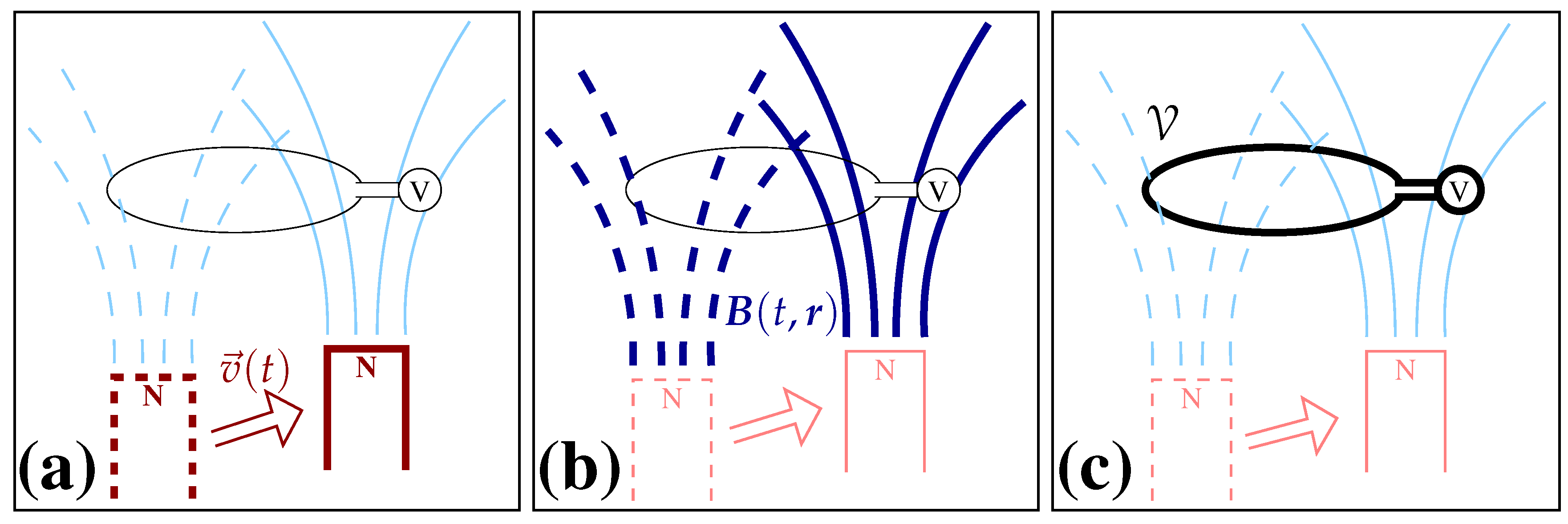
Figure 1.
An experiment: (a) a magnet (its north pole marked “N”) with velocity passes near a wire loop with a voltmeter ⓥ, so that (b) its magnetic field moves also, leading to (c) an EMF appearing around the loop. Although going from (a) to (b) is simple to model, being just a translation of the magnetic field of the magnet, there is much microscopic detail in (c), where those fields interact with the charges in the loop, inducing and altering currents, until the eventual effect on the EMF.

Figure 2.
Diagram showing the configuration and fields used for the induction equation based—as usual—on the Maxwell–Faraday equation in fields and . The loop that allows us to decide on the integration contour C is shown in light blue, and the surface of integration S is its cross-sectional disc.
Figure 2.
Diagram showing the configuration and fields used for the induction equation based—as usual—on the Maxwell–Faraday equation in fields and . The loop that allows us to decide on the integration contour C is shown in light blue, and the surface of integration S is its cross-sectional disc.
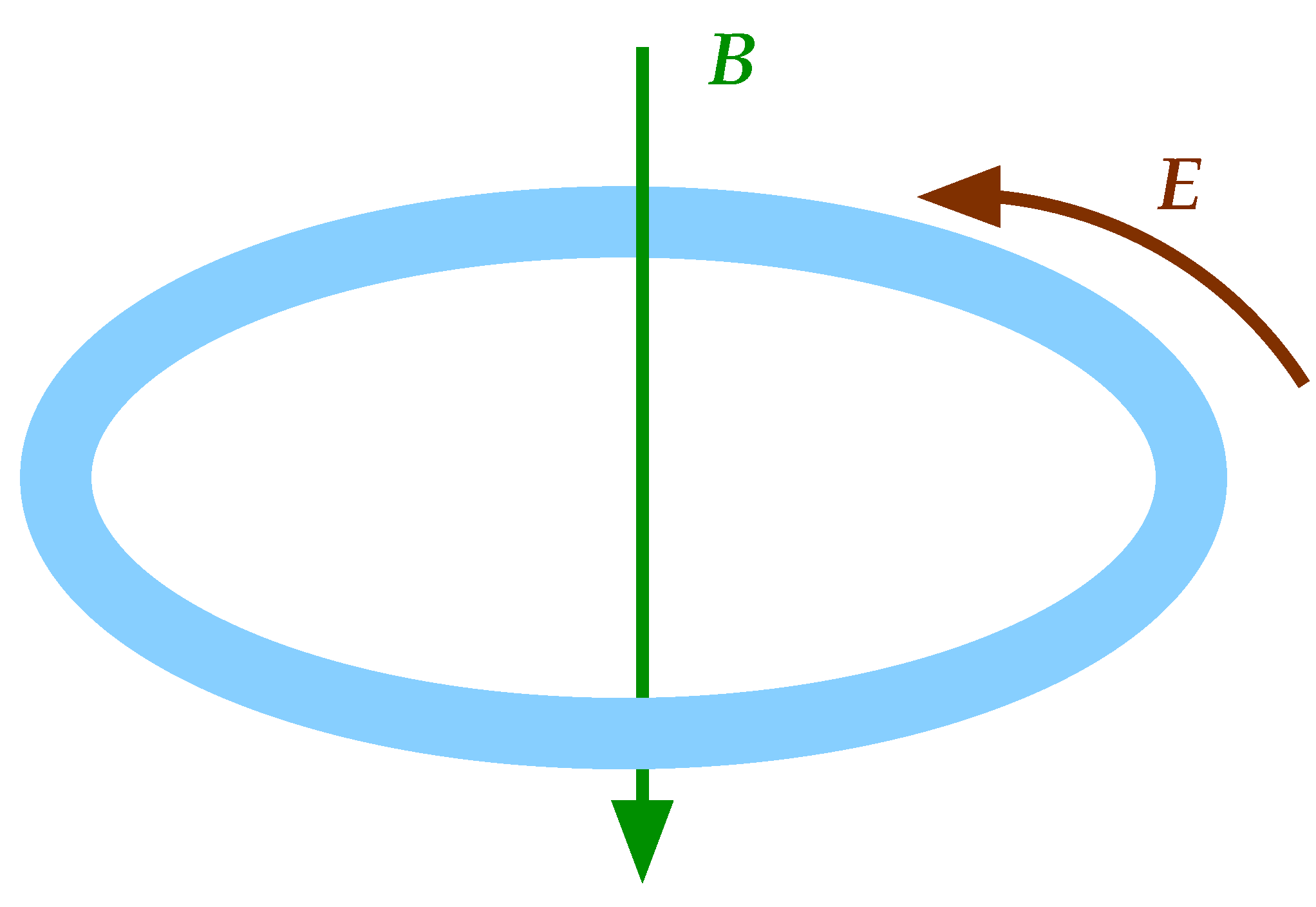
Figure 3.
Diagram showing the configuration and fields used for the induction equation based on the Maxwell–Ampere equation in fields and . The loop that allows us to decide on the integration contour C is shown in light blue, and the surface of integration S is its cross-sectional disc.
Figure 3.
Diagram showing the configuration and fields used for the induction equation based on the Maxwell–Ampere equation in fields and . The loop that allows us to decide on the integration contour C is shown in light blue, and the surface of integration S is its cross-sectional disc.
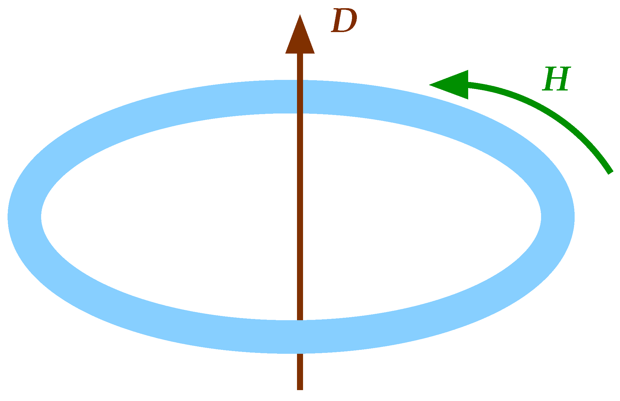
Figure 4.
The magnetic field and loop (integration contour) orientations used in reducing Equation (26) to Equation (27). The loop in the plane moves with speed v in the x direction through a z-directed magnetic field whose strength varies only with x (i.e., ).
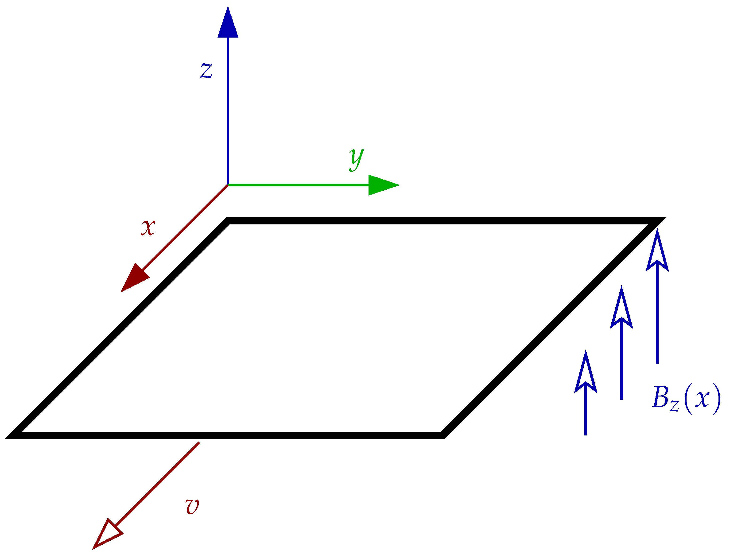
Figure 5.
Diagram showing the U-shaped bar in dark blue, and the moving rod in dark red. Black arrows indicate the current J, and red arrows show the (positive) motion of the moving bar. Magenta arrows indicate the two forces: one on the bar, as caused by the effect of the (its) current travelling through the magnetic field; and the other on the charges in the bar (and hence on the current), caused by the motion of the bar through the magnetic field. Along the bar, it is useful to express the current J as a vector (), to help with calculating the direction of .
© 2020 by the author. Licensee MDPI, Basel, Switzerland. This article is an open access article distributed under the terms and conditions of the Creative Commons Attribution (CC BY) license (http://creativecommons.org/licenses/by/4.0/).
Share and Cite
MDPI and ACS Style
Kinsler, P. Faraday’s Law and Magnetic Induction: Cause and Effect, Experiment and Theory. Physics 2020, 2, 150-163. https://doi.org/10.3390/physics2020009
AMA Style
Kinsler P. Faraday’s Law and Magnetic Induction: Cause and Effect, Experiment and Theory. Physics. 2020; 2(2):150-163. https://doi.org/10.3390/physics2020009
Chicago/Turabian StyleKinsler, Paul. 2020. "Faraday’s Law and Magnetic Induction: Cause and Effect, Experiment and Theory" Physics 2, no. 2: 150-163. https://doi.org/10.3390/physics2020009