An Expectation–Maximization-Based IVA Algorithm for Speech Source Separation Using Student’s t Mixture Model Based Source Priors


1
Department of Informatics, King’s College London, London WC2B 4BG, UK
2
Department of Engineering, University of Leicester, Leicester LE1 7RH, UK
*
Author to whom correspondence should be addressed.
Acoustics 2019, 1(1), 117-136; https://doi.org/10.3390/acoustics1010009
Submission received: 23 November 2018
/
Revised: 21 December 2018
/
Accepted: 29 December 2018
/
Published: 10 January 2019
(This article belongs to the Special Issue Room Acoustics)
Abstract
:The performance of the independent vector analysis (IVA) algorithm depends on the choice of the source prior to better model the speech signals as it employs a multivariate source prior to retain the dependency between frequency bins of each source. Identical source priors are frequently used for the IVA methods; however, different speech sources will generally have different statistical properties. In this work, instead of identical source priors, a novel Student’s t mixture model based source prior is introduced for the IVA algorithm that can adapt to the statistical properties of different speech sources and thereby enhance the separation performance of the IVA algorithm. The unknown parameters of the source prior and unmixing matrices are estimated together by deriving an efficient expectation maximization (EM) algorithm. Useful improvement in the separation performance in different realistic scenarios is confirmed by experimental studies on real datasets.
1. Introduction
The process of automated separation of acoustic sources from measured mixtures is known as acoustic blind source separation (BSS) [1]. The typical application of blind source separation is to handle the cocktail party problem, which is the process of focusing on one particular acoustic source of interest in the presence of multiple sound sources [2,3,4]. Human beings can easily pay attention to one of the speakers in the presence of multiple active speakers; however, it is much more difficult to replicate the same ability in machines [5]. In the past few decades, much research has been conducted to study different aspects of the cocktail party problem. This research includes the study of the geometry of the microphone array [6], room impulse response identification [7], localisation of speech sources [8] and statistical estimation of speech sources [9]. Independent component analysis (ICA) is one of the fundamental techniques to solve the cocktail party problem. The ICA algorithm was proposed by Herault and Jutten [10,11]; however, it has limitations such as permutation and scaling problems [12,13,14]. The IVA algorithm is an extension of the ICA algorithm which was proposed to theoretically mitigate the permutation problem of the ICA method that is inherent to most of the BSS algorithms [15].
The IVA algorithm is based on a dependency model which retains inter-frequency dependencies within each source vector. The dependent sources are arranged together as a multivariate variable in the frequency domain components of a signal. When the IVA algorithm is compared with the ICA algorithm, the inter-frequency dependencies within each source depend on the modified prior of the source signal. In the ICA algorithm, independence for each frequency component is measured separately at each frequency bin. On the other hand, the IVA method formulates the problem by considering that the dependencies exist between frequency bins rather than assuming the independence for frequency bins. The source priors in conventional algorithms were defined as independent priors; however, within the IVA algorithm each source prior is defined as a multivariate super-Gaussian distribution. Therefore, the cost function for the IVA algorithm is minimised only when the dependency between the source vectors is removed but the dependency among the components of each vector is preserved [16]. Hence it measures the dependence across the whole multivariate source and it can retain the higher order inter-frequency dependencies and structure of frequency components. Therefore, choosing an appropriate dependency model for the IVA algorithm is crucial to the performance of the algorithm.
Statistically the process of human speech production is highly complex [4,17,18] and the human speech signal is non-stationary in nature. Furthermore, the human speech signal is difficult to model with one fixed model as there can be wide variations in human speech, i.e., properties of natural speech vary from person-to-person and depend on which language is being spoken as the pronunciation rates and phonemes can be completely different in different parts of the world. Moreover, recorded speech is dependent on variations in room acoustics and microphone characteristics, e.g., different rooms will have different reverberation effects and different microphones will have variable frequency responses [3]. All of these factors can change the observed human speech signal and thereby different speech signals generally have different statistical properties. Hence, it is important that the BSS algorithms adapt their statistical structure according to the characteristics of the observed speech signals.
The IVA algorithm preserves the inter-frequency dependency between the individual sources in the frequency domain. The IVA method uses the score function and its form is crucial to the performance of the IVA algorithm. The score function is derived by statistical modelling of the speech sources by selecting an appropriate source prior. Speech signals are often characterized with single distribution statistical models that does not change according to the nature of speech signals. In the original IVA [15] method all the speech sources were modelled by identical multivariate Laplacian distributions. Different sources can have different statistical properties and modelling all the sources with identical distribution may not be the most appropriate solution. As a result a novel potential approach is to adopt the Student’s t mixture model (SMM) as a source prior for the IVA algorithm, instead of the conventional identical multivariate distributions. The probability density function of the Student’s t mixture model (SMM) has heavier tails as compared to other super Gaussian models and therefore it can model outliers in the data [19,20,21]. As human speech is highly random, the spread of samples can be very wide, and the SMMs, due to its heavier tails, can generally model high amplitude information in human speech more accurately [22].
The new framework of the expectation-maximization (EM) algorithm is implemented efficiently for the proposed IVA algorithm to estimate the unmixing matrices. The EM algorithm is a two step iterative approach which efficiently estimates the unknown parameters of the source prior and unmixing matrices. The EM method overcomes non-analytically solvable problems and it has been commonly used in the field of statistics, signal processing and machine learning [23]. By using SMMs as the source prior and implementing the new framework of EM, the proposed IVA algorithm shows performance improvement when compared with previous approaches [15,21,24,25]. To the best of our knowledge, there are no other studies that are using SMMs as source prior for the IVA algorithm to achieve robust and improved performance for different speech mixtures in realistic scenarios.
The rest of the paper is organized as follows. We begin by explaining the related work in the next section. We begin by explaining the IVA algorithm and related work in Section 2. It is followed by detailed description of the proposed EM framework for the IVA algorithm with SMMs as source priors in Section 3. Experimental results in realistic scenarios and comparisons between the proposed approach and other state-of-the-art methods are presented in Section 4. Finally, some concluding remarks are included in Section 5.
2. Related Work
In order to implement the IVA algorithm for the convolutive BSS, the short time Fourier transfer (STFT) is used to convert the problem from the time domain to the frequency domain as it eases the computational complexity of the time domain method. The basic noise free BSS model for the IVA method in the frequency domain can be defined as follows:
where is a mixing matrix of dimensions . The index k represents the k-th frequency of this multivariate method. In order to separate the source signals from the observed mixtures, an unmixing matrix must be estimated to retrieve the estimate of the original sources, as
where is the estimated source signal, , is the unmixing matrix of dimensions . In this paper, focus is on the exactly determined case, so the number of sources is considered equal to the number of microphones, i.e., .
In order to model the independence between sources, the IVA method uses the Kullback-Leibler divergence. So a cost function can be derived as follows [15]:
where represents the matrix determinant and shows the expectation operator. All the sources in the cost function of the IVA algorithm are multivariate and the cost function will be minimised when different vector sources become independent of each other and the dependency within each source vector is retained. Hence this cost function can be used to eliminate the dependency between the vector sources and preserve the frequency dependency within each vector source.
Previously, in the IVA method, speech signals have been modelled with various superGaussian distributions, e.g., the Laplacian distribution [15] or generalized Gaussian distribution [26] but speech signals can have very high and low amplitudes and other superGaussian distributions may not be able to accurately model the high amplitudes in the speech signals [27,28,29]. Therefore, new source priors are still needed to improve the performance of the IVA algorithm.
3. Proposed Method
In order to model the speech signals with low and high amplitude, the Student’s t distribution is adopted as a source prior for the IVA method. The multivariate Student’s t distribution is given as: A K-dimensional random separated source vector can have a K-variate t distribution with degree of freedom , precision matrix and mean , if its joint pdf is given by [27]:
In the joint pdf of the Student’s t distribution, the leptokurtic nature and the variance of distribution can be adjusted by tuning the degrees of freedom parameter [30]. When the parameter is set to a lower value, the tails of the distribution becomes heavier and if is increased to infinity, the Student’s t distribution tends to a Gaussian distribution [19,20]. Since different sources can have different statistical properties, so instead of using identical Student’s t source prior for all sources, the Student’s t mixture model (SMM) is adopted as a source prior in this work. By adopting the SMM as a source prior, different speech sources can be modelled with different SMMs thereby enabling the IVA method to adapt to the statistical properties of different types of signals. Assuming the sources are statistically independent, for a 2 × 2 case, an SMM can be represented as:
where is the weight of the mixture component of the SMM source prior for source i and K represents the total number of frequency bins in the multivariate model. The precision matrix is defined as the inverse of the covariance matrix and its -th element satisfies . With appropriate normalisation and zero mean assumption, the Student’s t distribution can be written as:
When the vector of frequency components is considered from the same source i, the interdependency between these frequency components is preserved whereas the vectors that originate from different sources are independent of each other. Therefore, by adopting this inter-frequency dependency model, the IVA method prevents the permutation problem that is inherent to most BSS methods [4].
In the IVA algorithm, the scaling of mixture signal and mixing matrix cannot be determined by the separated source signals , therefore observations are prewhitened. Because of the prewhitening process, both the mixing matrix and the unmixing matrix are unitary matrices. In this work, the 2 × 2 case has been considered, so the Cayley Klein parameterizations [31] for the unitary matrix are as follows:
In the next section, the maximum likelihood estimate is derived for the IVA algorithm.
3.1. Maximum Likelihood Estimation of SMM
The maximum likelihood estimate is a well-known method that is usually used to estimate the mixture parameters. Based on the maximum likelihood method, the mixture parameters can be effectively estimated iteratively via the EM algorithm [23]. The log likelihood function for t components mixture of Student’s t distributions is considered and it is given as:
where consists of the model parameters for the log likelihood function; is the PDF of the observed source mixture signals which is an SMM as it is generated by the SMM source priors. The denotes the unmixing matrix, represents the precision matrix and is the collective mixture index of the SMMs for the source prior. In the maximum likelihood estimation, the best fitting model helps to estimate parameters that can maximize the log-likelihood function, which is usually performed by using the EM algorithm [23]. Therefore, the model parameters set can be estimated by training the SMM and maximizing the log likelihood function by using the EM algorithm. The detailed method for estimating the model parameters by the EM algorithm is explained in the next section.
3.2. The Expectation-Maximization Algorithm
The EM algorithm is suitable in finding latent parameters in probabilistic models by using an iterative optimization technique [23]. The EM algorithm is implemented by introducing discrete random variables which are dependent on the observations and the model parameter set . The log likelihood function with these variables is given by
and can be used to optimise the model parameters. In the case of an increasing log likelihood function, a lower bound is formed on the increasing log likelihood for the observations . So the new parameters that increase the log likelihood function of the complete data with respect to current parameters, can be found. Hence there is an increase in the expected log likelihood of the complete data with respect to current parameters and it is produced by the updated parameters. Therefore, an auxiliary function can be used to represent the expected log likelihood function. There will be a definite increase in the log likelihood function when the auxiliary function is optimised but it does not necessarily yield a maximum likelihood solution [23]. Therefore, it is important to iteratively calculate and maximize the auxiliary function until convergence. Hence a local approximation is made which is the lower bound to the objective function. By using the Jensen’s inequality [32], the lower bound for the log likelihood function in Equation (11) can be calculated as follows:
The EM algorithm will run until convergence and it will iteratively maximize in two steps. The first step is the expectation step in which the posterior probability of the hidden variable is calculated over and in the second step, the is updated.
3.3. The Expectation Step
In the expectation step, is fixed and is maximised over . In order to maximise , the derivative of the log-likelihood equation with respect to is calculated as follows:
In order to maximize for fixed , Equation (13) is equalised to zero and with appropriate normalization,
Now by using ,
and the precision matrix for the 2 × 2 case can be written as:
As is a unitary matrix, therefore and from Equation (10), the function can be defined as:
By using Equation (14), function can be rewritten as , therefore:
Next, the maximization step is considered.
3.4. The Maximization Step
In the maximization step (M-step) the parameters can be estimated by maximising the cost function. In this step, each parameter is estimated separately. In the first step, the maximisation of over the unitary constraint is considered. In order to maximize the , the precision matrix for the 2 × 2 case can take the following form:
When Equation (15) is rearranged and is replaced in the log likelihood Equation (12), it will take the following form:
By using the log approximation , where a is a small value, the above mentioned equation can take the following form, wherein equality is assumed for convenience.
By further manipulating the above mentioned equation, details of which are given in Appendix A, the parameters of the unmixing matrix can be calculated as follows:
Since the unmixing matrix , it can be estimated by using the above mentioned analytical solution. It is an efficient method to estimate the unmixing matrix as the above mentioned method avoids the matrix calculations.
The model parameters are estimated by maximizing the log likelihood function. Therefore, now will be maximized over and and they are given as follows.
where denotes the element of the matrix. So over using the above mentioned solution.
Now, maximisation of over is performed and it is given as:
Hence the weighting parameter can be calculated by using the above mentioned equation. Detailed derivation for maximization of is included in Appendix A.
It can be seen that the EM algorithm effectively estimates all the model parameters . The E-step updates the , while the M-step effectively estimates the model parameters. In the EM algorithm the degrees of freedom parameter is fixed in advance for all the sources, then the M-step exists in the closed form (Algorithm 1). The value for the degrees of freedom can be estimated empirically for different source signals. The complete EM framework for the SMIVA algorithm is summarized as follows.
| Algorithm 1 EM algorithm for Student’s t Mixtures |
Require: Given a Student’s t mixture model, the aim is to maximize the log likelihood function with respect to the parameters .
|
The separation performance of this EM framework for the SMIVA method will be evaluated in the next section.
4. Experimentations and Results
In this section, the separation performance of the SMIVA algorithm will be tested in three different experimental setups. Firstly, the new framework for the IVA algorithm is tested in a simulated environment and then in order to evaluate the performance in real scenarios, it is tested with real room impulse responses (RIRs), which can depict the performance of the proposed method in changing realistic settings. The results from all three sets of experiments for the proposed algorithm will be compared with the original IVA algorithm with different source priors.
4.1. Case I: Simulations with the Image Method
Firstly, the proposed method will be tested with RIRs that were generated by using the image method. The speech signals were selected randomly from the whole of the TIMIT dataset [33] and the length of speech signals was approximately 4 s. A 2 × 2 case was considered and the room has the = 200 ms and it provides a good setup for comparing the separation performance of different algorithms. The positions of microphones in the room were set to [3.44, 2.50, 1.50] and [3.48, 2.50, 1.50] with azimuth angles of and , respectively with reference to the normal of the microphone position. The STFT length is 1024 and sampling frequency is 8 kHz. The separation performance of the algorithm was evaluated with the objective measure of SDR [34]. The common parameters used in these experiments are summarised in Table 1.
The speech signals were convolved into mixtures in the above mentioned room settings. These speech mixtures were then separated by using the proposed SMIVA method and the separation results for different mixtures were compared with the separation performance of the original IVA method with the original super Gaussian source prior [15] and also with the IVA method with Student’s t source prior [21] and the results are shown in Table 2 and all the values shown for SDR are in dB. For each mixture SDR performance shown in the Table 2 is the average of two speech signals. It is evident from the Table 2 that when the SMM is adopted as a source prior, the average SDR improvement is approximately 1.1 dB for all the mixtures as compared to the original super Gaussian source prior for the IVA method. It is evident from Table 2 that the SMM source prior based SMIVA algorithm enhances the separation performance of the IVA method with a single distribution source prior, such as the Student’s t distribution and also the original super Gaussian.
For the derivation purposes, the unmixing matrix W is assumed to be unity in this study. In order to measure the effect of this assumption on the performance of the SMIVA algorithm, its separation performance is compared with the algorithms that do not place the same restriction on the solution such as [36,37]. Since the latent variables are modelled with a single distribution in these methods, the SMIVA algorithm is also adjusted to a uni-model case by using a single Student’s t distribution. For the sake of consistency in results, same experimental settings are used as in the previous case and the SDR measure is used to estimate the separation performance of the algorithms and the results are shown in Figure 1. It is clear from results that the SMIVA algorithm with the assumptions placed on the solution space still consistently perform better than the algorithms that does not have the same assumptions on the solution space. These results shows the significance of the modelling of the high and low amplitude information within the speech signals by using the Student’s t distribution.
In order to further investigate the separation performance of the SMIVA algorithm, its separation results are compared with the other mixture model source prior such as Gaussian mixture model [24] in the next section with real RIRs.
4.2. Case II: Simulations with Real RIRs
In the second set of experiments, the proposed SMIVA algorithm is tested with real RIRs. These real RIRs are obtained from [38] and these are recorded in different rooms with different acoustic properties. Three different room types (A, B, D) have been used with of 320 ms, 470 ms and 890 ms, respectively. By using these RIRs the proposed method can be tested with the range of reverberation time. Therefore, these simulations show the performance of the proposed algorithm in real life scenarios as the can vary drastically in realistic environments [39]. Different source location azimuth angles are available, which range from to , relative to the second source.
Firstly, the proposed algorithm is tested in Room A, which is a typical medium sized office and it has the of 320 ms, which is relatively small for a medium size office. In the experiments two speech signals are randomly chosen from the whole of the TIMIT dataset and the source location azimuth angles are set to be from to with a step of . The mixed sources are separated by using the proposed SMIVA method and the separation performance in terms of SDR is compared with the IVA using the identical Student’s t source prior [21] and also with the original super Gaussian source prior based IVA method [15]. The separation performance for both methods is evaluated for six different angles varying from to with a step of . At all the angles separation performance is averaged over six different speech mixture and the results are presented in Figure 2.
It is evident from Figure 2 that when proposed algorithm is used to separate the mixtures and the performance is compared with identical distribution source prior for the IVA, it consistently has a better separation performance at all the selected azimuths angles and approximately 1 dB of improvement in SDR values is recorded at all the angles as compared to the original IVA method [15].
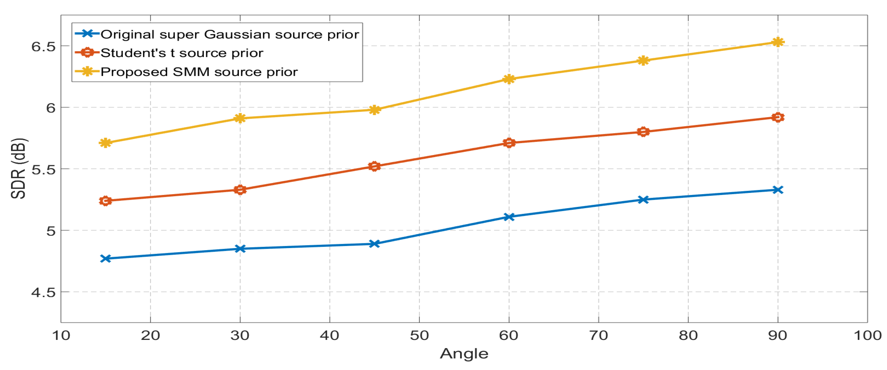
The same set of experiments are then repeated for room-B, which evaluate the performance of the algorithms in more challenging and realistic scenarios as it is a medium size classroom with of 470 ms. The separation performance in terms of SDR of both methods for six different azimuth angles is showed in Figure 3. It is evident from the result that the EM framework SMIVA performs better than the identical source priors for the original IVA method at all separation angles in ths reverberant real room environment.
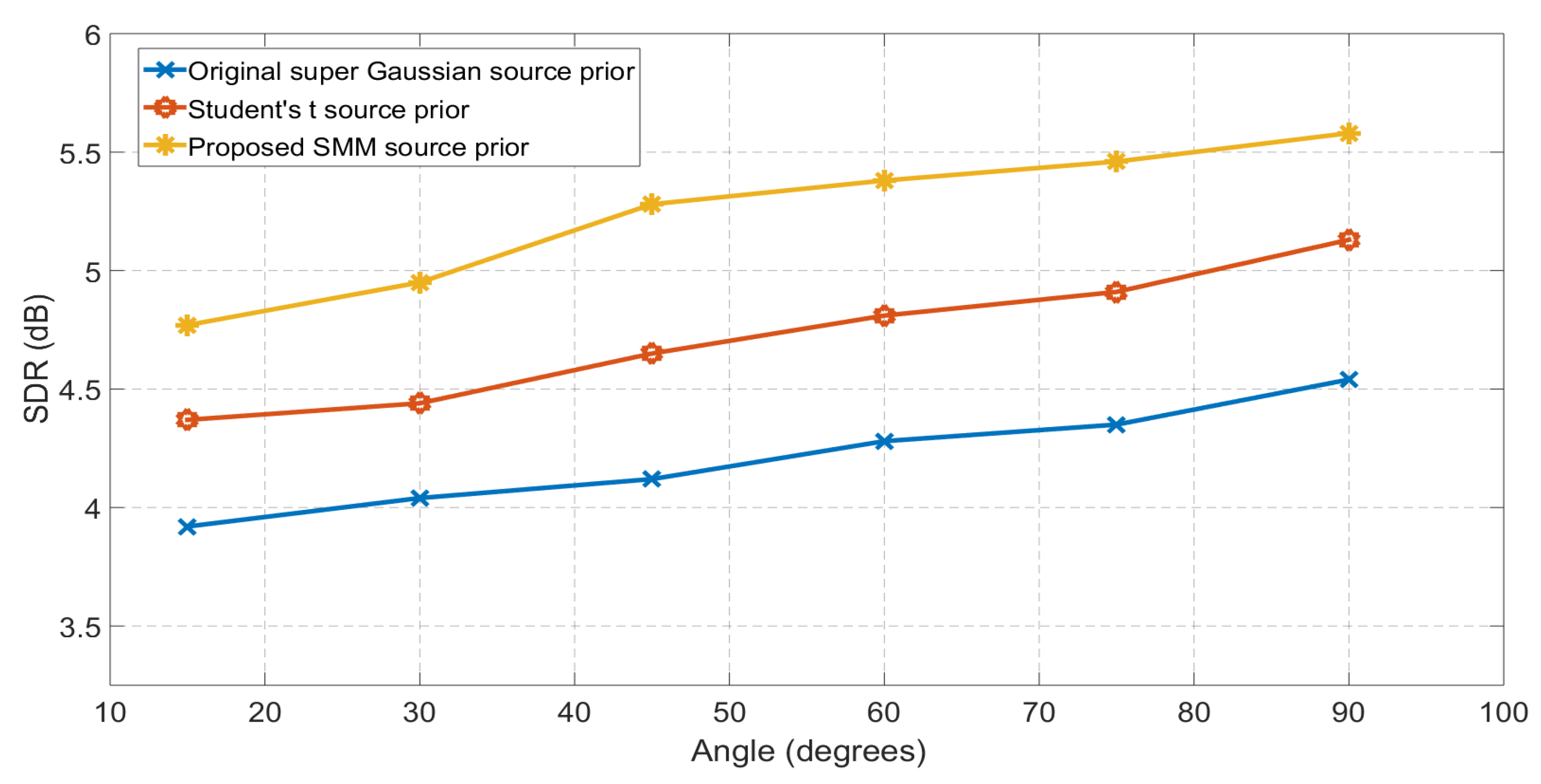
Finally, the separation performance of the proposed EM framework for the IVA method is evaluated in a highly reverberant realistic environment that can depict the performance of the algorithm in the real life scenarios. For the highly reverberant environment, Room D was used which is a medium size seminar and presentation hall with a very high ceiling. The for this seminar hall is 890 ms, which is high reverberation time and therefore it provides a good insight into the algorithm’s performance in an extremely difficult real life situations. The experimental setup in this highly reverberant room D is similar to the previous two rooms. The mixtures were separated with the IVA method with different source priors and the separation performance in terms of SDR for all methods is shown in Figure 4 for all six angles varying from to . The SDR values in room D is lower in comparison with the SDR values for Room-A and Room-B, it is mainly because the for Room D is really high as compared to the other two rooms. Also, it is evident from the Figure 4 that even in this highly reverberant environment the IVA method with SMM source prior performs better than the identical distribution source priors for the original IVA with Student’s t source prior and improves the average SDR performance of the original IVA method by approximately 0.8 dB.
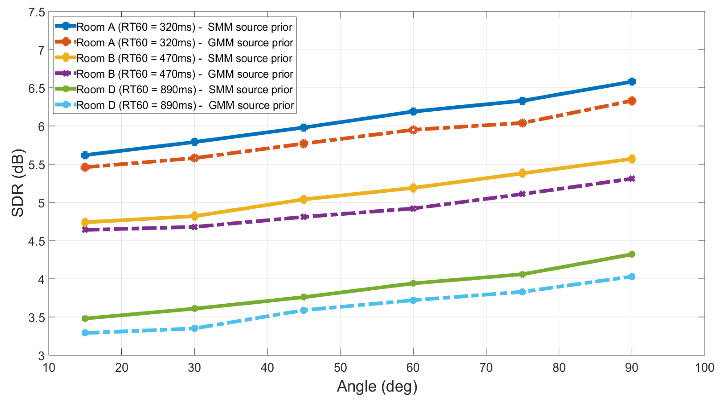
The separation performance of the proposed EM framework for the IVA algorithm with SMMs as a source prior is also compared with the IVA algorithm with a Gaussian mixture model (GMM) as a source prior [24]. Since the mixture model is adapted as a source prior for the IVA algorithm, the comparison with other mixture models, i.e., GMM can provide better understanding of the separation performance of the proposed source prior. In this set of experiments, a mixture of two Gaussians is adapted as source prior for the IVA algorithm and the rest of the parameters are adjusted similar to the SMIVA algorithm and simulations are performed in the real room settings. For the experimental setup, same settings for Room A, B and D are used as in the previous case and speech signals are randomly chosen from TIMT dataset. Initially, experiments are performed in room A, which has of 320 ms and it is repeated for six different source location varying from to . Similarly, the same experimental setup is used for room B with of 470 ms and for room D with of 890 ms. In all the rooms mixtures are separated by using the EM framework IVA with both SMM and GMM source priors and the separation performance in terms of SDR is compared with the proposed method at six different source azimuth angles varying from to . All the SDR values at all the angles are the average of separation performance of six different mixtures. The separation performance of both methods for all three rooms with the range of is shown is Figure 5 and it is evident that the IVA method with SMM as a source prior has better separation performance than IVA with GMM as a source prior.
4.3. Case III: Simulations with Binaural Room Impulse Responses
The proposed algorithm is further tested with binaural room impulse response (BRIRs) obtained from [40]. These BRIRs are recorded in a real classroom which roughly has dimensions of 5 × 9 × 3.5 m . The six source location azimuths relative to the right of listener were used for the experimentation. Also the distance between the source were changed three times and 1 m). The measurements for the BRIRs are taken at four different listener locations (back, ear, corner and center) and the distance between the floor and ears was approximately 1.50 m. In these experiments only center location is used and the at the center location for the classroom was 565 ms. All the measurements are repeated on three different occasions by taking down the equipment and reassembling it which improves the reliability of the measurements. Therefore, these BRIRs have been used in the experiments as they are reliable and also provide accurate estimate of the separation performance of the BSS algorithms in highly reverberant room environments. A summary of different parameters used in this set of experiments is given in Table 3.
The 2 × 2 case was considered for the experiments and speech signals were randomly chosen from the whole TIMIT dataset and mixtures were created by using BRIRs. The length of the speech signals was approximately four seconds. The speech signals were then separated from the mixtures by using the proposed EM framework for the IVA algorithm with SMM as source prior. The separation performance of the proposed algorithm is compared with the separation performance of the IVA with GMM as source prior for the IVA algorithm. It provides a good estimate for the separation performance of the proposed algorithm and source prior as comparison is drawn with mixture model source priors. The separation performance in terms of SDR is shown in Table 4 for the six different source location . All the experiments are repeated three times and at each source location six different speech mixtures are separated. In order to improve the reliability of results, all the SDR values are the average of separation performance of the algorithms over eighteen different speech mixture.
From Table 4 it is evident that when the SMM is used as a source prior for the IVA algorithm it performs better as compared with the GMM as a source prior. Since speech signals are highly non-stationary in nature and there can be many useful samples in outliers which might not be properly modelled with the Gaussian mixtures but Student’s t mixtures because of its heavy tails can model the outlier information and therefore enhance the separation results of the IVA method. When the SMM is adopted as a source prior for the IVA method, at all the source location azimuths it improves the average separation performance for the IVA method by more than for all the angles as shown in Table 4.
Furthermore, the separation performance is evaluated with the subjective measure of PESQ [41]. This subjective measure compares the original signals and separated signals and gives a score from 0 to 4.5, 0 for the poor separation performance and 4.5 being the excellent separation performance. This measure therefore provides a good estimate about the similarity between the original and separated sources. So the speech mixtures made with BRIRs are separated with the proposed SMM source prior for the EM framework IVA and also with the GMM source prior IVA and the PESQ score is calculated for both the methods. The PESQ score for the IVA method with both source priors is shown in Table 5 and the IVA method with SMM source prior consistently has the better PESQ score as compared with the GMM source prior for the IVA algorithm. The PESQ score was generally low in this experiment because of difficult room environment. However, it is evident from the table that when SMM is adapted as a source prior, it improves the separation performance for the IVA method.
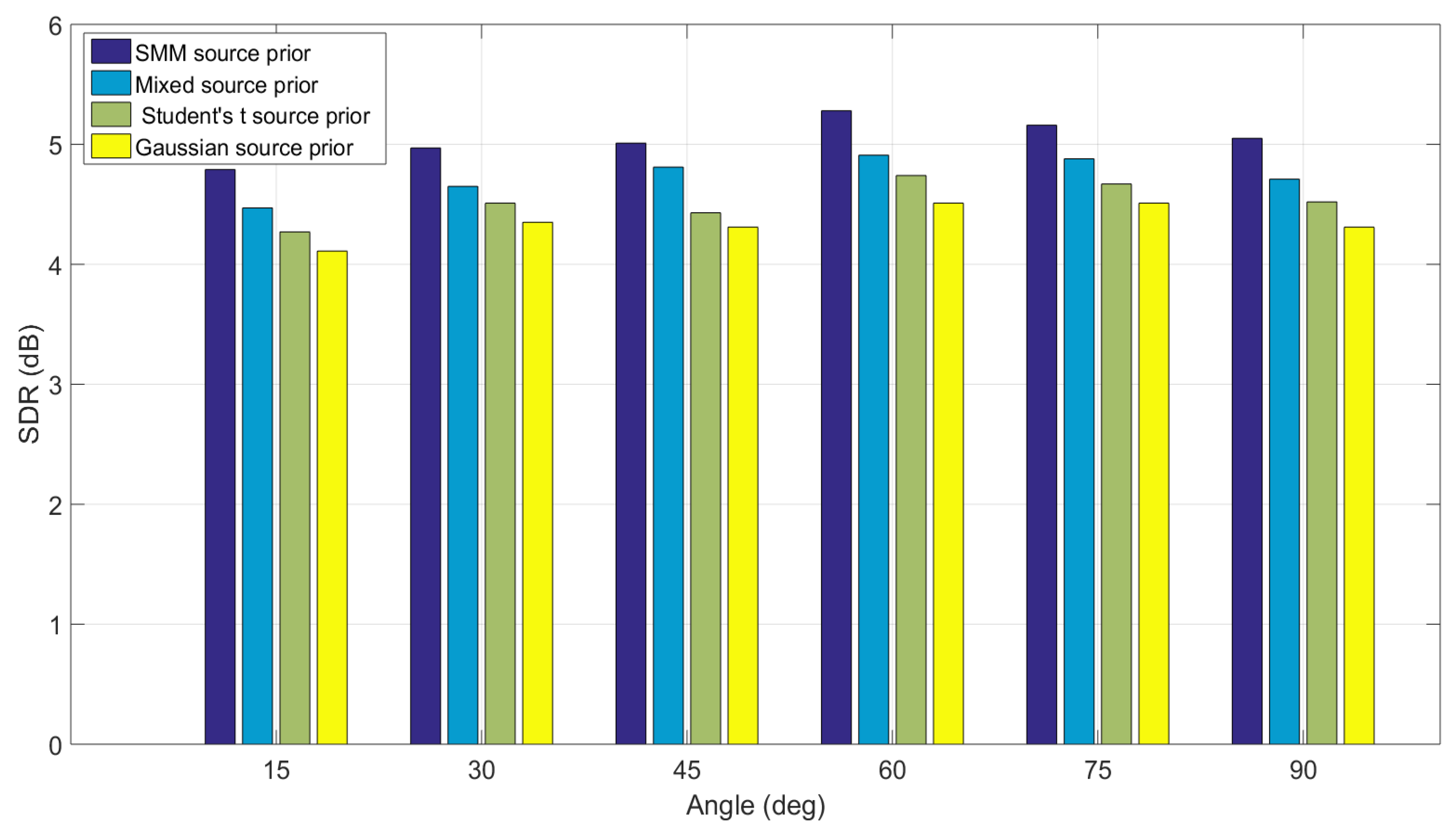
Finally, the separation performance of the proposed EM framework for the IVA method with SMM as source prior is compared with the original IVA with identical source priors. BRIRs with of 565 ms are used to evaluate the algorithms in highly reverberant environment that can depict the performance of the algorithms in the realistic scenarios. The Same experimental settings are used as in the first experiments and the source location is varied six times from . All the measurements are repeated three times and six different speech mixtures are separated at each angle by using IVA method with SMM as source prior and the results are compared with the separation performance of IVA method with multivariate Student’s t distribution as source prior, the IVA method with original multivariate super Gaussian source prior and also with IVA method with the mixed Student’s t and original super Gaussian source prior. This provides an overall comparison of the separation performance of different source prior and the framework for the IVA method. The results in terms of SDR (dB) for six different source location are shown in Figure 6.
It is evident from Figure 6 that the mixture model source prior performs better than the identical distribution source prior at all the source locations. Since different speech sources can have different statistical properties and the mixture model such as SMM source prior can model different sources with different Student’s t distribution in the mixture model while identical source prior model all the sources with the identical distribution and therefore their separation performance suffers as compared to the mixture model source priors.
5. Conclusions
This work presented the EM framework for the IVA method that uses the mixture of Student’s t distribution as a source prior in order to better model the different statistical properties in different speech sources. The mixture of Student’s t distribution source prior made use of the heavy tails nature of the Student’s t distribution to effectively model the high amplitude information in the speech signal. The complete EM framework was derived efficiently to estimate the model parameters for the IVA method. The separation performance for the proposed method was tested with image room impulse method and it confirms the advantage of using the proposed framework for the IVA method as it shows the SDR improvement of approximately 1 dB as compared to the original IVA method. Further experiments were conducted in real room environments with different reverberation times. In varying reverberant environment, new SMIVA consistently performed better as compared to other source priors and provides average SDR improvement of 0.8 dB. In order to further test the new SMIVA algorithm, it was tested with BRIRs and the SMM source prior improves the separation performance as compared to the GMM source prior and in all case, improvement of more than in SDR performance was recorded. This improvement in the separation performance can be further verified and used by implementing the algorithm in real time practical scenarios, which remain the topic for future work in this study. All the simulations performed with different real room environments confirmed that the proposed EM framework for the IVA algorithm that make use of the SMM source prior improves the separation performance even in highly reverberant real room environments.
Author Contributions
W.R.—Methodology, investigation, experimentation, validation, writing, reviewing and editing; J.C.—Methodology, reviewing, supervision and resources; A.I.S.—writing, reviewing and editing.
Funding
This research received no external funding.
Acknowledgments
The authors would like to thank the anonymous reviewers for their valuable comments and suggestions to improve the quality of the paper.
Conflicts of Interest
The authors declare no conflict of interest.
Appendix A. The EM framework for SMIVA
The log likelihood function for t components mixture of Student’s t distributions is given in Equation (10) as:
Expectation step is already derived and is given by Equation (18):
Next the maximization step is derived in detailed. The MATLAB implementation for the SMIVA algorithm is available online (https://github.com/wr27/The-IVA-algorithm-with-SMM-source-prior).
The maximization step (M-step) the parameters are estimated by maximising the cost function. Firstly, the maximisation of over the unitary constraint is considered. The precision matrix can be written in the following form
Now Equation (15) can be rearranged as:
Now by replacing the value of the precision in the above equation
The above equation can be rewritten by replacing the value of from the Equation (A3) as follows:
After appropriate manipulation and ignoring the constant terms, Equation (A6) takes the following form:
Now by replacing the value of and for the 2 × 2 case:
After the matrix multiplication, the previous equation takes the following form:
Now by taking the derivative of above mentioned equation with respect to and equalising to zero.
Likewise, taking the derivative with respect to and equating it to zero
Assuming and by Equations (A10) and (A11):
where vector is the eigenvector of with the smaller eigenvalue. This can be found by replacing in Equation (A7) and taking trace of the equation:
where denotes the trace of the matrix. Whereas the eigenvectors associated with the smaller eigenvalues will give the higher value of the cost function. Therefore, is the eigenvector of with the smaller eigenvalue. In order to calculate the eigenvalues associated with the for the 2 × 2 case, can be written as:
where , are real and , because is Hermitian. Eigenvalues in this case can be calculated as:
Since the above equation is a quadratic equation, therefore the quadratic formula can be used to find the eigenvalues which are , so the smaller eigenvalue can be written as:
Hence, by using this analytical approach, computational complexity can be reduced as this approach avoids any matrix calculation.
Again, by using the log approximation , where a is a small value, the above equation can take the following form, wherein equality is consider for convenience.
By replacing the value of in the Equation (A20) and by taking the derivative with respect to yields
After appropriate manipulation, coefficient of precision matrix are estimated as follows.
where denotes the element of the matrix. So over using the above mentioned solution.
Now in the final step, maximisation of over is performed. The lower bound of the log likelihood equation is:
If can take s possible states, has to satisfy . So does not have s degrees of freedom instead it has free parameters. So, the Lagrange multiplier is used in this case. Therefore, the cost function can be described as:
Now taking the derivative of the above mentioned equation with respect to and equating it to zero yields:
Now and , therefore the above equation can be rewritten as:
Hence the weighting parameter can be calculated by using the above mentioned equation. It can be seen that the EM algorithm effectively estimates all the model parameters . The E-step updates the , while the M-step effectively estimates the model parameters. The above mentioned E-step and M-step will keep iterating until convergence criteria is fulfilled.
References
- Haykin, S. Unsupervised Adaptive Filtering (Volume I: Blind Source Separation); Wiley: Hoboken, NJ, USA, 2000. [Google Scholar]
- Cherry, C. Some experiments on the recognition of speech, with one and with two ears. J. Acoust. Soc. Am. 1953, 25, 975–979. [Google Scholar] [CrossRef]
- Haykin, S.; Chen, Z. The cocktail party problem. Neural Comput. 2005, 17, 1875–1902. [Google Scholar] [CrossRef] [PubMed]
- Cichocki, A.; Amari, S. Adaptive Blind Signal and Image Processing; John Wiley: Hoboken, NJ, USA, 2002. [Google Scholar]
- McDermott, J.H. The cocktail party problem. Curr. Biol. 2009, 19, R1024–R1027. [Google Scholar] [CrossRef] [PubMed] [Green Version]
- Wang, D.; Brown, G. Fundamentals of computational auditory scene analysis. In Computational Auditory Scene Analysis: Principles, Algorithms and Applications; John Wiley and Sons: Hoboken, NJ, USA, 2006; pp. 1–44. [Google Scholar]
- Adali, T.; Anderson, M.; Geng-Shen, F. Diversity in independent component and vector analyses: Identiability, algorithms, and applications in medical imaging. IEEE Signal Process. Mag. 2014, 31, 18–33. [Google Scholar] [CrossRef]
- Parra, L.; Alvino, C. Geometric source separation: merging convolutive source separation with geometric beamforming. IEEE Trans. Speech Audio Process. 2002, 10, 352–362. [Google Scholar] [CrossRef]
- Pedersen, M.S.; Larsen, J.U.; Kjems, U.; Parra, L.C. A survey of convolutive blind source separation methods. Springer Handb. Speech Process. Speech Commun. 2007, 8, 1–34. [Google Scholar]
- Jutten, C.; Herault, J. Blind Seperation of sources, part I: An adaptive algorithm based on neuromimetic architecture. Signal Process. 1991, 24, 1–10. [Google Scholar] [CrossRef]
- Jutten, C.; Comon, P. Handbook of Blind Source Separation: Independent Component Analysis and Applications; Academic Press: Cambridge, MA, USA, 2010. [Google Scholar]
- Lee, T.W. Independent Component Analysis: Theory and Applications; Kluwer Academic: Norwell, MA, USA, 2000. [Google Scholar]
- Hyvrinen, A. Fast and robust fixed-point algorithms for independent component analysis. IEEE Trans. Neural Netw. 1999, 10, 626–634. [Google Scholar] [CrossRef] [Green Version]
- Parra, L.; Spence, C. Convolutive blind separation of non-stationary sources. IEEE Trans. Speech Audio Process. 2000, 8, 320–327. [Google Scholar] [CrossRef]
- Kim, T.; Attias, H.; Lee, S.; Lee, T. Blind source separation exploiting higher-order frequency dependencies. IEEE Trans. Audio Speech Lang. Process. 2007, 15, 70–79. [Google Scholar] [CrossRef]
- Kim, T.; Lee, I.; Lee, T.W. Independent vector analysis: Definition and algorithms. In Proceedings of the Fortieth Asilomar Conference on Signals, Systems and Computers, Pacific Grove, CA, USA, 29 October–1 November 2006. [Google Scholar]
- Simonyan, K.; Ackermann, H.; Chang, E.F.; Greenlee, J.D. New developments in understanding the complexity of human speech production. J. Neurosci. 2016, 36, 11440–11448. [Google Scholar] [CrossRef] [PubMed]
- Cooke, M.; Ellis, D. The auditory orgnization of speech and other sources in listeners and computational models. Speech Commun. 2001, 35, 141–177. [Google Scholar] [CrossRef]
- Sun, Y.; Rafique, W.; Chambers, J.A.; Naqvi, S.M. Underdetermined source separation using time-frequency masks and an adaptive combined Gaussian-Student’s t probabilistic model. In Proceedings of the 2017 IEEE ICASSP, New Orleans, LA, USA, 5–9 March 2017; pp. 4187–4191. [Google Scholar]
- Sundar, H.; Seelamantula, C.S.; Sreenivas, T. A mixture model approach for formant tracking and the robustness of Student’s t distribution. IEEE Trans. Audio Speech Lang. Process. 2012, 20, 2626–2636. [Google Scholar] [CrossRef]
- Rafique, W.; Naqvi, S.M.; Jackson, P.J.B.; Chambers, J.A. IVA algorithms using a multivariate Student’s t source prior for speech source separation in real room environments. In Proceedings of the IEEE ICASSP, South Brisbane, QLD, Australia, 19–24 April 2015; pp. 474–478. [Google Scholar]
- Rafique, W. Enhanced Independent Vector Analysis for Speech Separation in Room Environments. Ph.D. Thesis, Newcastle University, Newcastle upon Tyne, UK, 2017. [Google Scholar]
- Bishop, C.M. Pattern Recognition and Machine Learning; Springer-Verlag: Secaucus, NJ, USA, 2006. [Google Scholar]
- Hao, J.; Lee, I.; Lee, T.W.; Sejnowski, T.J. Independent Vector Analysis for Source Separation Using a Mixture of Gaussians Prior. Neural Comput. 2010, 22, 1646–1673. [Google Scholar] [CrossRef] [Green Version]
- Rafique, W.; Erateb, S.; Naqvi, S.M.; Dlay, S.S.; Chambers, J.A. Independent vector analysis for source separation using an energy driven mixed Student’s t and super Gaussian source prior. In Proceedings of the 2016 24th European Signal Processing Conference (EUSIPCO), Budapest, Hungary, 29 August–2 September 2016. [Google Scholar]
- Liang, Y. Enhanced Independent Vector Analysis for Audio Separation in a Room Environment. Ph.D. Thesis, Loughborough University, Loughborough, UK, 2013. [Google Scholar]
- Peel, D.; McLachlan, G.J. Robust mixture modelling using the t distribution. Stat. Comput. 2000, 10, 339–348. [Google Scholar] [CrossRef]
- Rafique, W.; Naqvi, S.M.; Chambers, J.A. Speech source separation using the IVA algorithm with multivariate mixed super Gaussian Student’s t source prior in real room environment. In Proceedings of the IET Conference Proceedings, London, UK, 1–2 December 2015. [Google Scholar]
- Rafique, W.; Naqvi, S.M.; Chambers, J.A. Mixed source prior for the fast independent vector analysis algorithm. In Proceedings of the IEEE Sensor Array and Multichannel Signal Processing Workshop (SAM), Rio de Janeiro, Brazil, 10–13 July 2016; pp. 1–5. [Google Scholar]
- Aroudi, A.; Veisi, H.; Sameti, H.; Mafakheri, Z. Speech signal modeling using multivariate distributions. EURASIP J. Audio Speech Music Process. 2015, 2015, 35. [Google Scholar] [CrossRef]
- Bauchau, O.A.; Trainelli, L. The vectorial parametrization of rotation. J. Nonlinear Dyn. 2003, 32, 71–92. [Google Scholar] [CrossRef]
- Dragmor, S.S.; Goh, C.J. Some counterpart inequalities in for a functional associated with Jensen’s inequality. J. Inequal. Appl. 1997, 1, 311–325. [Google Scholar] [CrossRef]
- Garofolo, J.S.; Lamel, L.F.; Fisher, W.M.; Fiscus, J.G.; Pallett, D.S.; Dahlgren, N.L.; Zue, V. TIMIT Acoustic-Phonetic Continuous Speech Corpus; Linguistic Data Consortium: Philadelphia, PA, USA, 1993. [Google Scholar]
- Vincent, E.; Fevotte, C.; Gribonval, R. Performance measurement in blind audio source separation. IEEE Trans. Audio Speech Lang. Process. 2006, 14, 1462–1469. [Google Scholar] [CrossRef] [Green Version]
- Allen, J.B.; Berkley, D.A. Image method for efficiently simulating small-room acoustics. J. Acoust. Soc. Am. 1979, 65, 943–950. [Google Scholar] [CrossRef]
- Andreson, M.; Adali, T.; Li, X.L. Joint blind source separation with multivariate Gaussian model: Algorithms and performance analysis. IEEE Trans. Signal Process. 2012, 60, 1672–1682. [Google Scholar] [CrossRef]
- Boukouvalas, Z.; Fu, G.-S.; Adali, T. An efficient multivariate generalized Gaussian distribution estimator: Application to IVA. In Proceedings of the 2015 49th Annual Conference on Information Sciences and Systems (CISS), Baltimore, MD, USA, 18–20 March 2015. [Google Scholar]
- Hummersone, C. A Psychopsychoacoustic Engineering Approach to Machine Sound Source Separation in Reverberant Environments. Ph.D. Thesis, University of Surrey, Guildford, UK, 2011. [Google Scholar]
- ISO 3382-2: 2008. Acoustics. Measurements of Room Acoustics Parameters, Part 2; ISO: Geneva, Switzerland, 2008. [Google Scholar]
- Shinn-Cunningham, B.; Kopco, N.; Martin, T. Localizing nearby sound sources in a classroom: Binaural room impulse responses. J. Acoust. Soc. Am. 2005, 117, 3100–3115. [Google Scholar] [CrossRef]
- Hu, Y.; Loizou, P.C. Evaluation of Objective Quality Measures for Speech Enhancement. IEEE Trans. Audio Speech Lang. Process. 2008, 16, 229–238. [Google Scholar] [CrossRef]
Figure 1.
SDR (dB) values for algorithms without restriction on the solution space and SMIVA algorithm. The SMIVA algorithm shows better separation for all mixtures.
Figure 1.
SDR (dB) values for algorithms without restriction on the solution space and SMIVA algorithm. The SMIVA algorithm shows better separation for all mixtures.
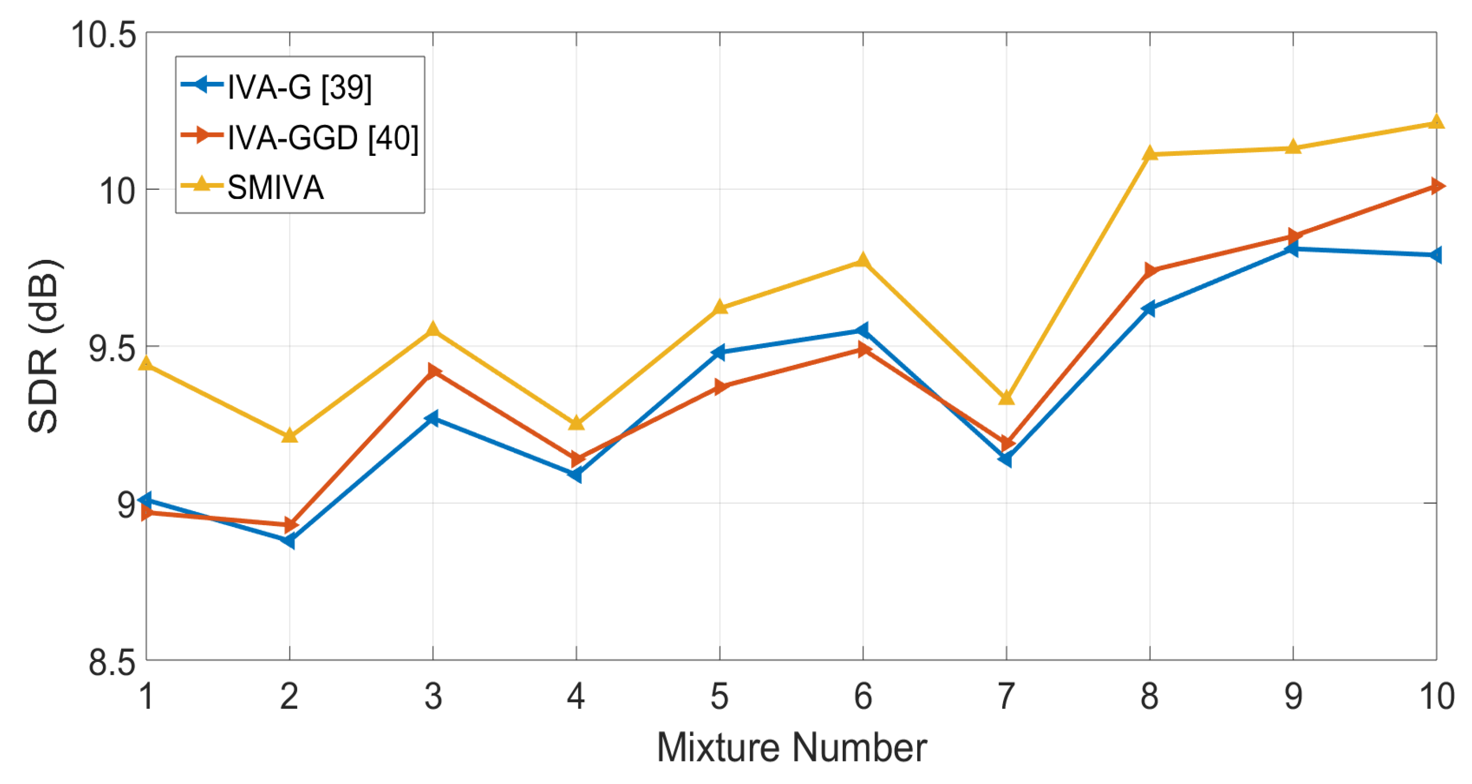
Figure 2.
Comparison between original IVA with original super Gaussian source prior, Student’s t source prior and EM framework IVA with SMM source prior for Room-A ( = 320 ms). The separation performance at each angle is averaged over six different speech mixtures. The proposed mixture model IVA performs better than a single Student’s t distribution at all the separation angles.

Figure 3.
Comparison between original IVA with Student’s t source prior and EM framework IVA with SMM source prior for Room-B ( = 470 ms). The separation performance at each angle is averaged over six different speech mixtures. The proposed mixture model IVA perform better than single Student’s t distribution at all the separation angles.

Figure 4.
Comparison between Original IVA with Student’s t source prior and EM framework IVA with SMM source prior for Room-D ( = 890 ms). The separation performance at each angle is averaged over six different speech mixtures. The proposed mixture model IVA performs better than single Student’s t distribution at all the separation angles.
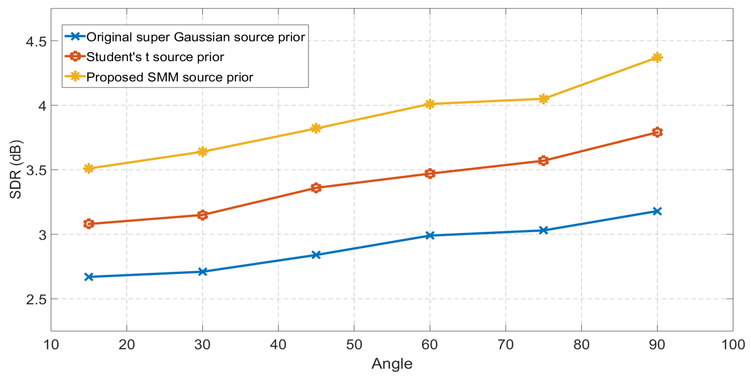
Figure 5.
Comparison between EM framework IVA with SMM and GMM source prior for three different rooms (Room-A, Room-B, Room-D). The separation performance at each angle is averaged over six different speech mixtures. The EM framework IVA algorithm with proposed SMM source prior performs better than GMM source prior at all the separation angles.

Figure 6.
Comparison between different source priors for the IVA algorithm for BRIRs ( = 565 ms). The separation performance at each angle is averaged over eighteen different speech mixtures. The IVA algorithm with proposed mixture model Student’s t source prior perform better at all the separation angles in comparison to identical source prior for all the sources.


Table 1.
Summary of parameters used in experiments.
| Sampling rate | 8 kHz |
| STFT frame length | 1024 |
| Reverberation time | 200 ms |
| Room dimensions | 7 m × 5 m × 3 m |
| Source signal duration | 4 s (TIMIT) |
| Room impulse responses | Image method |
| Objective measure | Signal to Distortion Ratio (SDR) |
Table 2.
SDR (dB) values for different source priors for the IVA method with an image room impulse response [35]. The SMM source prior shows improvement for all mixtures.
Table 2.
SDR (dB) values for different source priors for the IVA method with an image room impulse response [35]. The SMM source prior shows improvement for all mixtures.
| Original Super Gaussian | Student’s t Distribution | SMM Source Prior | |
|---|---|---|---|
| Set-1 | 9.09 | 9.84 | 10.27 |
| Set-2 | 8.98 | 9.72 | 10.24 |
| Set-3 | 9.26 | 10.11 | 10.87 |
| Set-4 | 9.02 | 9.95 | 10.49 |
| Set-5 | 9.53 | 10.21 | 10.62 |
| Set-6 | 9.51 | 10.14 | 10.74 |
| Set-7 | 8.91 | 9.67 | 10.09 |
| Set-8 | 9.86 | 10.48 | 11.05 |
| Set-9 | 9.94 | 10.66 | 11.24 |
| Set-10 | 10.02 | 10.56 | 11.01 |
Table 3.
Summary of parameters used in experiments.
| Sampling rate | 8 kHz |
| STFT frame length | 1024 |
| Velocity of sound | 343 m/s |
| Reverberation time | 565 ms (BRIRs) |
| Room dimensions | 9 m × 5 m × 3.5 m |
| Source signal duration | 3.5 s (TIMIT) |
Table 4.
Comparison between SMM source prior and GMM source prior for the EM framework IVA algorithm with BRIRs ( = 565 ms). The separation performance at each angle is averaged over eighteen different speech mixtures. The IVA algorithm with proposed mixture model Student’s t source prior perform significantly better at all the separation angles than the GMM source prior.
| GMM Source Prior | SMM Source Prior | Percentage Improvement | |
|---|---|---|---|
| Angle- | 4.51 | 4.82 | 6.87% |
| Angle- | 4.62 | 4.97 | 7.56% |
| Angle- | 4.77 | 5.09 | 6.70% |
| Angle- | 4.97 | 5.32 | 7.04% |
| Angle- | 4.91 | 5.28 | 7.73% |
| Angle- | 4.77 | 5.12 | 7.34% |
Table 5.
PESQ score for GMM and SMM source prior for the IVA algorithm.
| GMM Source Prior | SMM Source Prior | |
|---|---|---|
| Set-1 | 1.85 | 2.02 |
| Set-2 | 1.98 | 2.11 |
| Set-3 | 1.96 | 2.13 |
| Set-4 | 2.02 | 2.19 |
| Set-5 | 1.93 | 2.14 |
| Set-6 | 2.08 | 2.21 |
© 2019 by the authors. Licensee MDPI, Basel, Switzerland. This article is an open access article distributed under the terms and conditions of the Creative Commons Attribution (CC BY) license (http://creativecommons.org/licenses/by/4.0/).
Share and Cite
MDPI and ACS Style
Rafique, W.; Chambers, J.; Sunny, A.I. An Expectation–Maximization-Based IVA Algorithm for Speech Source Separation Using Student’s t Mixture Model Based Source Priors. Acoustics 2019, 1, 117-136. https://doi.org/10.3390/acoustics1010009
AMA Style
Rafique W, Chambers J, Sunny AI. An Expectation–Maximization-Based IVA Algorithm for Speech Source Separation Using Student’s t Mixture Model Based Source Priors. Acoustics. 2019; 1(1):117-136. https://doi.org/10.3390/acoustics1010009
Chicago/Turabian StyleRafique, Waqas, Jonathon Chambers, and Ali Imam Sunny. 2019. "An Expectation–Maximization-Based IVA Algorithm for Speech Source Separation Using Student’s t Mixture Model Based Source Priors" Acoustics 1, no. 1: 117-136. https://doi.org/10.3390/acoustics1010009