Mathematical Description of Rooting Profiles of Agricultural Crops and its Effect on Transpiration Prediction by a Hydrological Model

Abstract

The geometry of rooting systems is important for modeling water flows in the soil-plant-atmosphere continuum. Measured information about root density can be summarized in adjustable equations applied in hydrological models. We present such descriptive functions used to model root density distribution over depth and evaluate their quality of fit to measured crop root density profiles retrieved from the literature. An equation is presented to calculate the mean root half-distance as a function of depth from root length density profiles as used in single root models for water uptake. To assess the importance of the shape of the root length density profile in hydrological modeling, the sensitivity of actual transpiration predictions of a hydrological model to the shape of root length density profiles is analyzed using 38 years of meteorological data from Southeast Brazil. The cumulative root density distributions covering the most important agricultural crops (in terms of area) were found to be well described by the logistic function or the Gompertz function. Root length density distribution has a consistent effect on relative transpiration, hence on relative yield, but the common approach to predict transpiration reduction and irrigation requirement from soil water storage or average water content is shown to be only partially supported by simulation results.

1. Introduction

The quantitative description of the spatial distribution of the root system in the soil profile is an important topic for the modeling of water and solute uptake patterns by roots in the soil-plant-atmosphere continuum at several scales [1,2]. In land surface models, radiation balances, and to a lesser degree, precipitation patterns, appear to be sensitive to rooting distribution patterns [3,4,5]. Some research, such as [6], has attempted to present root profile parameters for specific vegetation types to be used in these models. At the field and plant scale, models describing the relation between yield and soil water content, and water content related variables such as irrigation amount, drainage, and groundwater level, have a long tradition in agriculture [7,8]. Detailed agro-hydrological simulations performed by robust process-based models, such as Hydrus [9] and SWAP [10], require root density distribution profiles. Moreover, the fact that root water uptake is closely related to biomass production [11] is at the core of ecological and agricultural analyses of water-limited growth and water use efficiency.

Equally important in modeling biomass production is quantifying nutrient uptake and its effect on crop yield. The relations between root density, root architecture, and nutrient uptake are frequent subjects of research [12,13,14,15,16,17,18,19,20]. Models for water and nutrient uptake have been formulated at two scales: the scale of the root system and the scale of a single root [16,21]. At both scales, also referred to as macroscopic and microscopic, respectively, root density is an important parameter. At the single root scale, a more detailed representation, root length density (root length per volume soil) determines the average distance between roots modeled as parallel cylinders [22,23]. At the scale of the root system, an often-used hypothesis is to assume that root water uptake is linearly proportional to root length density [21,24,25]. Detailed root water uptake reduction functions, which usually describe compensation mechanisms, are dependent on the absolute values of root length density distribution over the soil profile. This will determine the rhizosphere radius and the distribution of root water uptake. In this sense, crops with low root density will need higher hydraulic gradients between roots and the surrounding bulk soil in order to attend the atmospheric water demand. On the other hand, crops with higher root density can maintain the root water potential closer to that of the bulk soil and then postponing the drought stress [23]. Those mechanisms are highly dependent on the soil hydraulic properties and for this reason a well-represented root distribution allows accounting for the hydraulic ability of each soil layer in supplying water to plants.

Robust modeling frameworks have been developed to describe the complete three-dimensional (3-D) architecture and the dynamics of root growth and distribution [2,14,26] together with associated water extraction patterns [27]. In addition to the 3-D modeling tools, one-dimensional (1-D) models with root length density (RLD) representation are well known for allowing good predictions of macroscopic root water uptake [24,28,29]. Reviews of root density profiles as determined in field experiments have been presented for several agricultural crops and water/irrigation regimes, e.g., [30,31,32,33], and for different ecological biomes [34,35,36].

At the field scale, rooting patterns are generally heterogeneous. In the case of agricultural crops, they are influenced by local conditions such as tillage, fertilization, aeration, and nutrient and water availability, as well as other soil factors such as chemistry and texture. In this context, although hardly ever present in dynamic water balance or crop growth models, the strong feedback between root growth and soil water deficit [37,38,39] is important to consider. At a global scale and for natural vegetation, results presented by [40] support a relation between deep roots, soil type, and climate.

We aim to present and mathematically analyze some descriptive functions used to model root density distribution over depth. We then test the quality of fit of the equations by fitting them to experimentally established crop root density profiles, following the setup of the database compiled by [35]. In addition, we provide an approximation of the mean root half-distance for use in upscaled single root models for nutrient and water uptake. In order to assess the importance of the shape of the root length density profile in agro-hydrological simulation, the sensitivity of actual transpiration predicted by a hydrological model was analyzed as a function of the shape of root length density profiles.

2. Materials and Methods

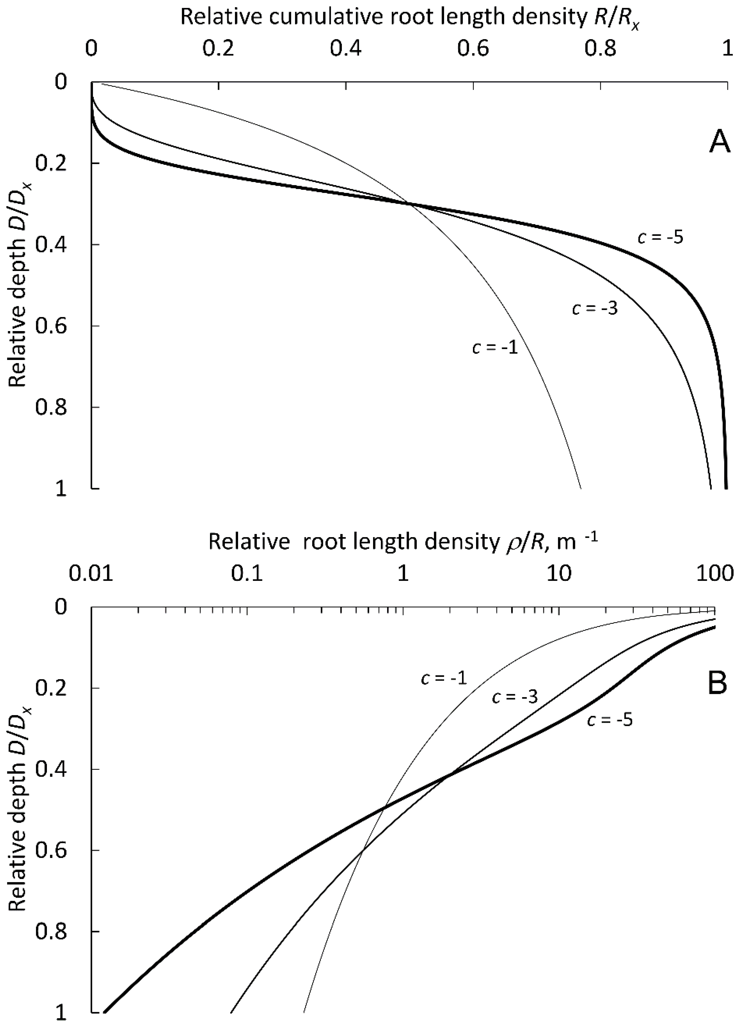
2.1. Mathematical Description of Root Density Profiles

The cumulative root density R (m⁻¹) describes the integral of root length density ρ (m m⁻³ = m⁻²) over profile depth D (m) as a function of depth z (m), at a given time:

$$R={\displaystyle \underset{0}{\overset{D}{\int }}\mathsf{\rho }dz}$$

(1)

Equation (1) implies that R = 0 at the soil surface. Here R is expressed in length units, but reported measurements may sometimes be in mass or in counts. If these measures are linearly proportional to root length and the proportionality constant is not a function of depth, descriptions of root density profiles using different measurement procedures differ by a proportionality constant only, and the shape of the curve is identical. For instance, a linear relation between root mass density and root length density was presented for potato [41]. The shape of root profiles was compared using different measurement methods and the assumption that the shape does not change for different measurement procedures holds for different biomes [35]. This assumption allows the pooling of data determined by different measurement methods to describe the shape of root density curves. Therefore, in the following, we will refer to root density, with no reference to a specific measurement procedure.

The properties of cumulative root density profiles—zero at depth D = 0 and approaching a maximum value R_x at the maximum rooting depth—suggest the use of monotonic sigmoid functions. An overview of these functions, sometimes referred to as growth functions, can be found in [42]. The generalized logistic [43] is such a sigmoid function described as:

$$\frac{R}{R_{\mathrm{x}}}=\frac{1}{{\left[1+\gamma e^{-b(D-m)}\right]}^{\frac{1}{\gamma }}}$$

(2)

where R_x (m⁻¹) is the maximum cumulative root density (i.e., R tends to R_x for the maximum rooting depth D_x), γ is the parameter determining the asymmetry of the function, b (m⁻¹) is the parameter determining the slope of the function, m (m) is the parameter determining the inflection point, and D (m) is depth. Root density, the derivative of the generalized logistic with respect to D equals to:

$$\frac{dR}{dD}=\frac{bR}{\gamma }\left(1-{\left[\frac{R}{R_x}\right]}^{\gamma }\right)$$

(3)

Depending on the parameterization, the general logistic function (Equation (2)) can assume many formats. One of the special cases is the logistic, for which γ = 1:

$$\frac{R}{R_{\mathrm{x}}}=\frac{1}{1+e^{-b(D-m)}}$$

(4)

The logistic is symmetrical around m and has its steepest slope b at D = m. In agreement with Equation (3), the derivative of Equation (4) (the root density profile) equals to:

$$\frac{dR}{dD}=\mathsf{\rho }=bR\left(1-\frac{R}{R_x}\right)$$

(5)

It is straightforward to show that the logistic (Equation (4)) with a log-transformed argument (Equation (6)) assume the same form as the logistic dose-response function (Equation (7)) defined by [35]:

$$\frac{R}{R_{\mathrm{x}}}=\frac{1}{1+e^{-b(\ln (D)-m)}}=\frac{1}{1+{\left(\frac{D}{e^m}\right)}^{-b}}$$

(6)

$$\frac{R}{R_{\mathrm{x}}}=\frac{1}{1+{\left(\frac{D}{D_{50}}\right)}^c},\mathrm{with}c<0$$

(7)

where D₅₀ is the depth at which R = R_x/2 and c is a fitting parameter. Making e^m = D₅₀ and b = −c, Equation (6) equals Equation (7). Although these two equations cannot be perfectly matched because they are two different functions, conversion between them is possible. What is most convenient is to fit the logistic (Equation (4)) and convert its parameters to those of the logistic dose-response (Equation (7)).

The derivative of Equation (7), the corresponding root density profile, is:

$$\frac{dR}{dD}=\mathsf{\rho }=\frac{Rc}{D}\left(\frac{R}{R_x}-1\right)$$

(8)

Figure 1 shows possible shapes for the logistic dose response function (Equation (7)) and its derivative (Equation (8)) for some combinations of parameters. A more negative value of parameter c results in a more concentrated distribution of roots around D₅₀.

Rearranging Equation (7), the shape-parameter c and the profile depth D can be calculated according to Equations (9) and (10):

$$c=-\frac{\ln \left(\frac{R}{R_x}\right)-\ln \left(1-\frac{R}{R_x}\right)}{\ln D-\ln D_{50}}$$

(9)

$$D=D_{50}{\left(\frac{\frac{R}{R_x}}{1-\frac{R}{R_x}}\right)}^{-\frac{1}{c}}$$

(10)

Introducing D₉₅ (m), the depth above which 95% of the roots are located, Equations (9) and (10) reduce to:

$$c=-\frac{\ln (0.95)-\ln (0.05)}{\ln (D_{95})-\ln (D_{50})};D_{95}={\left(\frac{0.95}{1-0.95}\right)}^{-\frac{1}{c}}{D}_{50}$$

(11)

Another special case of the generalized logistic (Equation (2)) refers to γ = −1.0, an asymptotic exponential also known as the Mitscherlich equation [44]:

$$\frac{R}{R_{\mathrm{x}}}=1-e^{-b(D-m)}\mathrm{for}m\ge 0;D\ge m$$

(12)

Its derivative is an exponential function, which decreases with depth:

$$\frac{dR}{dD}=\mathsf{\rho }=bR\left(\frac{1}{\raisebox{1ex}{$R$}\!\left/ \!\raisebox{-1ex}{$R_x$}\right.}-1\right)=b{R}_x{e}^{-b\left(D-m\right)}$$

(13)

Besides logistic functions or their transforms, exponential root density functions are sometimes used [30]. An exponential decrease of root density with depth was derived by [45] as the steady state solution of a diffusion type differential equation for a crop with equal row width and row distance, at large time t.

An exponential sigmoid function [42], which is generally considered as an alternative to the family of curves described by the generalized logistic, is the Gompertz equation:

$$\frac{R}{R_{\mathrm{x}}}=e^{-e^{-\mathsf{\beta }(D-\mathsf{\mu })}}$$

(14)

where β (m⁻¹) is a shape parameter, and μ (m) is a parameter defining the value of D for which R = R_x/e. Its derivative is:

$$\frac{dR}{dD}=\mathsf{\rho }=-\mathsf{\beta }R\ln \left[\frac{R}{R_x}\right]$$

(15)

The function is asymmetric with two asymptotes, one of which approaches faster, while the second one approaches slower. Given its asymmetry, the Gompertz equation offers an alternative to the generalized logistic and its special cases, which may be asymmetric, but require an additional parameter.

Defining D_f (m) as the depth at which R/R_x equals f, values for D_f, D₅₀, and D₉₅ as a function of the parameters used in the root length distribution functions are given in

Table 1. Functions to calculate characteristic depths D_f, D₅₀, and D₉₅ according to the equations used to describe the cumulative root density distribution.

	Equation #	Df	D50	D95
Generalized logistic	(2)	$m+\frac{1}{b}\ln \left(\frac{\gamma }{{\left(\frac{1}{f}\right)}^{\gamma }-1}\right)$	$m+\frac{1}{b}\ln \left(\frac{\gamma }{2^{\gamma }-1}\right)$	$m+\frac{1}{b}\ln \left(\frac{\gamma }{{\left(\frac{1}{0.95}\right)}^{\gamma }-1}\right)$
Logistic	(4)	$m+\frac{1}{b}\ln \left(\frac{f}{1-f}\right)$	m	$m+\frac{1}{b}\ln \left(\frac{0.95}{0.05}\right)$
Exponential (Mitscherlich)	(12)	$m+\frac{1}{b}\ln \left(\frac{1}{1-f}\right)$	$m+\frac{1}{b}\ln 2$	$m+\frac{1}{b}\ln 20$
Gompertz	(14)	$\mu -\frac{1}{\beta }\ln \left[\ln \left(\frac{1}{f}\right)\right]$	$\begin{array}{l}\mu -\frac{1}{\beta }\ln \left[\ln 2\right]\\ \approx \mu +\frac{0.3665}{\beta }\end{array}$	$\begin{array}{l}\mu -\frac{1}{\beta }\ln \left[\ln \left(\frac{1}{0.95}\right)\right]\\ \approx \mu +\frac{2.97}{\beta }\end{array}$

. At this point, it is worth noting that the depths D₅₀ and D₉₅ represent the median and 95 percentile of these distributions shown in Table 1, however, real root systems are limited to a certain maximum depth, meaning that root distributions must be described by truncated forms of the distribution functions given in Table 1. Consequently, the percentiles of the truncated distributions deviate from those of the non-truncated distributions.

2.2. Mean Half-Distance between Roots

Mean half-distance between roots (r, m) is an important measure in single root models [17,21,23,46,47]. The mean half-distance between roots is related to root length density ρ by:

$$r=\sqrt{\frac{1}{\mathsf{\pi }\mathsf{\rho }}}\iff \mathsf{\rho }=\frac{1}{\mathsf{\pi }{r}^2}$$

(16)

If all roots were parallel and equidistant, r would be the radius of the soil cylinder from which a singular root is taking up water and nutrients.

Substitution of the derivatives of the above sigmoid functions allows defining the mean root half-distance profile. Focusing on the special case of the logistic function (Equation (4)), its derivative (Equation (5)) combined to Equation (16) yields the following function expressing mean half-distance between roots (r):

$$r=\frac{1}{\sqrt{\mathsf{\pi }bR\left(1-\frac{R}{R_x}\right)}}$$

(17)

A characteristic distance for a rooting profile is the minimum root mean half-distance r_n (m), corresponding to maximum ρ:

$$r_n=\frac{2}{\sqrt{\mathsf{\pi }b{R}_x}}$$

(18)

An average root density $\overline{\rho }$ (m m⁻³) can be calculated as the R_x-weighted integral of Equation (5):

$$\overline{\mathsf{\rho }}=\frac{b{\displaystyle {\int }_0^{R_x}R\left(1-\frac{R}{R_x}\right)dR}}{R_x}=\frac{b{R}_x}{6}$$

(19)

When the root distribution is a linear function of depth, Equation (19) may offer an approximate range of the mean-half distance between roots, which is calculated as:

$$\overline{r}=\sqrt{\frac{6}{\mathsf{\pi }b{R}_x}}$$

(20)

2.3. Experimental Data

Data on root distribution were retrieved from literature. A search was performed for those major food crops that cover large areas globally [48]. The searching terms were based on crop scientific names, and combinations of the words “root length density”. Only datasets with at least five measurements over depth were used in our analysis.

Table 2. Crop group, species names, area, and number of sources in the database obtained from literature search.

Crop Group	Contains Species	Species Local Name	Relative Proportion of the Area	Number of Sources in Database
Wheat	Triticum aestivum Triticum turgidum xTriticosecale	Bread wheat Durum wheat Triticale	22	12
Maize	Zea mays		13	9
Rice	Oryza sativa Oryza glaberrima		11	7
Barley	Hordeum vulgare		9	2
Soybean	Glycine max		5	6
Pulses	Cajanus cajan Phaseolus aureus Pisum sativum Vicia faba Vigna unguiculata (= Vigna sinensis)	Pigeon pea Mung bean Pea Faba bean Cowpea	4	6
Cotton	Gossypium hirsutum		3	6
Potato	Solanum tuberosum		3	3
Sunflower	Helinathus annuus		2	4
Rye	Secale cereale		2	3
Rapeseed	Brassica napus Brassica rapa		2	4
Sugarbeet	Beta vulgaris saccharifera		1	3
Other	Arachis hypogea Avena sativa Lolium multiflorum Pennisetum glaucum Raphanus sativus oleiformis Sorghum bicolor Trifolium incarnataum Vicia villosa	Peanut Oats Italian ryegrass Pearl millet Fodder radish Sorghum Crimson clover Hairy vetch		11

offers an overview of the data included in the dataset together with the relative area presented by [48]. The database setup followed the description of a root database given by [35]. In total, 53 sources were examined for crops (the Appendix A contains shortened general bibliographic information) representing 77% of the cropped area in the world. Raw data in different units were read from tables or figures. The units were standardized in terms of counts, weights, or lengths. The cumulative root density profiles (total of 568 profiles) were established by numerical integration based on the available data-points.

We did not distinguish between experiments with or without drought stress for data selection, although most experiments were performed under well-watered conditions. Soil moisture conditions affect root growth [37,38,39] but water balance or crop growth models are generally not detailed enough to include this feedback.

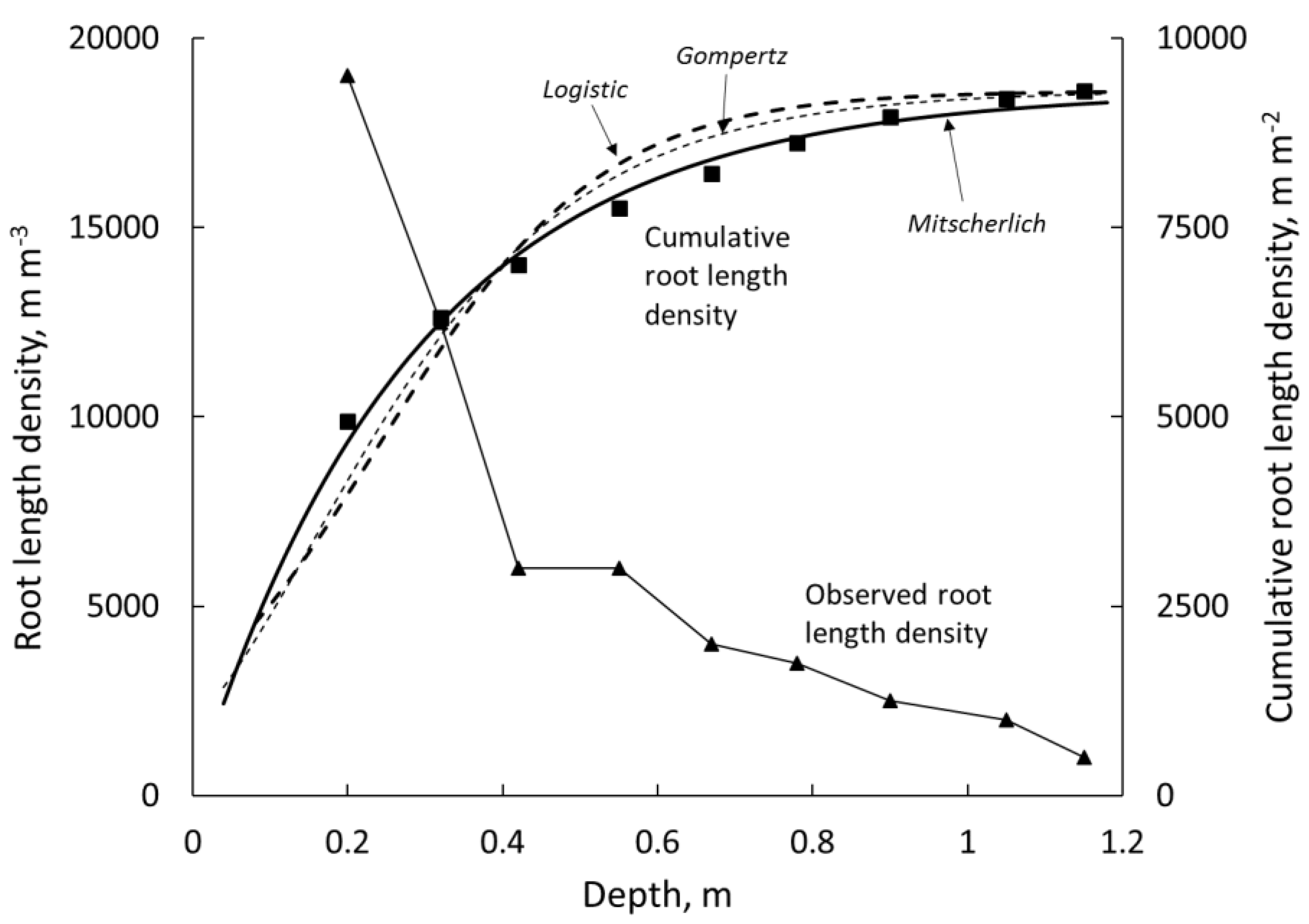
2.4. Parameter Estimation and Model Selection

Using the methodology and based on the assumption that different measurement procedures yield results which are linearly proportional to each other and therefore do not modify the shape of the R profile, the root density data were (numerically, with steps of 1 cm) integrated over depth to yield the cumulative root length density distribution (Equation (1)).

We analyzed the data using the four sigmoid functions from Table 1: the generalized logistic (Equation (2)), its two special cases (Equations (4) and (12)), and the Gompertz equation (Equation (14)), using the GENSTAT directive “fitcurve” [49]. The cumulative root density distribution was fitted including the implicit data pair (D = 0; R = 0). Figure 2 illustrates the data required for an average root density profile using data for wheat from literature [50] and illustrating the fit of the Logistic, Mitscherlich, and Gompertz function.

The use of the cumulative density distribution removes the possibility to estimate parameter confidence intervals, as errors are no longer independent. Parameter confidence intervals can be calculated using the parameters estimated from the cumulative distribution values as initial estimates in fitting the root length density functions. For comparison purposes, the fitted parameters for each of the functions were converted to D₅₀ and D₉₅ values using the equations given in Table 1. With D₅₀ and D₉₅ values we could then employ Equation (11) to calculate the parameter c for the logistic dose response function (Equation (7)).

We evaluated the fit of the four functions in terms of the fraction of variance explained, the number of cases in which convergence of the parameter estimates was achieved, and the number of times the estimated D₉₅ for a given function was below the maximum measurement depth. This number was interpreted as the risk of extrapolation.

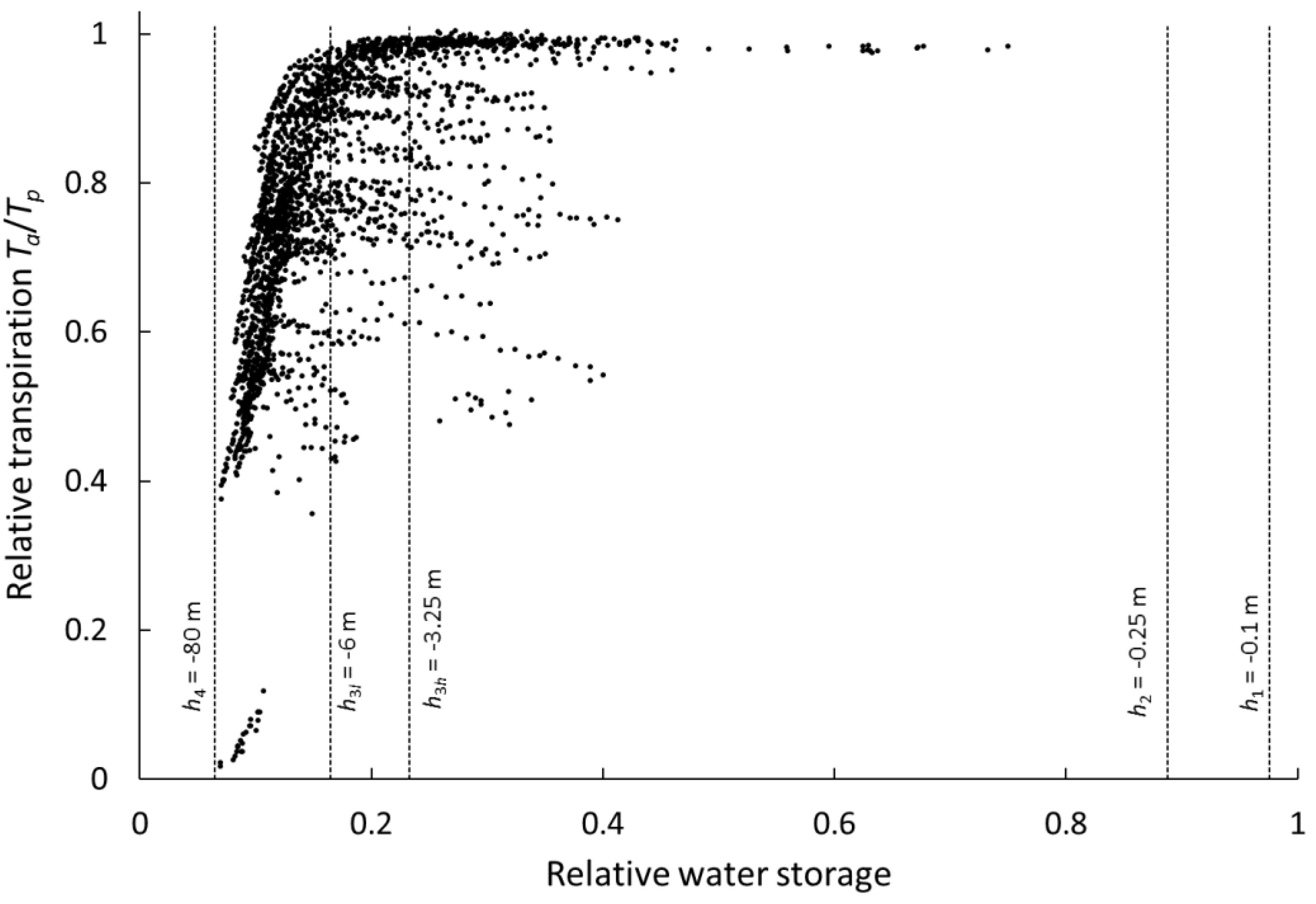
2.5. Sensitivity of Agro-Hydrological Model Output to Root Profile Shape

To evaluate the effect of the shape of root length density profiles on transpiration, simulations were performed with the SWAP model [10], version 4.01, for a maize crop grown under subtropical climate conditions. SWAP is a 1-D agro-hydrological model that numerically solves the Richards equation with a root water extraction sink term describing water flow in the soil-plant-atmosphere environment:

$$\frac{\partial \theta }{\partial t}=\frac{\partial }{\partial z}\left[K\left(h\right)\left(\frac{\partial h}{\partial z}+1\right)\right]-S\left(h\right)$$

(21)

where t denotes time (d), z is the vertical coordinate taken positive upwards (m), θ is the volumetric water content (m³·m⁻³), h is the pressure head (m), K(h) is the hydraulic conductivity (m d⁻¹), and S(h) represents water uptake by plant roots (d⁻¹). Numerically solving Equation (21) requires the knowledge of unsaturated soil hydraulic properties (K-θ-h), which were described using the analytical functions defined by the van Genuchten-Mualem model [51,52]:

$$\mathsf{\Theta }={\left[1+{\left|\alpha h\right|}^n\right]}^{(1/n)-1}$$

(22)

$$K=K_s{\mathsf{\Theta }}^{\lambda }{\left[1-{\left(1-\mathsf{\Theta }{}^{n/(n-1)}\right)}^{1-(1/n)}\right]}^2$$

(23)

where Θ = (θ − θ_r)/(θ_s − θ_r) is the effective saturation, θ_r is the residual water content (m³·m⁻³), θ_s is the saturated water content (m³·m⁻³), K is the unsaturated hydraulic conductivity (m d⁻¹), K_s is the saturated hydraulic conductivity (m·d⁻¹), and α (m⁻¹), n (-), and λ (-) are shape parameters.

The root water uptake term S(h) in Equation (21) was estimated by the piecewise linear function proposed by [53], where T_act (m·d⁻¹) is calculated by multiplying the potential transpiration T_p (m·d⁻¹) by a semi-empirical factor ε_z, evaluated for each of Z soil layers and weighted by the layer thickness w_z (m) and the root length density (ρ_z, m⁻²):

$$T_{act}=T_P{\displaystyle \sum _{z=1}^z\left[{\epsilon }_z{w}_z\frac{{\rho }_z}{{\displaystyle \sum _{z=1}^z{w}_z{\rho }_z}}\right]}$$

(24)

The multiplicative reduction factor ε_z in Equation (24) is defined by four pressure heads (0 ≥ h₁ > h₂ > h₃ > h₄) delimiting five phases of uptake. In the permanent wilting phase, (h < h₄), ε_z = 0. In the falling rate phase (h₄ < h < h₃), ε_z = (h − h₄)/(h₃ − h₄). In the constant (optimum) rate phase delimited by h₃ and h₂, ε_z = 1. In the wet phase (h₂ < h < h₁), ε_z = (h − h₁)/(h₂ − h₁). In the anaerobic phase, (h > h₁), ε_z = 0. Standard limiting pressure head values for maize [54] were used (h₁ = −0.1 m; h₂ = 0.25 m; h_3h = −3.25 m; h_3l = −6.0 m; h₄ = −80 m, h_3h corresponding to a potential transpiration rate of 5 mm·d⁻¹ or higher, h_3l corresponding to a potential transpiration rate of 1 mm·d⁻¹ or lower).

We performed the simulations for a 38-year period (1978–2015), using daily weather data from the University of São Paulo weather station, located in Piracicaba, Brazil (22.703° S; 47.624° W), representing the subtropical winter-dry climate of southeast Brazil (Köppen Cwa). For the considered period, average yearly rainfall was 1316 mm ± 242 mm (± standard deviation). The driest year (1978) showed 874 mm of rainfall, the wettest year was 1983 with 2018 mm. In this climate, rainfall is concentrated between October and March, whereas the dry months April–September correspond to less than 25% of annual rainfall.

Given the availability of crop parameters, simulations were performed for maize, which is one of the most important crops worldwide as well as for Brazilian agriculture [48]. We considered two growing seasons, maize sown on October 1 and harvested on February 28 (“summer maize” growing during the rainy season), as well as maize sown on February 15 and harvested on June 15 (“autumn maize”, dry season). For these two growing seasons, average potential evapotranspiration was 4.0 ± 1.3 mm·d⁻¹ and 2.7 ± 1.0 mm·d⁻¹, respectively. Typical soils in the region show deep groundwater levels (>5 m) and deep drainage was considered as lower boundary condition. Soil hydraulic properties from a Typic hapludox in Piracicaba, São Paulo state, Brazil (22° 42′ S, 47° 38′ W) were used. Clay content is 0.19 kg·kg⁻¹ in the 0–0.30 m layer and 0.26 kg·kg⁻¹ below that. Bulk density increases from 1400 kg·m⁻³ in the top layer to around 1650 kg·m⁻³ in the subsoil. The parameters describing the soil hydraulic properties, θ(h) and K(h), according to the Van Genuchten-Mualem analytical functions [51,52] used in our simulations are shown in

Table 3. Hydraulic parameters for Van Genuchten-Mualem analytical functions [51,52] used in the SWAP simulations.

Depth (m)	θr	θs	α (m−1)	n	λ	Ks (m·d−1)
0.00–0.30	0.01	0.43	2.27	1.548	−1.983	0.1965
0.30–2.00	0.02	0.38	2.14	2.075	−1.039	0.2556

.

A fixed period of 60 days was simulated from emergence (development stage DVS = 0) to anthesis (DVS = 1), and an additional 60 days from anthesis (DVS = 1) to maturity (DVS = 2). The root length density profile was described according to the logistic dose response function (Equation (7)), for different parameter scenarios, consisting of three values for c (−1, −3, and −5) combined to three values for D₅₀ (0.15 m, 0.30 m, and 0.45 m), resulting in 3 × 3 = 9 scenarios. The logistic dose response function was selected for this simulation step mainly due to its preference in root distribution studies (e.g., [35]).

Leaf area index, rooting depth, and crop height were defined as piecewise linear functions of development stage according to data points in

Table 4. Leaf area index, crop height, and rooting depth as a function of development stage used in SWAP simulations with maize. Values retrieved from [55] and from standard SWAP input file.

Development Stage	Leaf Area Index (m2 m−2)	Crop Height (m)	Rooting Depth (m)
0	0.05	0.01	0.05
0.30	0.14	0.15	0.2
0.50	0.61	0.40	0.5
0.70	4.1	1.40	0.8
1.0	5.0	1.70	0.9
1.4	5.8	1.80	0.9
2.0	5.2	1.75	0.9

.

Other parameters referring to the maize crop used in our simulation are shown in

Table 5. Crop growth parameters used in the simple crop module used in the SWAP model.

Description	Parameter	Value	Unit
Plant maximum height	Hmax	175	cm
Reflection coefficient, Albedo	Cref	0.20	‒
Minimum canopy resistance	RSC	131	s m−1
Extinction coefficient for diffuse visible light	Kdif	0.60	‒
Extinction coefficient for direct visible light	Kdir	0.75	‒
Length of crop cycle - fixed	LCC	120	d
Interception coefficient Von Hoyningen-Hune and Braden	COFAB	0.25	cm

. These parameter values are part of the standard parameterization for the simple crop module of maize embedded in the SWAP model and more details on this parameterization can be found in [55,56].

Model output was analyzed regarding the relative transpiration T_a/T_p, an indicator of overall crop water stress, for the nine scenarios of root length density profile shapes. It is worth noting that relative transpiration is often considered proportional to relative yield [57,58].

3. Results

3.1. Function Selection and Parameter Values

Table 6. Descriptive results for the four sigmoid functions used as a criterion to define a preference for a fitting function.

Sigmoid Function	Convergence (n = 570)	D95 > Dmax	R2adj	Mean D50 (m)	Mean D95 (m)
Generalized logistic (Equation (2))	54	5	1.00	0.322	0.644
Logistic (Equation (4))	568	48	0.98	0.267	0.560
Exponential (Equation (12))	568	422	0.98	0.460	1.942
Gompertz (Equation (14))	568	174	0.99	0.272	0.699

contains the descriptive results used as a criterion to define a preference for a fitting function.

Using the convergence of the estimate, the goodness of fit, the conservative properties in terms of extrapolation (D₉₅ greater than maximum measurement depth), and consistency of analysis in terms of existing databases, notably that presented by [35], the logistic function (Equation (4)) was selected for further analyses.

A summary of the results for the different growth curves is given in

Table 7. Mean D₅₀ and D₉₅ calculated by the logistic function (Equation (4)) using n observations and minimum half-distance r_n calculated using n_r observations. Parameter c from the logistic dose response function (Equation (7)) was calculated by Equation (11).

Crop	D50 (± Standard Error) (m)	D95 (± Standard Error) (m)	n	rn (± Standard Error) (mm)	nr	c	Rx (mm−1)
All crops	0.27 (±0.24)	0.56 (±0.48)	568	5.6 (±5.7)	494	−3.969	10.2
Wheat	0.22 (±0.10)	0.49 (±0.25)	80	6.4 (±6.1)	50	−3.677	8.5
Maize	0.39 (±0.20)	0.80 (±0.40)	48	6.5 (±4.7)	40	−4.071	7.4
Rice	0.13 (±0.07)	0.27 (±0.13)	87	5.2 (±5.3)	87	−4.048	11.6
Barley	0.17 (±0.06)	0.33 (±0.09)	10	4.8 (±3.7)	7	−4.286	12.9
Soybean	0.27 (±0.17)	0.60 (±0.33)	42	7.1 (±8.0)	40	−3.716	6.8
Pulses	0.28 (±0.12)	0.59 (±0.25)	39	4.7 (±0.7)	37	−3.942	14.6
Cotton	0.32 (±0.10)	0.67 (±0.22)	97	5.4 (±1.3)	97	−3.989	10.9
Potato	0.32 (±0.06)	0.62 (±0.13)	40	3.2 (±0.6)	40	−4.482	27.7
Sunflower	0.35 (±0.19)	0.79 (±0.46)	26	4.3 (±1.2)	23	−3.596	19.1
Rye	0.22 (±0.06)	0.47 (±0.13)	7	4.6 (±2.1)	6	−3.955	15.2
Rapeseed	0.18 (±0.04)	0.39 (±0.09)	30	2.7 (±0.9)	21	−3.858	45.3
Sugar beet	0.48 (±0.15)	0.95 (±0.28)	13	3.9 (±1.8)	7	−4.349	19.2
Other	0.28 (±0.18)	0.56 (±0.37)	49	10.3 (±13.3)	39	−4.194	2.9

. In this table, parameter values are pooled over different measurement types (counts, weights and lengths) based on the comparison between the different measurement procedures, as discussed in [35]. Parameters for the mean root half-distance approximation were calculated by Equation (19), based on measurements of root length densities alone.

Calculating the parameter confidence intervals using parameters estimates as initial values for root length density function fits led to data loss due to non-convergence. A note of caution should be added here: Given the non-linear relationship, use of average D₅₀ and D₉₅ values will yield results that are different from those obtained through using the individual parameter values and then averaging the profile.

3.2. Sensitivity of Agro-Hydrological Model Output to Root Profile Shape

Figure 3 was produced from the daily output of simulation results obtained with the SWAP model for autumn maize, grown yearly between 1978–2015, under weather conditions of Piracicaba-SP, Brazil, using root density profiles described by the logistic dose-response function (Equation (7)) for the scenario with D₅₀ = 0.30 m and c = −1. In this figure, the relative water storage was calculated as the soil water storage between the surface and 0.9 m depth, divided by the corresponding saturated water content. Figure 3 also shows the relative water storage corresponding to the Feddes reduction function [53] threshold values h₁, h₂, h_3h, h_3l, and h₄.

In

Table 8. Average difference between T_a/T_p simulated using root density profiles described by the logistic dose response function (Equation (7)) with different parameter combinations (D₅₀ and c) compared with the scenario of D₅₀ = 0.45 m and c = −1, based on 38 maize crop cycles (autumn maize and summer maize) between 1978 and 2015 in Piracicaba, Brazil. Values between brackets are the respective coefficients of variation over the 38 years.

	Autumn Maize (February–June)			Summer Maize (November–February)
D50 (m)	0.15	0.30	0.45	0.15	0.30	0.45
c = −1	0.017 (23%)	0.006 (23%)	0	0.010 (53%)	0.004 (65%)	0
c = −3	0.049 (17%)	0.035 (18%)	0.019 (22%)	0.030 (48%)	0.018 (56%)	0.008 (68%)
c = −5	0.053 (16%)	0.041 (18%)	0.026 (21%)	0.033 (47%)	0.021 (56%)	0.011 (68%)

, the average difference between T_a/T_p of respective parameter combinations and the value obtained for the D₅₀ = 0.45 m and c = −1 scenario are shown together with the coefficients of variation (in the order of 20% for autumn maize and 50–60% for summer maize).

4. Discussion

Due to the lack of data at small depths, in combination with the additional shape parameter, the generalized logistic function showed convergence for less than 10% of all database. The other three equations fitted well to observed data, with high regression coefficient, and convergence for almost all observed database (Table 6). Of these, the logistic function offered the best descriptive quality, with a relatively low risk of an extrapolation error; that is, in most cases the parameter D₉₅ was smaller than the maximum measurement depth. An alternative is the Gompertz equation, although with a higher frequency of D₉₅ > D_max than the logistic function. In its turn, the exponential Mitscherlich equation resulted in an extrapolation error (D₉₅ > D_max) in 75% of the cases.

Defining the effective root zone as the depth above which most of the roots are concentrated [59], we can use the value of D₉₅ of Table 6 estimated by the logistic function as a proxy of this parameter. In general, the values of D₉₅ were similar among crops, with maize and sugar beet showing the deepest roots. With analogous analysis for crops from temperate regions, [59] found deeper root systems for similar crops. Although the estimated D₉₅ values from both studies are within the range usually reported in the literature, our analysis covered 568 soil profiles against 96 of the analysis performed by [59]. According to Table 7, the highest value recorded for parameter c was for sunflower (−3.6) and the lowest value for potato (−4.5). A more negative c value leads to a more concentrated distribution of roots around D₅₀.

Regarding the agro-hydrological simulations, several engineering models relate transpiration reduction to water content, soil water storage or related quantities using simple linear relations with some threshold values, the probably most well-known is the one published in a FAO handbook [7]. However, such a relationship is only partially supported by the simulation results shown in Figure 3. Our simulation results obtained with the SWAP model [10] for maize grown yearly between 1978–2015, showed overall T_a/T_p values for summer maize between 0.84 and 0.88, obviously higher than for autumn maize (from 0.59 to 0.64). For both cropping seasons, the highest values were obtained with the D₅₀ = 0.45 m and c = −1 scenario, representing the most even distribution of roots over depth (Figure 1). The lowest values were obtained for the D₅₀ = 0.15 m and c = −5 scenario, representing the most concentrated roots distribution around D₅₀.

Although the differences in average values of T_a/T_p among the scenarios were relatively small (up to 5% for autumn maize and 3% for summer maize), they were consistent over the years, especially for autumn maize growing under predominantly drier conditions. The scatter in Figure 3 data points is explained by two facts: (1) the SWAP model employs two values for the threshold pressure head h₃, in which h_3h corresponds to conditions with a high (≥5 mm d⁻¹) T_p, and h_3l to a low (≤1 mm d⁻¹) T_p; for intermediate values of T_p, h₃ is linearly interpolated. This will cause some horizontal scattering of data points between both h₃ values; (2) pressure heads are unlikely to be the same at all depths, and roots are unevenly distributed over depth. Consequently, identical relative water storage values may be reached from different water content and pressure head distributions, thus, it may result in different transpiration reduction. This will cause a vertical scatter of data points in Figure 3, and it is likely to increase for more uneven root distributions.

The relative insensitivity of the modeling results to root length density distribution are in part due to the assumptions of the Feddes transpiration reduction function [53] as applied in the SWAP model. This reduction function does not account for root water uptake compensation, i.e., enhanced uptake from a wetter soil layer when other layers become too dry [60]. Furthermore, it only considers relative root length, not accounting for absolute root length density. It is well known that the mechanistic approaches that simulate root water uptake at a macroscopic scale (entire root system) should include the preferential zone (layers with smaller resistances) of root water uptake, e.g., wetter soil layers. In this sense, absolute root length density distribution and soil hydraulic properties are key factors for more consistent simulations. The importance of these issues for root water uptake modeling has been discussed in [23,24,61,62].

5. Conclusions

We tested the quality of fit of some descriptive functions used to simulate root length density distribution over depth by fitting to experimentally established crop root density profiles retrieved from literature. We also assessed the importance of the shape of the root length density profile in hydrological modeling by testing the sensitivity of actual transpiration predictions to shape parameters of root length density functions.

More than 50 literature sources were retrieved with 568 sets of root density profiles for crop species that together represent 77% of the cropped area in the world. We found the cumulative root density distributions to be well described by the logistic function (average $R_{adj}^2$ of 0.98) or the Gompertz function (average $R_{adj}^2$ of 0.99). The simulation case study showed that root length density distribution has a consistent effect on relative transpiration, which is frequently assumed proportional to relative yield. The analysis of detailed day-to-day relative transpiration showed that the approach commonly used in irrigation science to predict transpiration reduction and irrigation requirement from soil water storage or average water content is only partially supported by our simulation results.

References

1. Hartmann, A.; Šimůnek, J.; Aidoo, M.K.; Seidel, S.J.; Lazarovitch, N. Implementation and application of a root growth module in Hydrus. Vadose Zone J. 2018, 17, 170040. [Google Scholar] [CrossRef]
2. Schnepf, A.; Leitner, D.; Landl, M.; Lobet, G.; Mai, T.H.; Morandage, S.; Sheng, C.; Zörner, M.; Vanderborght, J.; Vereecken, H. CRootBox: A structural-functional modelling framework for root systems. Ann. Bot. 2018, 121, 1033–1053. [Google Scholar] [CrossRef] [PubMed]
3. Sellers, P.J.; Dickinson, R.E.; Randall, D.A.; Betts, A.K.; Hall, F.G.; Berry, J.A.; Collatz, G.J.; Denning, A.S.; Mooney, H.A.; Nobre, C.A.; et al. Modeling the exchanges of energy, water, and carbon between continents and the atmosphere. Science 1997, 275, 502–509. [Google Scholar] [CrossRef] [PubMed]
4. Pitman, A.J. The evolution of, and revolution in, land surface schemes designed for climate models. Int. J. Climatol. 2003, 23, 479–510. [Google Scholar] [CrossRef]
5. Ferguson, I.M.; Jefferson, J.L.; Maxwell, R.M.; Kollet, S.J. Effects of root water uptake formulation on simulated water and energy budgets at local and basin scales. Environ. Earth Sci. 2016, 75, 316. [Google Scholar] [CrossRef]
6. Zeng, X.; Dai, Y.J.; Dickinson, R.E.; Shaikh, M. The role of root distribution for climate simulation over land. Geophys. Res. Let. 1998, 25, 4533–4536. [Google Scholar] [CrossRef]
7. Doorenbos, J.; Pruitt, W.O. Guidelines for Predicting Crop Water Requirements; Irrigation and Drainage Paper 24; Food and Agriculture Organization of the United Nations: Rome, Italy, 1975; p. 179. [Google Scholar]
8. Bouman, B.A.M.; Van Keulen, H.; Van Laar, H.H.; Rabbinge, R. The ‘School of de Wit’ crop growth simulation models: A pedigree and historical overview. Agric. Syst. 1996, 52, 171–198. [Google Scholar] [CrossRef]
9. Šimůnek, J.; van Genuchten, M.T.; Šejna, M. Recent developments and applications of the HYDRUS computer software packages. Vadose Zone J. 2016, 15. [Google Scholar] [CrossRef]
10. Kroes, J.G.; Van Dam, J.C.; Bartholomeus, R.P.; Groenendijk, P.; Heinen, M.; Hendriks, R.F.A.; Mulder, H.M.; Supit, I.; Van Walsum, P.E.V. SWAP Version 4: Theory and Description of User Manual; Report 2780; Wageningen Environmental Research: Wageningen, The Netherlands, 2017. [Google Scholar]
11. Bonfante, A.; Terribile, F.; Bouma, J. Refining physical aspects of soil quality and soil health when exploring the effects of soil degradation and climate change on biomass production: An Italian case study. Soil 2019, 5, 1–14. [Google Scholar] [CrossRef]
12. Bar-Tal, A.; Ganmore-Neumann, R.; Ben-Hayyim, G. Root architecture effects on nutrient uptake. In Basic Life Sciences: Biology of Root Formation and Development; Altman, A., Waisel, Y., Eds.; Springer: Boston, MA, USA, 1997; Volume 65. [Google Scholar]
13. Doussan, C.; Pages, L.; Pierret, A. Soil exploration and resource acquisition by plant roots: An architectural and modelling point of view. In Sustainable Agriculture, 1st ed.; Lichtfouse, E., Navarrete, M., Debaeke, P., Véronique, S., Alberola, C., Eds.; Springer: Dordrecht, The Netherlands, 2003; pp. 419–431. [Google Scholar]
14. Wu, L.; McGechan, M.B.; Watson, C.A.; Baddeley, J.A. Developing existing plant root system architecture models to meet future agricultural challenges. Adv. Agron. 2005, 41, 91–145. [Google Scholar]
15. Wang, H.; Inukai, Y.; Yamauchi, A. Root development and nutrient uptake. Crit. Rev. Plant Sci. 2006, 25, 279–301. [Google Scholar] [CrossRef]
16. Darrah, P.R.; Jones, D.L.; Kirk, G.J.D.; Roose, T. Modelling the rhizosphere: A review of methods for ‘upscaling’ to the whole-plant scale. Eur. J. Soil Sci. 2006, 57, 13–25. [Google Scholar] [CrossRef]
17. Schneider, C.L.; Attinger, S.; Delfs, J.O.; Hildebrandt, A. Implementing small scale processes at the soil-plant interface—The role of root architectures for calculating root water uptake profiles. Hydrol. Earth Syst. Sci. 2010, 14, 279–289. [Google Scholar] [CrossRef]
18. Paez-Garcia, A.; Motes, C.M.; Scheible, W.R.; Chen, R.; Blancaflor, E.B.; Monteros, M.J. Root traits and phenotyping strategies for plant improvement. Plants 2015, 4, 334–355. [Google Scholar] [CrossRef] [PubMed]
19. Rasmussen, I.S.; Dresbøll, D.B.; Thorup-Kristensen, K. Winter wheat cultivars and nitrogen (N) fertilization—Effects on root growth, N uptake efficiency and N use efficiency. Eur. J. Agron. 2015, 68, 38–49. [Google Scholar] [CrossRef]
20. Shahzad, Z.; Amtmann, A. Food for thought: How nutrients regulate root system architecture. Curr. Opin. Plant Biol. 2017, 39, 80–87. [Google Scholar] [CrossRef] [PubMed]
21. Feddes, R.A.; Raats, P.A.C. Parameterizing the soil-water-plant root system. In Unsaturated-Zone Modeling: Progress, Challenges and Applications; Feddes, R.A., de Rooij, G.H., van Dam, J.C., Eds.; Wageningen UR Frontis Series: Dordrecht, The Netherlands, 2004; pp. 95–141. [Google Scholar]
22. De Willigen, P.; Heinen, M.; Kirkham, M.B. Transpiration and root water uptake. In Encyclopedia of Hydrological Sciences; Anderson, M.H., Ed.; John Wiley and Sons: London, UK, 2005; Chapter 70. [Google Scholar]
23. De Jong van Lier, Q.; Metselaar, K.; Van Dam, J.C. Root water extraction and limiting soil hydraulic conditions estimated by numerical simulation. Vadose Zone J. 2006, 5, 1264–1277. [Google Scholar] [CrossRef]
24. De Jong van Lier, Q.; Van Dam, J.C.; Durigon, A.; Dos Santos, M.A.; Metselaar, K. Modeling water potentials and flows in the soil–plant system comparing hydraulic resistances and transpiration reduction functions. Vadose Zone J. 2013, 12, 1–20. [Google Scholar] [CrossRef]
25. Raats, P.A.C. Uptake of water from soils by plant roots. Transp. Porous Med. 2007, 68, 5–28. [Google Scholar] [CrossRef] [Green Version]
26. Diggle, A.J. ROOTMAP—A model in three-dimensional coordinates of the growth and structure of fibrous root systems. Plant Soil 1998, 105, 169–178. [Google Scholar] [CrossRef]
27. Couvreur, V.; Vanderborght, J.; Javaux, M. A simple three-dimensional macroscopic root water uptake model based on the hydraulic architecture approach. Hydrol. Earth Syst. Sci. 2012, 16, 2957–2971. [Google Scholar] [CrossRef] [Green Version]
28. Van Noordwijk, M.; Van de Geijn, S.C. Root, shoot and soil parameters required for process-oriented models of crop growth limited by water or nutrients. Plant Soil 1996, 183, 1–25. [Google Scholar] [CrossRef]
29. De Jong van Lier, Q.; Van Dam, J.C.; Metselaar, K.; de Jong, R.; Duijnisveld, W.H.M. Macroscopic root water uptake distribution using a matric flux potential approach. Vadose Zone J. 2008, 7, 1065–1078. [Google Scholar] [CrossRef]
30. Gerwitz, A.; Page, E.R. An empirical mathematical model to describe plant root systems. J. Appl. Ecol. 1974, 11, 773–781. [Google Scholar] [CrossRef]
31. O’Toole, J.C.; Bland, W.L. Genotypic variation in crop plant root systems. Adv. Agron. 1987, 85, 181–219. [Google Scholar]
32. Zuo, Q.; Jie, F.; Zhang, R.; Meng, L. A generalized function of wheat’s root length density distributions. Vadose Zone J. 2004, 3, 271–277. [Google Scholar] [CrossRef]
33. Hodgkinson, L.; Dodd, I.C.; Binley, A.; Ashton, R.W.; White, R.P.; Watts, C.M.; Whalley, W.R. Root growth in field-grown winter wheat: Some effects of soil conditions, season and genotype. Eur. J. Agron. 2017, 91, 74–83. [Google Scholar] [CrossRef]
34. Jackson, R.B.; Canadell, J.; Ehleringer, J.R.; Mooney, H.A.; Sala, O.E.; Schulze, E.D. A global analysis of root distributions for terrestrial biomes. Oecologia 1996, 108, 389–411. [Google Scholar] [CrossRef]
35. Schenk, H.J.; Jackson, R.B. The global biogeography of roots. Ecol. Monogr. 2002, 72, 311–328. [Google Scholar] [CrossRef]
36. Van Wijk, M.T. Understanding plant rooting patterns in semi-arid systems: An integrated model analysis of climate, soil type and plant biomass. Glob. Ecol. Biogeogr. 2011, 20, 331–342. [Google Scholar] [CrossRef]
37. Benjamin, J.G.; Nielsen, D.C. Water deficit effects on root distribution of soybean, field pea and chickpea. Field Crops Res. 2006, 97, 248–253. [Google Scholar] [CrossRef]
38. Ober, E.S.; Sharp, R.E. Regulation of root growth responses to water deficit. In Advances in Molecular Breeding toward Drought and Salt Tolerant Crops; Jenks, M.A., Ed.; Springer: Dordrecht, The Netherlands, 2007; pp. 33–53. [Google Scholar]
39. Saidi, A.; Ookawa, T.; Hirasawa, T. Responses of root growth to moderate soil water deficit in wheat seedlings. Plant Prod. Sci. 2010, 13, 261–268. [Google Scholar] [CrossRef]
40. Schenk, H.J.; Jackson, R.B. Mapping the global distribution of deep roots in relation to climate and soil characteristics. Geoderma 2005, 126, 129–140. [Google Scholar] [CrossRef]
41. Stalham, M.A.; Allen, E.J. Effect of variety, irrigation regime and planting date on depth, rate, duration and density of root growth in the potato (Solanum tuberosum) Crop. J. Agric. Sci. 2001, 137, 251–270. [Google Scholar] [CrossRef]
42. France, J.; Thornley, J.H.M. Mathematical Models in Agriculture: A Quantitative Approach to Problems in Agriculture and Related Sciences; University of Chicago Press: Chicago, IL, USA, 1985; p. 335. [Google Scholar]
43. Richards, J.R. A flexible growth function for empirical use. J. Exp. Bot. 1959, 10, 290–300. [Google Scholar] [CrossRef]
44. Verduin, J. Baule-Mitscherlich limiting factor equation. Science 1953, 117, 392. [Google Scholar] [CrossRef] [PubMed]
45. De Willigen, P.; Heinen, M.; Mollier, A.; Van Noordwijk, M. Two-dimensional growth of a root system modelled as a diffusion process. I. Analytical solutions. Plant Soil 2002, 240, 225–234. [Google Scholar] [CrossRef]
46. Gardner, W.R. Dynamic aspects of water availability to plants. Soil Sci. 1960, 89, 63–73. [Google Scholar] [CrossRef]
47. Jin, K.; Shen, J.; Ashton, R.W.; Dodd, I.C.; Parry, M.A.J.; Whalley, W.R. How do roots elongate in a structured soil? J. Exp. Bot. 2013, 64, 4761–4777. [Google Scholar] [CrossRef]
48. Leff, B.; Ramankutty, N.; Foley, J.A. Geographic distribution of major crops across the world. Glob. Biogeochem. 2004, 18. [Google Scholar] [CrossRef]
49. GenStat Committee. GenStat® Release 7.1 Reference Manual Part 2: Directives; VSN Int.: Oxford, UK, 2003. [Google Scholar]
50. Mian, M.A.R.; Nafziger, E.D.; Kolb, F.L.; Teyker, R.H. Root size and distribution of field-grown wheat genotypes. Crop Sci. 1994, 34, 810–812. [Google Scholar] [CrossRef]
51. Van Genuchten, M.T. A closed-form equation for predicting the hydraulic conductivity of unsaturated soils. Soil Sci. Soc. Am. J. 1980, 44, 892–897. [Google Scholar] [CrossRef]
52. Mualem, Y. A new model for predicting the hydraulic conductivity of unsaturated porous media. Water Resour. Res. 1976, 12, 513–522. [Google Scholar] [CrossRef] [Green Version]
53. Feddes, R.A.; Kowalik, P.J.; Zaradny, H. Simulation of Field Water Use and Crop Yield; Simulation Monograph Series; PUDOC: Wageningen, The Netherlands, 1978. [Google Scholar]
54. Taylor, S.A.; Ashcroft, G.M. Physical Edaphology; Freeman and Co.: San Francisco, CA, USA, 1972; pp. 434–435. [Google Scholar]
55. Boons-Prins, E.R.; De Koning, G.H.J.; Van Diepen, C.A.; Penning de Vries, F.W.T. Crop-Specific Parameters for Yield Forecasting across the European Community; Simulation Reports CABO-TT, No. 32; Wageningen University & Research: Wageningen, The Netherlands, 1993; p. 160. [Google Scholar]
56. Pinto, V.M.; van Dam, J.C.; de Jong van Lier, Q.; Reichardt, K. Intercropping simulation using the SWAP model: Development of a 2x1D Algorithm. Agriculture 2019, 9, 126. [Google Scholar] [CrossRef]
57. Steduto, P.; Hsiao, T.C.; Fereres, E.; Raes, D. Crop Yield Response to Water; FAO Irrigation and Drainage Paper 66; Food and Agriculture Organization of the United Nations: Rome, Italy, 2012; p. 500. [Google Scholar]
58. Greaves, G.E.; Wang, Y. Yield response, water productivity, and seasonal water production functions for maize under deficit irrigation water management in southern Taiwan. Plant Prod. Sci. 2017, 20, 353–365. [Google Scholar] [CrossRef] [Green Version]
59. Fan, J.; McConkey, B.; Wang, H.; Janzen, H. Root distribution by depth for temperate agricultural crops. Field Crops Res. 2016, 189, 68–74. [Google Scholar] [CrossRef] [Green Version]
60. Jarvis, N.J. Simple physics-based models of compensatory plant water uptake: Concepts and eco-hydrological consequences. Hydrol. Earth Syst. Sci. 2011, 15, 3431–3446. [Google Scholar] [CrossRef]
61. Dos Santos, M.A.; De Jong van Lier, Q.; Van Dam, J.C.; Bezerra, A.H.F. Benchmarking test of empirical root water uptake models. Hydrol. Earth Syst. Sci. 2017, 21, 473–493. [Google Scholar] [CrossRef] [Green Version]
62. Moraes, M.T.; Bengough, A.G.; Debiasi, H.; Franchini, J.C.; Levien, R.; Schnepf, A.; Leitner, D. Mechanistic framework to link root growth models with weather and soil physical properties, including example applications to soybean growth in Brazil. Plant Soil 2018, 428, 67–92. [Google Scholar] [CrossRef] [Green Version]
Figure 1. Logistic dose response function (A) and its derivative (B) for parameter value D50 = 0.3 and c = −1, −3, and −5.
Soilsystems 03 00044 g001
Figure 2. Measured root length density data [50] numerically integrated to yield the cumulative root density distribution R (m m−3) and fitted using different monotonic sigmoid functions.
Soilsystems 03 00044 g002
Figure 3. Relative transpiration (Ta/Tp) as a function of effective saturation Se obtained from SWAP simulations using root density profiles described by the logistic dose-response function (Equation (7)) with D50 = 0.30 m and c = −1 scenario, based on 38 autumn maize crop cycles between 1978 and 2015.
Soilsystems 03 00044 g003