Gauge Dependence of the Gauge Boson Projector


Institute of Physics, University of Tartu, W. Oswaldi 1, 50411 Tartu, Estonia
*
Author to whom correspondence should be addressed.
Particles 2020, 3(3), 543-561; https://doi.org/10.3390/particles3030037
Submission received: 5 June 2020
/
Accepted: 24 July 2020
/
Published: 28 July 2020
Abstract
:The propagator of a gauge boson, like the massless photon or the massive vector bosons and Z of the electroweak theory, can be derived in two different ways, namely via Green’s functions (semi-classical approach) or via the vacuum expectation value of the time-ordered product of the field operators (field theoretical approach). Comparing the semi-classical with the field theoretical approach, the central tensorial object can be defined as the gauge boson projector, directly related to the completeness relation for the complete set of polarisation four-vectors. In this paper we explain the relation for this projector to different cases of the gauge and explain why the unitary gauge is the default gauge for massive gauge bosons.
1. Introduction
As it is familiar for the scalar and Dirac propagators, the propagator of the vector boson V between two space-time locations x and y can be considered as a two-point correlator, that is, as the vacuum expectation value of the time ordered product of the vector potential at these two locations,
However, in order to get to the momentum space representation of this propagator, one needs to use the completeness relation for the polarisation four-vectors. This is not an easy task, as this completeness relation is not given uniquely for a complete set of four polarisation states. As it is well known, a massless vector boson like the photon has two polarisation states. For a massive vector boson ( or Z), in addition there is a longitudinal polarisation state. However, the addition of a time-like polarisation state is not unique and depends on the gauge we use, as we will show in this paper. In order to get to this point, we construct the propagator of the vector boson in a semi-classical way as Green’s function obeying the canonical equation of motion, derived as Euler–Lagrange equation from the Lagrange density containing a gauge fixing term,
a result which will be derived in Section 5. is the gauge parameter in general gauge. The solution of the Euler–Lagrange equation leads to a propagator
with a definite second rank tensor structure which we call the gauge boson projector. is the Minkowski metric.
The paper is organised as follows. In Section 2 we introduce the gauge boson projector. As a naive extension of the completeness relation for the polarisation vectors fails, we offer a pragmatic solution which will be explained in the following. In Section 3 we start with the Lagrange density of the photon and explain why the solution of the corresponding Euler–Lagrange equation needs a gauge fixing term. For a general gauge we solve the equation for the Green’s function. A recourse to historical approaches is needed to understand the occurence of primary and secondary constraints. In Section 4 the quantisation of the photon field is continued in a covariant manner. In Section 5 we explain the appearance of a mass term via the Higgs mechanism and the restriction of the gauge degrees of freedom in this case, leading to the unitary gauge as the default setting for massive vector bosons. In Section 6 we explain and give an example for the gauge independence of physical processes. Our conclusions and outlook are found in Section 7. For the basics we refer to References [1,2,3,4,5].
2. The Gauge Boson Projector
The gauge boson projector as central tensorial object in Equation (3) takes the simplest form for the Feynman gauge (). For Landau gauge one obtains a purely transverse projector , and for the unitary gauge one has which is transverse only on the mass shell . But why do we talk about a projector at all? A comparison with the construction of the fermion propagator can help to explain the conceptual approach employed in this paper.
2.1. Construction of the Fermion Propagator
As for the gauge boson propagator, there are in principle two ways to construct the fermion propagator. As a Green’s function the fermion propagator has to solve the equation
equivalent to the Dirac equation as the corresponding Euler–Lagrange equation. In momentum space this equation reads (with ) which can be solved by . Note that the inverse of the matrix is well defined, since . Back to configuration space one has
where we have added an infinite imaginary shift to obtain a Feynman propagator. On the other hand, the fermion propagator is defined again as two-point correlator, that is, as the vacuum expectation value of the time-ordered product of the spinor and the adjoint spinor,
where we have started with the field operators
and with the only non-vanishing antimutators
where we have used the completeness relations
and, finally, where we have used Cauchy’s theorem to write the integral in a compact four-dimensional form. The result is quite obviously the same as the one obtained via the Green’s function. Still, one might become aware of the central link, given by the completeness relations. A similar construction should work also for the gauge boson propagator.
2.2. Construction of the Gauge Boson Propagator
As for the quantisation of the fermion field operator we summed over the spin polarisation states (corresponding to up and down spin), it is natural to assume that for quantisation of the gauge boson field operator we have to sum over the polarisations . Still, the (silent) assumption that the summation runs over all possible (four) polarisation states will have to be looked over again, as it will turn out. Up to that point, we use the summation sign indexed by without specifying the set of polarisations it runs over. Therefore, starting with
with and , the calculation of the two-point correlator leads to
However, what kind of completeness relation we can use in this case? We know that there are at least two physical polarisation directions which are orthogonal to each other and at the same time orthogonal to the wave vector ,
(). , and span an orthonormal frame. Therefore, in particular the usual three-dimensional basis can be expressed in this frame,
As the usual basis is orthonormal, we conclude that
which can be rewritten as a first (three-dimensional) completeness relation,
Finally, considering as a third orthonomal polarisation vector, one obtains
where the complex conjugate has no effect on a real-valued basis but allows for the generalisation for instance to a chiral basis. (We will not make the chiral basis explicit though as we reserve for something else). A generalisation of this completeness relation to four-vectors (with time component set to zero) is straightforward and leads to
with . As before, an attempt can be done to switch the non-covariant part of the right hand side to the left hand side by defining a fourth (time-like) polarisation. However, in this simple form this attempt fails. does not give the correct sign, and the more involved trial is of no help here as the product with the conjugate will remove the effect of the imaginary unit.
2.3. The Issue of Dispersion
The canonical field quantisation in Equation (10) is based on plane waves. This issue becomes problematic if we consider a vector field complemented by a gauge fixing term, leading to a nontrivial dispersion of the solution in the case of a massive vector boson [6]. As we will see in Section 5, the Proca equation can no longer be considered as a vector extension of the Klein–Gordon equation. Instead, the mass of the vector boson depends on the gauge parameter . Accordingly, the canonical quantisation based on a particle with fixed mass cannot be applied. However, in our approach we are able to circumvent the problem related to the canonical quantisation by using Green’s functions. Note that Green’s functions are classical and, therefore, independent of the quantisation scheme.
2.4. A Pragmatic Solution
At this point we offer a pragmatic solution. As we know the explicit form of the gauge boson propagator from the Green’s function approach employed before, we conclude that
Therefore, the completeness relation depends on the gauge. The pragmatic solution tells us that for Feynman gauge for instance one obtains , independent of whether we know which polarisations are summed over and how the explicit polarisation vectors look like. However, we can speculate about how these two are related to each other. We can assure ourselves that a gauge boson on the mass shell has only vector components. In this case we obtain the Landau projector () [7,8,9]
containing only the vector component of the polarisation. Equation (19) can be explicitly seen in the rest frame of the massive vector boson. For one obtains
with , and . If the gauge boson is offshell, it is described by the unitary projector (), containing also a scalar component [8],
with as the offshellness dominating the scalar component. The appearance of the components of the metric tensor in polarisation space seems to suggest that the summation over can be understood as the contraction of covariant with contravariant components in polarisation spacetime, reserving for the polarisation vectors the role of a tetrad between ordinary spacetime and polarisation spacetime. This will be worked out in more detail in Section 4 in case of the photon (cf. Equation (42)).
3. Green’s Function of the Photon
In order to investigate the relation between completeness relation and propagator in detail, we start with the Lagrange density of the photon,
Containing only the self energy of the photon, the Euler–Lagrange equations can be obtained by variation of the action integral . One obtains
where for the last step we have used integration by parts. In order to vanish for an arbitrary variation of the gauge field, one has to claim that
However, the corresponding equation (a factor i for later convenience)
for the Green’s function cannot be solved, as the operator is not invertible. As found by Faddeev and Popov in 1967, this problem turns out to be deeply related to the gauge degree of freedom [10]. The solution for this problem is given by amending the Lagrange density by a gauge fixing term,
the introduction of which can be understood on elementary level also as the addition of a Lagrange multiplier times the square of , restricting the solutions to those which satisfy the Lorenz gauge condition proposed exactly a century earlier [11]. This condition does not fix completely the gauge but eliminates the redundant spin-0 component in the representation of the Lorentz group, leaving a gauge degree of freedom with . However, as the gauge field is not constrained a priori but via a Lagrange multiplier, instead of a single gauge condition one obtains a whole class of gauge conditions subsumed under the name of gauges. For one obtains the Landau gauge classically equivalent to the Lorenz gauge, for one obtains the Feynman gauge, and for one ends up with the unitary gauge, to name a few.
3.1. Solution for the Green’s Function of the Photon
Varying the amended action functional with respect to the gauge field, in this case one obtains and, therefore,
for the Green’s function. This equation can be solved. In momentum space the equation reads
and by using the ansatz one obtains and , that is,
Depending on how the convention for the poles at (i.e., at ) is set, one obtains a retarded, advanced, or Feynman propagator (the latter not to be mixed up with the Feynman gauge). In the following we restrict our attention to the Feynman propagator, adding an infinitesimal imaginary shift to the denominator.
3.2. Going Back to Historical Approaches
Even though the solution of Faddeev and Popov allows to deal with the calculation in a quite straightforward manner, in order to understand the situation more deeply it is worth to have a look at older approaches. A very valuable reference for this is the handbook of Kleinert [12] which will be used for the following argumentation.
Starting again with the free Lagrange density (22), for a canonical field quantisation we have to obtain the Hamilton density by performing a Legendre transformation. However, while the spatial components of the canonical momentum are given by the components of the electric field, the time component vanishes,
According to Dirac’s classification [13], the property is a primary constraint on the canonical momentum. Using the Euler–Lagrange equations, we get to the secondary constraint which is Coulomb’s law for free fields. (In case of an electric source the right hand side is replaced by .) The secondary constraint leads to an incompatibility for the canonical same-time commutator
This problem can be solved by introducing a transverse modification of the delta distribution [12]. For the canonical quantisation, and (via Coulomb’s law) also cannot be considered as operators. Using Coulomb gauge , one has as well, a relation between the Coulomb and axial gauges as two examples for noncovariant gauges [14] established by Coulomb’s law for free fields. One obtains
where the polarisation sum runs over the two physical polarisation states () only.
However, it is far from being convenient to impose noncovariant constraints to a Lorentz-covariant quantity like the electromagnetic potential . A much better choice would be the Lorenz gauge . By using the gauge transformation of the first kind , a scalar function can be found so that after this transformation is satisfied. Still, the Lorenz gauge does not fix the gauge degree of freedom completely. Indeed, a gauge transformation of the second kind with , also called restricted or on-shell gauge transformation, will change the vector potential in a way that it still satisfies the Lorenz gauge constraint. The covariant quantisation method is established by introducing a first type of gauge-fixing term [15],
In this case there is no canonical momentum for , and the Euler–Lagrange equation will lead to the (secondary) constraint . The Euler–Lagrange equations for the vector potential read , and applying the constraint one obtains
This is the same equation we obtain in case of the Faddeev–Popov approach. Applying once more , one obtains , that is, is a massless Klein–Gordon field.
4. The Photon Propagator
We continue with the quantisation procedure for the photon field in covariant form. The manifestly covariant expression for the quantised photon field is given by
For (Feynman gauge) we can choose momentum-independent polarisation vectors . Accordingly, these vectors obey the orthogonality and completeness relations
Employing the apparatus of canonical quantisation, we are left with the canonical same-time commutators and
which are the same as if the components are independent massless Klein–Gordon fields. However, the sign between the temporal components is opposite to the spatial sector, resulting also in and
As a consequence, states generated by applying have a negative norm,
The only possibility to escape this problem is to amend the temporal creation operator by one of the spatial ones. For instance, the states have both zero norm, as commutes with its Hermitian conjugate.
Obviously, it is too strong to demand as an operator condition, as this is in contradiction with the canonical commutation rules. In order to guarantee the validity of the Lorenz condition at any time, one instead defines a physical state imposing Fermi–Dirac subsidiary conditions [15,16,17]
resulting in and , that is, both creation and annihilation operator annihilate the physical state. Using , for the Hamilton operator one obtains
where indicates normal ordering with respect to the physical vacuum. (Note that in contrast to Reference [12] we integrate over the wave vector instead of summing it. According to the usual agreement for normal ordering, there is no contribution to the vacuum energy soever.) Hence the subsidiary condition makes the last two terms vanish for all physical states. For general gauges the orthogonality and completeness relations (36) have to be replaced by [12]
4.1. The Gupta–Bleuler Quantisation
Even though the application of both subsidiary conditions leads to the correct physical result, the treatment of (infinite) normalisations of the states dealt with in detail in Section 5.4.2 of Reference [12] is exhausting. For processes with at least one particle it is sufficient to impose only the first subsidiary condition
leading to a pseudophysical state. This condition is the basis of the Gupta–Bleuler approach to Quantum Electrodynamics [18,19]. Note, however, that for a vacuum energy (for instance in cavities) the nonphysical degrees of freedom are not completely eliminated. In the Faddeev–Popov approach, this vacuum energy contribution will be removed by the negative vacuum energy contribution of the Faddeev–Popov ghosts.
As the operator in the Gupta–Bleuler subsidiary condition (43) contains only the positive-frequency part, the operator is necessarily a nonlocal operator. On the other hand side, the vacuum state has a unit norm which is an important advantage of the Gupta–Bleuler formalism. However, the main virtue of the Gupta–Bleuler quantisation scheme is that the photon propagator is much simpler than the one obtained with the help of a four-dimensional (noncovariant) generalisation of (15), namely (29).
4.2. The Photon Projector on the Light Cone
Employing again the Green’s function approach, we can get still to another result. As in Equation (1), the free photon propagator is given by the vacuum expectation value of time-ordered product of the field operators at spacetime points x and y,
Using the invariance of physical quantities under gauge transformations
with some arbitrary scalar function , for the propagator one obtains
where and are mixed and scalar propagators. Fourier transformed to momentum space, one obtains
In a similar way as the gauge field is added in the Lagrange density, replacing the partial derivative by a covariant derivative in order to be able to absorb contributions from local phase transformations of the field operators in transforming according to Equation (45), the propagator has to be extended in order to comply with the same transformations (45). The appropriate form of the propagator to comply with this is
where is a four-component function of the wave vector k, the explicit form of which turns out again to depend on the gauge. Taking for instance , one ends up again with the Landau gauge, and for one reaches Feynman gauge. A third possibility is given by the light cone mirror of the four-vector , with . Note that the four-component object is not a covariant four-vector, called antiscalar in Reference [12]. We call it light cone mirror of k. For the “light-cone form” of the photon projector extracted from Equation (48) in this case, the two nonphysical polarisation directions are eliminated. This can be seen with a simple calculation for , and ,
Identifying , one gets back to the Fermi–Dirac (or Gupta–Bleuler) nonphysical modes, concluding that the given combination of momentum vector and light cone mirror will eliminate the nonphysical modes from the photon projector.
5. The Gauge Boson Propagator
As for the photon field, the vanishing of the temporal component of the canonical momentum of the massive gauge boson is a primary constraint. However, there is no secondary constraint. Replacing and inserting this in the Euler–Lagrange equation of the Lagrange density without gauge fixing ,
one obtains which admits only the constant solution . At the same time, the application of to Equation (50) leads to , that is, the Lorenz gauge by default. These two results are closely related to each other as well as to the nonvanishing mass of the gauge boson. The gauge degree of freedom is reduced by one, leaving three independent components for the polarisation vector. Actually, for the massive gauge boson itself the gauge fixing term is not necessary at all, as the operator in the second expression in Equation (50) is invertible. This is the reason why the gauge boson projector for the on-shell gauge boson field is given by default by the projector in unitary gauge.
As it is convenient to consider the photon as the massless limit of a vector boson, one has to add a gauge fixing term to the Lagrange density to allow for a proper limit. Therefore, with the following consideration we are back to the Faddeev–Popov method with a gauge fixing term allowing for a general gauge.
5.1. Goldstone Bosons and Mass Terms
Usually, the gauge bosons (except for the photon) obtain a mass via the spontaneous symmetry breaking of the scalar Higgs field in the framework of the electroweak Glashow–Weinberg–Salam (GWS) theory. At the same time one obtains Goldstone bosons as “scalar partners” of the gauge bosons. The masslessness of the photon is established due to the fact that the corresponding scalar partner is the Higgs boson which “sets the stage” and keeps the photon from gaining a mass. A detailed outline of the Higgs mechanism can be found, for example, in References [4,5]. Here we only briefly sketch the appearance of the Goldstone bosons and the occurence of mass terms. Given the spontaneously broken Higgs field by
the scalar part of the Lagrange density can be expanded in the fields to obtain
The second term in this expansion gives a mass to the Higgs boson field , while the masses of the gauge bosons are obtained from the action of the covariant derivative
at the constant part (proportional to ) of the Higgs field. One obtains
This has to be compared with the kinetic contributions
With
one identifies the masses , and .
In addition to the masses of the gauge bosons, the term gives rise also to a mixing of vector and scalar bosons,
where it was logical to define and . Using the property that the Lagrange density is determined only up to a total derivative, these nonphysical mixing contributions will finally be cancelled by appropriate additions to the gauge fixings in the gauge fixing terms
where
In addition to the gauge fixing and the cancellation of the boson mixings, we finally obtain mass terms also for the Goldstone bosons. The stage is now set for calculating the propagators both for massive vector gauge bosons and the corresponding scalar Goldstone bosons. As an example we deal with the Z boson and the Goldstone boson field .
5.2. Green’s Functions of Massive Gauge Bosons
For the Z boson one obtains a contribution
to the Lagrange density. The corresponding equation for the Green’s function reads
and this Proca equation is solved by
For the Goldstone boson field one obtains
leading to the equation for the Green’s function solved by
Note the dependence of the latter Green’s function, also found in the longitudinal part of the corresponding vector boson Green’s function. For the Landau gauge for instance the mass dependence vanishes in these parts. In this context it is worth noting that the classical equivalence to the Lorenz gauge is directly seen from Equations (59). On the other hand, while for Feynman gauge () both vector and Goldstone bosons carry a mass and the propagators are quite similar, for the unitary gauge () the Goldstone propagator vanishes, and for the vector boson propagator one obtains
This means that for unitary gauge the Higgs boson is the only scalar boson that is propagated. This fact makes calculations using the unitary gauge particularly attractive, as the scalar sector is mainly absent. Finally, we obtain the same results also for the boson and collect our results in Equation (3) in the Introduction.
6. Gauge Independence of Processes
Even though the gauge boson propagator depends on the gauge via the gauge parameter , this has no influence on particle processes. In order to understand this, note that massive vector bosons (like and Z) have to decay into pairs of fermions. Therefore, in exclusive processes the vector boson line is terminated by a fermion line. To continue with the Z boson, as the simplest example we can calculate a Z boson propagator, terminated “on the left” by a fermion line and “on the right” by a fermion line . For our considerations it does not matter whether for the particular process the fermion lines constitute a fermion–antifermion pair generated by (or annihilated to) the Z boson, or whether it is a fermion (or antifermion) which emits (or absorbs) the gauge boson. The gauge independence of the process can be shown in each of these cases.
In momentum space the Z boson propagator reads
It can be easily seen that this propagator can be decomposed into two parts [7],
While the first part is the propagator in unitary gauge, the second part is cancelled by the propagator of the neutral Goldstone boson field . In order to show this, we replace the full (gauge-dependent) propagator by the second term only, for this part of the matrix element obtaining (using the Feynman rules from Appendix A2 of Reference [5])
with and . The propagator part is now reduced to the propagator of the neutral Goldstone boson. Inserting the corresponding outer momentum differences for k and using the Dirac equations, one obtains
Taking into account that
with , the sine and cosine of the Weinberg angle, the electric charge (in units of the elementary charge e) and the weak isospin of the fermion, the contribution (68) is indeed cancelled by the process with the Z boson replaced by the neutral Goldstone boson, leaving us with the gauge boson propagator in unitary gauge.
Note that in the 1960s and 1970s, the independence of physical processes under gauge transformations were discussed as an equivalence theorem for point transformations of the S matrix [20,21,22,23,24]. Also recently there are controversies about whether physical processes including vector bosons are gauge invariant (see e.g., References [25,26]).
6.1. Fermion Self Energy Contribution
As an example for how this cancellation of the gauge dependence works out, we calculate first order electroweak corrections to the self energy of a fermion. As particular case we deal with the first order electroweak self energy to the top quark. The first corrections which we denote as baseline corrections are shown in Figure 1. For the correction (a1) by a photon one obtains
Considering this correction between onshell Dirac states and , for the second part one obtains
However, using principles of dimensional regularisation, one obtains
Therefore, for the correction (a1) the gauge dependence drops out, and one obtains
where and are the one- and two-point functions,
and the photon mass is used as regularisator.
For the correction (a2) by the Z boson the occurence of a vector boson mass does not allow for the same conclusion. However, a first naive approach can be tried in which the gauge dependence drops out in the sum of the corrections by the Z boson and by the corresponding Goldstone boson . In Feynman gauge one obtains
On the other hand, for unitary gauge there is no Goldstone contribution and one stays with the correction by the Z boson,
Looking at the difference
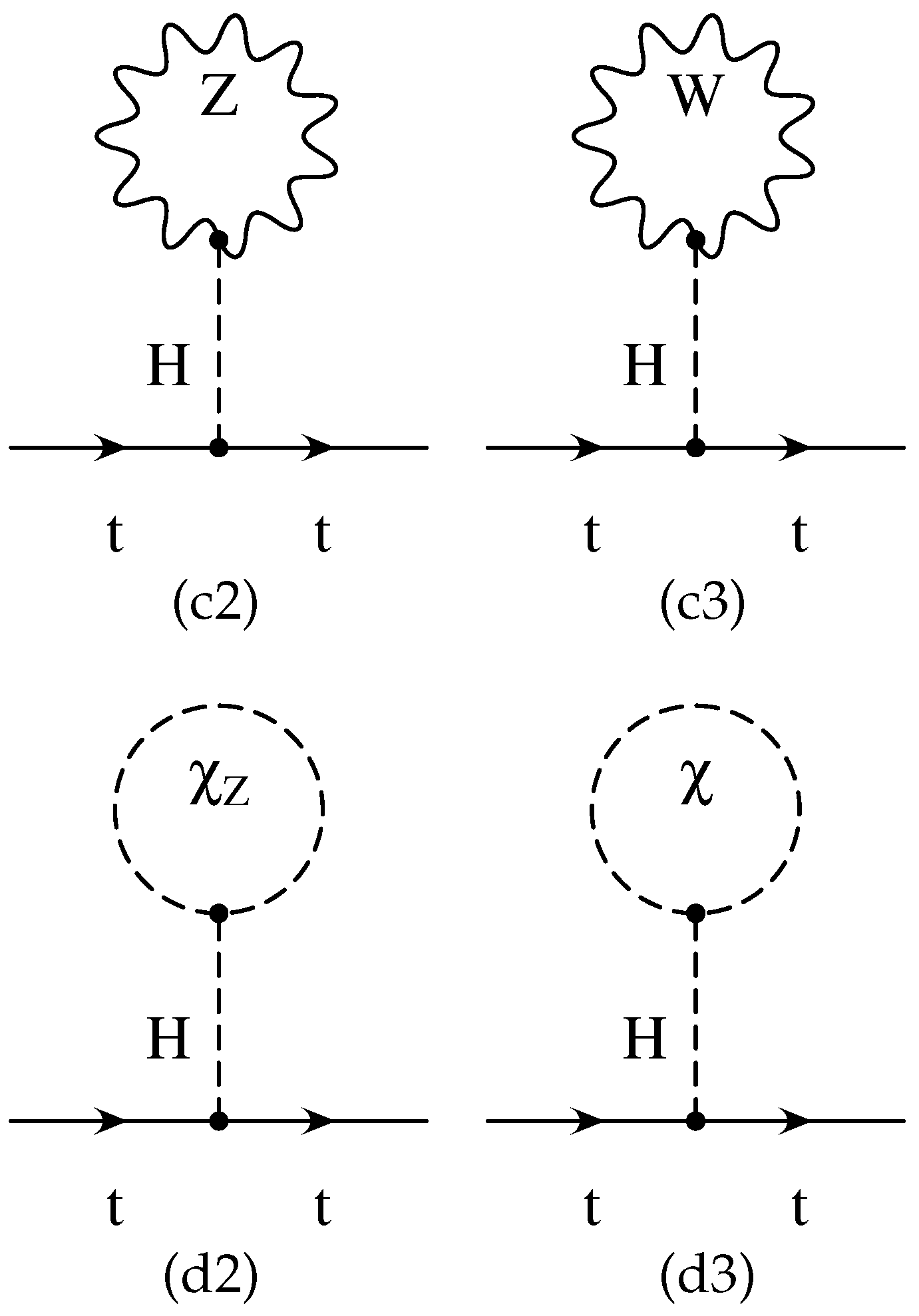
one realises that the difference does not vanish. However, as the difference is proportional to the one-point function , one might think of tadpole contributions to be taken into account. Tadpole corrections by vector and Goldstone bosons are shown in Figure 2.
For Feynman gauge one obtains
Note the vanishing momentum square for the tadpole tail (Higgs boson). The factor is a combinatorical factor due to the fact that the Z boson is its own antiparticle. As the Goldstone boson is absent for unitary gauge (i.e., does not propagate), the contribution (d2) is obviously the one which compensates the difference on the side of the Feynman gauge. However, once again the contribution (c2) will be different for unitary gauge where one obtains
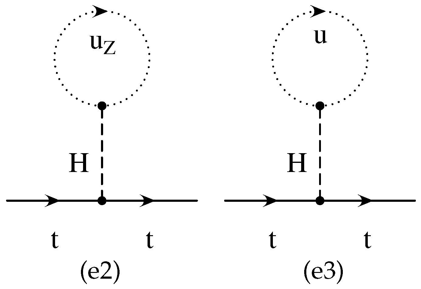
Finally, this difference will be compensated by the corresponding ghost contribution shown in Figure 3. For the tadpole with ghost loop one obtains
where the minus sign comes from the closed ghost loop. For unitary gauge () the contribution remains finite. However, the dependence on the inner momentum k disappears and, therefore, there is no ghost contribution either. On the other hand, for Feynman gauge () one obtains
Therefore, taking into account baseline vector and Goldstone corrections as well as tadpole vector, Goldstone and ghost corrections we obtain that the result for Feynman gauge is the same as the one for unitary gauge.
The situation is similar in case of the corrections by , and . However, note that in this case
Even though we take into account only the bottom quark in the loop, the sum in the loop has to run over all down-type quarks. Because of this fact and the unitarity of the Cabibbo–Kobayashi–Maskawa matrix, the factor will not appear in the final result.
6.2. The Role of Unitarity
As the parts related the two massive vector bosons Z and to the self energy of the fermion show, for the choice of unitary gauge one needs only two instead of five contributions, namely the two contributions related to the vector boson itself. Unitary gauge means , that is, the absence of the gauge fixing term. Indeed, the gauge fixing term is not necessary at all if the gauge boson carries a mass. The equation
can be solved again by the ansatz , in this case with the solution and , leading to the propoagator in unitary gauge,
7. Conclusions and Outlook
The gauge boson projector as the central tensorial object in the propagator of the vector gauge boson is closely related to the completeness relation for the polarisation vectors. A generalisation of the completeness relation to four-dimensional spacetime is proposed in a pragmatic way. Using this approach, we could identify the polarisation vectors as tetrad fields relating ordinary spacetime to polarisation spacetime (see Equation (42). While the photon projector could be expressed by mirrors on the light cone (cf. Equation (48)), the projector for massive gauge bosons turned out to be expressed in unitary gauge by default. In particular, using the example of first order fermion self energy corrections we could show that physical processes do not depend on the gauge degree of freedom.
From the different treatment of the massless photon and the massive vector bosons we can draw the conclusion that the photon might not be considered as mass zero limit of the vector boson. Indeed, at least the degree of freedoms in this limit is not continuous. This behaviour is seen also for observables related to the spin of particles, known as spin-flip effect (see e.g., References [27,28,29,30,31,32,33,34,35,36,37,38]). Fundamentally different Lie group structures for massive and massless particles were investigated in Reference [39], and the considerations in Reference [40] allow for a relation of mass and spin. Interesting enough, in combining References [39,40] a massive particle is constitued by two massless chiral non-unitary states based on the (massless) momentum vector and the light cone mirror of this, relating back to the light cone representation of the photon projector. These roughly sketched relations will be analysed in detail in a forthcoming publication.
Author Contributions
Formal analysis, P.G.; Investigation, M.N.; Methodology, S.G.; Writing of the original draft, S.G. All authors have read and agreed to the published version of the manuscript.
Funding
The research was supported by the European Regional Development Fund under Grant No. TK133, and by the Estonian Research Council under Grant No. PRG356.
Acknowledgments
We thank J. G. Körner for useful discussions on the subject of this paper.
Conflicts of Interest
The authors declare no conflict of interest.
References
- Jackson, J.D. Classical Electrodynamics, 3rd ed.; John Wiley & Sons: New York, NY, USA, 1999. [Google Scholar]
- Landau, L.; Lifshitz, E. The Classical Theory of Fields, 4th ed.; Elsevier: Amsterdam, The Netherlands, 1987. [Google Scholar]
- Greiner, W.; Reinhardt, J. Quantum Electrodynamics, 4th ed.; Springer: Berlin, Germany, 2008. [Google Scholar]
- Peskin, M.E.; Schroeder, D.V. An Introduction to Quantum Field Theory, 5th ed.; Addison-Wesley: Reading, PA, USA, 1995. [Google Scholar]
- Böhm, M.; Denner, A.; Joos, H. Gauge Theories of the Strong and Electroweak Interaction, 3rd ed.; B.G. Teubner: Stuttgart, Germany, 2001. [Google Scholar]
- Pavel, H.P.; Pervushin, V.N. Reduced phase space quantization of massive vector theory. Int. J. Mod. Phys. A 1999, 14, 2285. [Google Scholar] [CrossRef] [Green Version]
- Körner, J.G. Helicity Amplitudes and Angular Decay Distributions. In Proceedings of the Helmholtz International Summer School on Physics of Heavy Quarks and Hadrons (HQ 2013): JINR, Dubna, Russia, 15–28 July 2013; pp. 169–184. [Google Scholar]
- Berge, S.; Groote, S.; Körner, J.G.; Kaldamäe, L. Lepton-mass effects in the decays H → ZZ* → ℓ+ℓ−τ+τ− and H → WW* → ℓντντ. Phys. Rev. D 2015, 92, 033001. [Google Scholar] [CrossRef] [Green Version]
- Czarnecki, A.; Groote, S.; Körner, J.G.; Piclum, J.H. NNLO QCD corrections to the polarized top quark decay t(↑) → Xb + W+. Phys. Rev. D 2018, 97, 094008. [Google Scholar] [CrossRef] [Green Version]
- Faddeev, L.D.; Popov, V.N. Feynman Diagrams for the Yang-Mills Field. Phys. Lett. 1967, 25B, 29–30. [Google Scholar] [CrossRef]
- Lorenz, L. On the identity of the vibrations of light with electrical currents. Philos. Mag. Ser. 4 1867, 34, 287–301. [Google Scholar] [CrossRef]
- Kleinert, H. Particles and Quantum Fields; World Scientific: Singapore, 2016. [Google Scholar]
- Dirac, P.A.M. The Principles of Quantum Mechanics, 3rd ed.; Oxford University Press: Oxford, UK, 1947. [Google Scholar]
- Leibbrandt, G. Introduction to Noncovariant Gauges. Rev. Mod. Phys. 1987, 59, 1067. [Google Scholar] [CrossRef] [Green Version]
- Fermi, E. Quantum Theory of Radiation. Rev. Mod. Phys. 1932, 4, 87. [Google Scholar] [CrossRef]
- Dirac, P.A.M. Lectures in Quantum Field Theory; Academic Press: New York, NY, USA, 1966. [Google Scholar]
- Heisenberg, W.; Pauli, W. Zur Quantentheorie der Wellenfelder. Teil II. Z. Phys. 1930, 59, 168–190. [Google Scholar] [CrossRef]
- Bleuler, K. Eine neue Methode zur Behandlung der longitudinalen und skalaren Photonen. Helv. Phys. Acta 1950, 23, 567–586. [Google Scholar]
- Gupta, S.N. Theory of longitudinal photons in quantum electrodynamics. Proc. Phys. Soc. A 1950, 63, 681. [Google Scholar] [CrossRef]
- Chisholm, J.S.R. Change of variables in quantum field theories. Nucl. Phys. 1961, 26, 469–479. [Google Scholar] [CrossRef]
- Kamefuchi, S.; O’Raifeartaigh, L.; Salam, A. Change of variables and equivalence theorems in quantum field theories. Nucl. Phys. 1961, 28, 529–549. [Google Scholar] [CrossRef]
- Salam, A.; Strathdee, J.A. Equivalent formulations of massive vector field theories. Phys. Rev. D 1970, 2, 2869–2876. [Google Scholar] [CrossRef]
- Keck, B.W.; Taylor, J.G. On the equivalence theorem for S-matrix elements. J. Phys. A 1971, 4, 291. [Google Scholar] [CrossRef]
- Kallosh, R.E.; Tyutin, I.V. The Equivalence theorem and gauge invariance in renormalizable theories. Yad. Fiz. 1973, 17, 190–209, reprinted in Sov. J. Nucl. Phys. 1973, 17, 98. [Google Scholar]
- Wu, T.T.; Wu, S.L. Comparing the Rξ gauge and the unitary gauge for the standard model: An example. Nucl. Phys. B 2017, 914, 421–445. [Google Scholar] [CrossRef]
- Gegelia, J.; Meißner, U.G. Once more on the Higgs decay into two photons. Nucl. Phys. B 2018, 934, 1–6. [Google Scholar] [CrossRef]
- Lee, T.D.; Nauenberg, M. Degenerate systems and mass singularities. Phys. Rev. 1964, 133, B1549. [Google Scholar] [CrossRef]
- Kleiss, R. Hard bremsstrahlung amplitudes for e+e- collisions with polarized beams at LEP/SLC energies. Z. Phys. 1987, C33, 433–443. [Google Scholar] [CrossRef]
- Jadach, S.; Kühn, J.H.; Stuart, R.G.; Was, Z. QCD and QED corrections to the longitudinal polarization asymmetry. Z. Phys. 1988, C38, 609–617, Erratum in 1990, C45, 528. [Google Scholar] [CrossRef] [Green Version]
- Contopanagos, H.F.; Einhorn, M.B. Is there a radiative background to the search of right-handed charged currents? Nucl. Phys. 1992, B377, 20. [Google Scholar] [CrossRef] [Green Version]
- Contopanagos, H.F.; Einhorn, M.B. Physical cnsequences of mass singularities. Phys. Lett. 1992, B277, 345–352. [Google Scholar] [CrossRef] [Green Version]
- Smilga, A.V. Quasiparadoxes of massless QED. Comments Nucl. Part. Phys. 1991, 20, 69–84. [Google Scholar]
- Falk, B.; Sehgal, L.M. Helicity flip bremsstrahlung: An equivalent particle description with applications. Phys. Lett. 1994, B325, 509–516. [Google Scholar] [CrossRef]
- Körner, J.G.; Pilaftsis, A.; Tung, M.M. One loop QCD mass effects in the production of polarized bottom and top quarks. Z. Phys. 1994, C63, 575–579. [Google Scholar] [CrossRef] [Green Version]
- Groote, S.; Körner, J.G.; Tung, M.M. Polar angle dependence of the alignment polarization of quarks produced in e+e- annihilation. Z. Phys. 1997, C74, 615–629. [Google Scholar]
- Groote, S.; Körner, J.G.; Leyva, J.A. O(αs) corrections to longitudinal spin–spin correlations in e+e− → qq. Phys. Lett. 1998, B418, 192. [Google Scholar] [CrossRef] [Green Version]
- Dittmaier, S.; Kaiser, A. Photonic and QCD radiative corrections to Higgs boson production in μ+μ− → ff. Phys. Rev. 2002, D65, 113003. [Google Scholar] [CrossRef] [Green Version]
- Groote, S.; Körner, J.G.; Leyva, J.A. O(αs) corrections to the polar angle dependence of the longitudinal spin-spin correlation asymmetry in e+e− → qq. Eur. Phys. J. C 2009, 63, 391–406, Erratum in 2014, 74, 2789. [Google Scholar] [CrossRef] [Green Version]
- Saar, R.; Groote, S. Mass, zero mass and ... nophysics. Adv. Appl. Clifford Algebras 2017, 27, 2739–2768. [Google Scholar] [CrossRef] [Green Version]
- Choi, T.; Cho, S.Y. Spin operators and representations of the Poincaré group. arXiv 2018, arXiv:1807.06425. [Google Scholar]
Figure 1.
Top quark self energy diagrams. Labels like a1 are ordinal symbols for the Feynman diagrams.
Figure 1.
Top quark self energy diagrams. Labels like a1 are ordinal symbols for the Feynman diagrams.
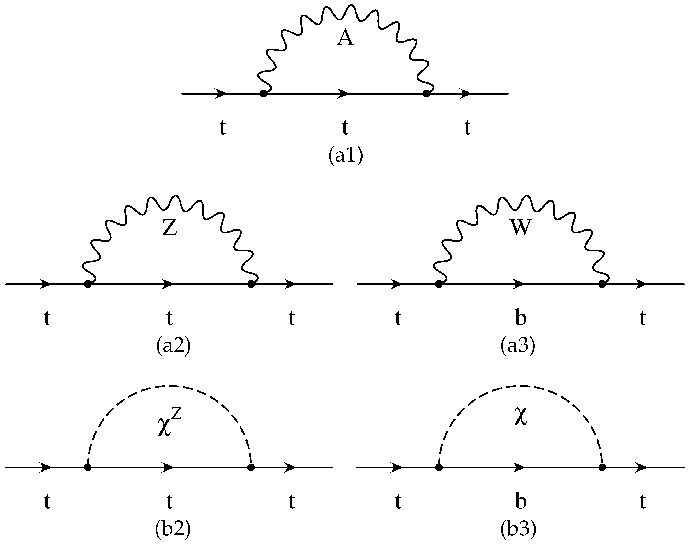
Figure 2.
Top quark self energy tadpole diagrams.

Figure 3.
Top quark self energy tadpole ghost diagrams.
© 2020 by the authors. Licensee MDPI, Basel, Switzerland. This article is an open access article distributed under the terms and conditions of the Creative Commons Attribution (CC BY) license (http://creativecommons.org/licenses/by/4.0/).
Share and Cite
MDPI and ACS Style
Gallagher, P.; Groote, S.; Naeem, M. Gauge Dependence of the Gauge Boson Projector. Particles 2020, 3, 543-561. https://doi.org/10.3390/particles3030037
AMA Style
Gallagher P, Groote S, Naeem M. Gauge Dependence of the Gauge Boson Projector. Particles. 2020; 3(3):543-561. https://doi.org/10.3390/particles3030037
Chicago/Turabian StyleGallagher, Priidik, Stefan Groote, and Maria Naeem. 2020. "Gauge Dependence of the Gauge Boson Projector" Particles 3, no. 3: 543-561. https://doi.org/10.3390/particles3030037