Article

Effects of Electrical and Electromechanical Parameters on Performance of Galloping-Based Wind Energy Harvester with Piezoelectric and Electromagnetic Transductions

1
College of Mechatronic Engineering, Qiqihar University, Qiqihar 161006, China
2
School of Mechanical and Mechatronic Engineering, University of Technology Sydney, Ultimo, NSW 2007, Australia
3
Department of Mechanical Engineering, University of Auckland, Auckland 1010, New Zealand
*
Author to whom correspondence should be addressed.
Vibration 2019, 2(2), 222-239; https://doi.org/10.3390/vibration2020014
Submission received: 9 April 2019 / Revised: 8 June 2019 / Accepted: 18 June 2019 / Published: 20 June 2019

Abstract

:
This paper presents an analysis of galloping-based wind energy harvesters with piezoelectric and electromagnetic transductions. The lumped parameter models of the galloping-based piezoelectric energy harvester (GPEH) and galloping-based electromagnetic energy harvester (GEMEH) are developed and the approximate analytical solutions of the equations are derived using the harmonic balance method (HBM). The accuracy of the approximate analytical solutions is validated by the numerical solutions. A parametric study is then conducted based on the validated models and solutions to understand the effects of the dimensionless load resistance, r, and electromechanical coupling strength (EMCS) on various quantities indicating the performance of the harvesters, including the dimensionless oscillating frequency, cut-in wind speed, displacement, and average power output. The results show that both r and EMCS can affect the dimensionless oscillating frequencies of the GPEH and GEMEH in a narrow frequency range around the natural frequency. A significant decrease in the displacement around r = 1 for GEPH and at a low r for GEMEH indicates the damping effect induced by the increase in EMCS. There are two optimal r to achieve the maximal power output for GPEH given strong EMCS while there is only one optimal r for GEMEH. Both GPEH and GEMEH show similar characteristics in that the optimal power outputs can reach saturation with an increase of the EMCS. The findings from the parametric study provide useful guidelines for the design of galloping-based energy harvesters with different energy conversion mechanisms.

1. Introduction

In recent years, the field of energy harvesting has received significant research interest due to the quest to exploit renewable energy sources. The objective of energy harvesting is to convert ambient energy sources into usable electrical energy to operate small electronic devices, such as wireless sensors [1], health monitoring sensors [2], and medical implants [3]. A number of ambient energy sources have been recognized to be promising for energy harvesting, including sunlight, wind, ocean wave, thermal gradient, and mechanical vibration. Among them, wind energy is a kind of ubiquitous energy source existing in outdoor and indoor environments, such as the natural wind outside a room and the wind flow in ventilation and air conditioning ducts inside the room. Large scale wind turbines have been developed to generate high power output in strong wind conditions. It is impractical to shrink the size of wind turbines to harvest small wind energy due to higher manufacturing costs and lower energy harvesting efficiency. One promising solution is to utilize wind flow-induced aerodynamic instability (such as galloping [4,5], flutter [6,7], and vortex-induced vibration [8]) to extract vibration energy. The extracted energy from an vibration-based energy harvesting system can be converted into electricity using piezoelectric or electromagnetic means [9].
Transverse galloping is a fluid-elastic instability that appears in some elastic bluff bodies when the velocity of the incident flow exceeds a critical value [10]. Earlier efforts focused on how the angle of the attack and Reynolds number affect the behavior of galloping [10,11]. Some studies also investigated the effect of the geometry of the cross-section of the bluff body on the amplitude of the structure [12]. In recent years, the transverse galloping phenomenon induced by wind flow has attracted increasing research interest from the field of energy harvesting. Many researchers have studied the effect of various geometries of cross-sections of the bluff bodies on energy harvesting performance [13,14,15,16,17,18], where square [14], triangular [15], rectangular [16], and D-section [17] sections are available in the literature. Theoretical and experimental methods are adopted to evaluate the dynamic response of the harvesters and their electrical outputs. Available theoretical models include the lumped parameter model [14], the single- and multi-mode distributed-parameter models [19], and the equivalent circuit model [20], where the galloping force is modeled by a quasi-steady approximation [11]. Abdelkefi et al. [21] theoretically studied the effect of the cross-section geometry (square, triangle, and D-section) on the onset speed of galloping and the level of the output power. Using a linear form, it was demonstrated that the isosceles triangle with δ = 30° and square cross-sections are the best-sections to harvest energy at low freestream velocities. Using the nonlinear normal form, it demonstrated that, for small wind speeds, the isosceles triangle with a δ = 30° cross-section is the best cross-section for enhancing the level of harvested power. In an experimental case study, Yang et al. [22] compared the electrical outputs of the GPEH with different cross-section geometries (square, triangular, rectangle, and D-shape) and concluded that the square cross-section geometry is superior to other cross-section geometries. Many studies have investigated the effect of the load resistance on the performance of the GPEH and GEMEH with a resistive circuit [21,22,23,24]. Some other researchers focus on the galloping-based energy harvester with a sophisticated circuit. Tan et al. [25] studied the intrinsic effect of inductance and load resistance on the performance of a GPEH with a resistive-inductive circuit. Zhao et al. [26] derived the explicit output responses of a GPEH with the sophisticated interface circuits by using the energy balance method. The optimal load and coupling were calculated for maximum power generation. In terms of the influence of electrical and electromechanical parameters, some attention has been given to GPEHs while very little attention has been given to GEMEHs. A comprehensive understanding on the influence of these parameters on galloping-based harvesters with different energy transduction mechanisms is important and thus worthy of further investigation.
The motivation of this paper is to conduct a comprehensive analysis of the effect of electrical and electromechanical parameters on the performance of both the GPEH and GEMEH. Lumped parameter models are established for the GPEH and GEMEH and the approximate analytical solutions of the equations for the GPEH and GEMEH are derived using the HBM. The accuracy of the approximate analytical solutions is validated by the numerical solutions. Parametric studies are performed to investigate the effects of the load resistance and EMCS on the dimensionless oscillating frequency, cut-in wind speed, displacement, and average power output for the GPEH and GEMEH based on the validated models and the approximate analytical solutions. The effect of the EMCS on the optimal average power outputs of the GPEH and GEMEH is also investigated.

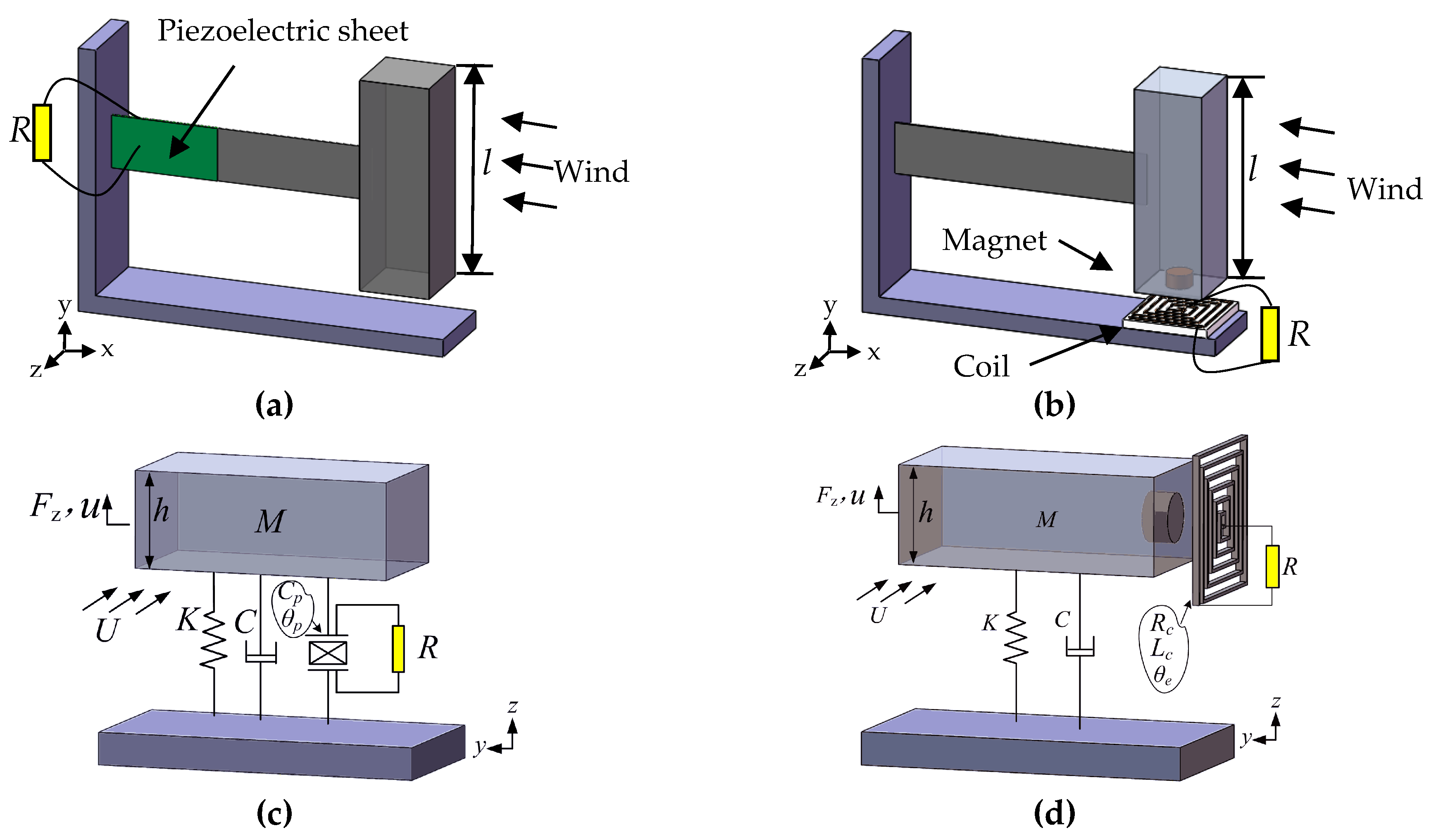
2. Configurations of GPEH and GEMEH

Figure 1a,b show a GPEH and GEMEH, respectively. Both have a similar mechanical structure, i.e., a cantilever beam with a tip bluff body at the free end. The bluff body has a square cross-section with the length of l and the frontal dimension of h facing the wind flow. The bluff body can oscillate in the direction normal to the wind flow when the wind speed, U, exceeds a critical value. In Figure 1a, a piezoelectric sheet is bonded to the cantilevered beam, which can convert the vibration into electricity due to the mechanical strain of the beam induced by the oscillation of the bluff body. In Figure 1b, a magnet is installed inside the bluff body approaching the side of the planar fixed coil. The oscillation of the bluff body with the magnet can induce current generated in the planar coil due to the motion of the magnet relative to the coil. Figure 1c,d show the simplified lumped parameter models for the GPEH and GEMEH, respectively. The mechanical structure of the harvester is simplified as a similar single degree of freedom (SDOF) model, which consists of the mass of the bluff body, M; spring stiffness, K; and damping, C. In Figure 1c, the piezoelectric element with the capacitance, Cp, and the electromechanical coupling coefficient, θp, is inserted between the base and the mass, M, for piezoelectric energy harvesting. In Figure 1d, an electromagnetic member with the coil resistance, Rc, the inductance, Lc, and the electromechanical coupling coefficient, θe, is used for electromagnetic energy harvesting. In Figure 1c,d, Fz is the aerodynamic force acting on the bluff body, which is induced by the wind flow; u is the deflection of the bluff body in the z direction; and R is the load resistance.

3. Numerical Model

3.1. GPEH

The single-mode lumped parameter model of a GPEH is often written as [20]:
M u ¨ + C u ˙ + K u + θ p V = F z = 1 2 ρ h L U 2 [ A 1 ( u ˙ U + β u ) + A 3 ( u ˙ U + β u ) 3 ] ,
θ p u ˙ + C p V ˙ + V / R = 0 ,
where (·) = / t ; V is the voltage across the load resistor, R; ρ is the air density; A1 and A3 are the empirical coefficients using polynomial fitting for the aerodynamic force [22]; and β is the coefficient relating the transverse displacement and the rotational angle at the free end of the cantilevered beam.
The state space vector is defined as:
X = { x 1 x 2 x 3 } = { u u ˙ V }
We can write the governing equations of the GPEH in the state space form as:
X ˙ = { x ˙ 1 x ˙ 2 x ˙ 3 } = { x 2 C M x 2 K M x 1 θ p M x 3 + ρ h L U 2 2 M [ A 1 ( x 2 U + β x 1 ) + A 3 ( x 2 U + β x 1 ) 3 ] θ p C p x 2 1 R C p x 3 }
The numerical solution can be obtained by numerically solving Equation (4) using ODE45 in MATLAB.

3.2. GEMEH

The governing equation of a GEMEH can be written as:
M u ¨ + C u ˙ + K u + θ e I = F z = 1 2 ρ h L U 2 [ A 1 ( u ˙ U + β u ) + A 3 ( u ˙ U + β u ) 3 ]
θ e u ˙ + L c I ˙ + ( R c + R ) I = 0 ,
where I is the current through the load resistor, R.
Due to the small inductance (using a printed spiral planar microcoil based on micromaching technology) and low frequency, the internal impedance caused by the coil inductance is much less than the internal resistance and is thus negligible [27,28,29]. Rearranging Equation (6), we can express the current as:
I = θ e R c + R u ˙ .
Substituting Equation (7) into Equation (5) gives:
M u ¨ + ( C + θ e 2 R c + R ) u ˙ + K u = 1 2 ρ h L U 2 [ A 1 ( u ˙ U + β u ) + A 3 ( u ˙ U + β u ) 3 ] .
The state space vector is defined as:
X = { x 1 x 2 } = { u u ˙ }
We can write the governing equation of the GEMEH in the state space form as:
X ˙ = { x ˙ 1 x ˙ 2 } = { x 2 K M x 1 1 M ( C + θ e 2 R c + R ) x 2 + ρ h L U 2 2 M [ A 1 ( x 2 U + β x 1 ) + A 3 ( x 2 U + β x 1 ) 3 ] } .

4. Approximate Analytical Solution

In this section, HBM is used to find the approximate solutions of the governing equations of the GPEH and GEMEH.

4.1. GPEH

It is assumed that the higher order harmonics are negligible and the steady state solution of Equations (1) and (2) is in the form as:
u = u m cos ω t ,   V = V m cos ( ω t + φ ) ,
where um and Vm are the amplitude of the displacement and the voltage, respectively; ω is the oscillating frequency, which is near but not always exactly the same as the natural frequency of the GPEH, since the aerodynamics can cause a change of the stiffness of the system; and φ is the phase difference between V and u.
Substituting the solutions given in Equation (11) into Equations (1) and (2), expanding the terms and then omitting higher-order terms, and after balancing the first-order harmonic terms, sinωt, cosωt, a set of the first order approximate differential equations can be obtained:
K u m M u m ω 2 + θ p V m cos φ 1 2 ρ h L U 2 ( A 1 β u m + 1 4 A 3 3 β u m 3 ω 2 U 2 + 3 4 A 3 β 3 u m 3 ) = 0 ,
( 1 2 ρ h L U 2 ( A 1 U + 3 4 A 3 u m 2 ω 2 U 3 + 1 4 A 3 3 β 2 u m 2 U ) C ) u m ω θ p V m sin φ = 0 ,
C p V m ω cos φ + V m R sin φ = θ p u m ω ,
C p V m ω sin φ V m R cos φ = 0 .
Four unknowns, ϕ, um, Vm, and ω, can be solved from the set of algebraic equations given in Equations (12)–(15). Firstly, from Equation (15), the phase difference can be determined to take the following form:
tan φ = 1 R C p ω .
Hence, we have:
sin φ = 1 1 + ( R C p ω ) 2 ,   cos φ = R C p ω 1 + ( R C p ω ) 2 .
After squaring Equations (14) and (15) and adding them together, and after rearranging, the following relationship between Vm and um is obtained as:
V m = θ p R ω 1 + ( R C p ω ) 2 u m .
In order to ease the analysis, we introduced the following dimensionless parameters as:
ω n = K M , k p 2 = θ p 2 K C p , ζ = C 2 K M , Ω = ω ω n , r = R C p ω n , M ^ = M ρ h 2 L , U ^ = U ω n h ,
where ωn is the natural angular frequency of the galloping-based harvester, and ωn = 2πfn, where fn is the short circuit fundamental frequency of the harvester.
Substituting the first term in Equation (17) and Equation (18) into Equation (13), and using the dimensionless parameters given in Equation (19), the explicit expression of the displacement can be obtained as:
u m = [ ζ + k p 2 r 2 ( 1 + r 2 Ω 2 ) 1 4 U ^ M ^ A 1 ] 3 16 U ^ M ^ A 3 ( Ω 2 U ^ 2 h 2 + β 2 ) .
Rewriting Equation (20) in a dimensionless form yields:
u ^ m = u m h = [ ζ + k p 2 r 2 ( 1 + r 2 Ω 2 ) 1 4 U ^ M ^ A 1 ] 3 16 U ^ M ^ A 3 ( Ω 2 U ^ 2 + β 2 h 2 ) .
For Equation (18), using the dimensionless expression, u ^ m = u m / h , and the terms given in Equation (19), the relationship between Vm and u ^ m is obtained as:
V m = K h θ p k p 2 r Ω 1 + r 2 Ω 2 u ^ m .
The average power at steady state is then expressed as:
P a v e = V m 2 2 R = ω n K h 2 k p 2 r Ω 2 2 ( 1 + r 2 Ω 2 ) u ^ m 2 .
By rewriting Equations (22) and (23) and introducing the expression of u ^ m given in Equation (21), the dimensionless voltage can be obtained as:
V ^ m = V m K h θ p = k p 2 r Ω 1 + r 2 Ω 2 [ ζ + k p 2 r 2 ( 1 + r 2 Ω 2 ) 1 4 U ^ M ^ A 1 ] 3 16 U ^ M ^ A 3 ( Ω 2 U ^ 2 + β 2 h 2 )
The dimensionless average power is:
P ^ a v e = P a v e ω n K h 2 = k p 2 r Ω 2 2 ( 1 + r 2 Ω 2 ) ζ + k p 2 r 2 ( 1 + r 2 Ω 2 ) 1 4 U ^ M ^ A 1 3 16 U ^ M ^ A 3 ( Ω 2 U ^ 2 + β 2 h 2 )
By substituting the second term in Equation (17) and Equation (20) into Equation (12), then introducing dimensionless parameters given in Equation (19), and after rearrangement, the following is obtained:
1 Ω 2 + k p 2 r 2 Ω 2 1 + r 2 Ω 2 β h U ^ ( 2 ζ + k p 2 r 1 + r 2 Ω 2 ) = 0 ,
from which the explicit expression of the dimensionless oscillating frequency, Ω, is obtained as:
Ω = ( 1 + k p 2 2 β h U ^ ζ ) r 2 1 + ( ( 1 + k p 2 2 β h U ^ ζ ) r 2 1 ) 2 + 4 r 2 ( 1 2 β h U ^ ζ β h U ^ k p 2 r ) 2 r 2 .
For short circuit (R = 0) and open circuit (R → ∞) conditions at U = 0, Equation (27) can be expressed as:
Ω s c = 1 , Ω o c = 1 + k p 2 ,
where Ωsc and Ωoc are dimensionless short circuit and open circuit frequencies, respectively.
When the wind speed, U, is nonzero, from Equation (27), two dimensionless frequencies for short circuit and open circuit conditions can be obtained as:
Ω s c = 1 2 ζ U ^ β h ,   Ω o c = 1 + k p 2 2 ζ U ^ β h .
For the bluff body with the square section, the empirical aerodynamic coefficients, A3, is negative [22]. To ensure a real root of Equation (20), we have:
ζ + k p 2 r 2 ( 1 + r 2 Ω 2 ) 1 4 U ^ M ^ A 1 0 .
The dimensionless cut-in wind speed of the GPEH can thus be expressed as:
U ^ c r = M ^ A 1 ( 4 ζ + 2 k p 2 r 1 + r 2 Ω 2 ) ,
where the empirical aerodynamic coefficient, A1, must be positive.
The results in Equations (20)–(31) agree well with the derivation based on the energy balance method [26].

4.2. GEMEH

By substituting the first term given in Equation (11) into Equation (8) and expanding the terms, and after balancing the first-order harmonic terms, sinωt and cosωt, and omitting the higher-order terms, a set of the first order approximate differential equations can be obtained:
K u m M u m ω 2 1 2 ρ h L U 2 ( A 1 β u m + 1 4 A 3 3 β u m 3 ω 2 U 2 + 3 4 A 3 β 3 u m 3 ) = 0 ,
( 1 2 ρ h L U 2 ( A 1 U + 1 4 A 3 3 β 2 u m 2 U + 3 4 A 3 u m 2 ω 2 U 3 ) ( C + θ e 2 R c + R ) ) u m ω = 0 .
Solving ω and um from Equations (32) and (33), we have:
ω = K ( C + θ e 2 R c + R ) U β M ,
and:
u m = C + θ e 2 R c + R 1 2 ρ h L U A 1 3 8 ρ h L A 3 ( ω + β 2 U ) ,
The following dimensionless parameters are introduced as:
ω n = K M ,   k e 2 = θ e 2 M ω n R c ,   ζ = C 2 K M ,   r = R R c ,   M ^ = M ρ h 2 L ,   U ^ = U ω n h .
By substituting the terms given in Equation (36) into Equation (34), the explicit expression of the frequency, ω, can be obtained as:
ω = ω n 1 ( 2 ζ + k e 2 1 + r ) U ^ β h .
By rewriting Equation (37), the dimensionless oscillating frequency is obtained as:
Ω = ω ω n = 1 ( 2 ζ + k e 2 1 + r ) U ^ β h .
When the wind speed, U = 0, the frequency is:
Ω = 1 .
When the wind speed, U, is nonzero, the dimensionless oscillating frequency for short circuit (R = 0) and open circuit (R → ∞) conditions are given, respectively, as:
Ω s c = 1 ( 2 ζ + k e 2 ) U ^ β h ,   Ω o c = 1 2 ζ U ^ β h .
For Equation (35), by substituting Equation (34) into Equation (35) and then using the dimensionless parameters given in Equation (36), after rearrangements, we have:
u m = ζ + k e 2 2 ( 1 + r ) 1 4 U ^ M ^ A 1 3 16 U ^ M ^ A 3 ( 1 U ^ 2 h 2 2 ζ β U ^ h k e 2 U ^ h ( 1 + r ) β + β 2 ) .
Dimensionless displacement yields:
u ^ m = u m h = ζ + k e 2 2 ( 1 + r ) 1 4 U ^ M ^ A 1 3 16 U ^ M ^ A 3 ( 1 U ^ 2 2 ζ U ^ β h k e 2 U ^ ( 1 + r ) β h + β 2 h 2 ) .
By introducing the current expression given in Equation (7) and the time derivative of the displacement expression given in Equation (11), the instantaneous power on R can be calculated as:
P = I 2 R = ( θ e R c + R u ˙ ) 2 R = θ e 2 ( R c + R ) 2 ω 2 u m 2 ( 1 cos 2 ω t ) 2 R .
After ignoring the high-order harmonics (cos2ωt) in Equation (43), and then inserting the expressions of ω given in Equation (37) into Equation (43), and introducing the dimensionless parameters given in Equation (36), the average power is given as:
P a v e = θ e 2 ( R c + R ) 2 ω 2 u m 2 R 2 = ω n K h 2 k e 2 r ( 1 + r ) 2 [ 1 2 ( ζ + k e 2 2 ( 1 + r ) ) U ^ β h ] u ^ m 2 .
The dimensionless average power is:
P ^ a v e = P a v e ω n K h 2 = k e 2 r ( 1 + r ) 2 [ 1 2 ( ζ + k e 2 2 ( 1 + r ) ) U ^ β h ] u ^ m 2 .
Since A3 < 0 for the square-sectioned bluff body, according to Equations (35) and (41), to ensure a real root of Equation (41), we have:
ζ + k e 2 2 ( 1 + r ) 1 4 U ^ M ^ A 1 0 .
Thus, the dimensionless cut-in wind speed of the GEMEH can be calculated as:
U ^ c r = M ^ A 1 ( 4 ζ + 2 k e 2 1 + r ) .

5. Results

In this work, the physical and empirical parameters of the GPEH were from [26]. The parameters used in the following calculations are listed in Table 1. For the GPEH, the capacitance of the piezoelectric element was Cp = 25.7 nF. For the GEMEH, the internal resistance of the spiral planar coils was assumed as Rc = 10 Ω. The other parameters were made the same for both the GPEH and GEMEH.

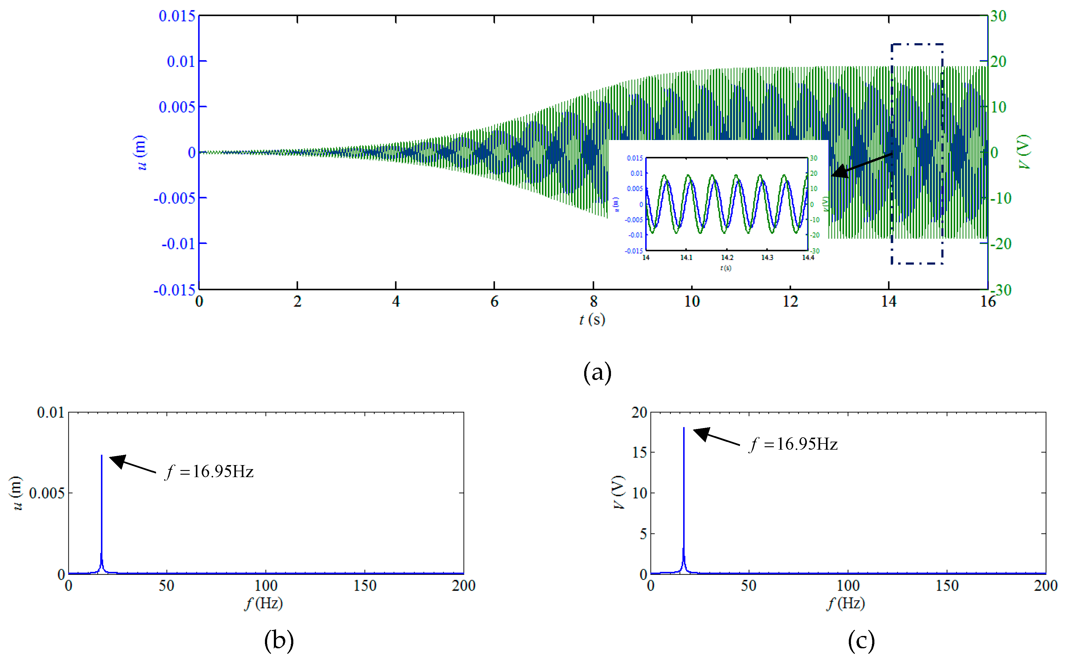
5.1. Validation of Approximate Analytical Solution

5.1.1. GPEH

Figure 2a–c show the time responses of u and V of the GPEH with R = 365.4 kΩ, θp = 0.00009 N/V, and U = 4 m·s−1 (corresponding to r = 1, k p 2 = 0.01, U ^ = 1.878) and their frequency spectra of the steady state. The time responses were obtained from the numerical simulation by MATLAB. In Figure 2b,c, it clearly shows that the dominant frequency of u and V is the fundamental frequency of the GPEH. The results indicate the feasibility of using the single harmonic approximation (Equation (11)) as the steady state solution of Equations (1) and (2).
Figure 3a–c show the dimensionless average power of the GPEH from the approximate analytical solutions of the HBM over a range of dimensionless load resistances, r, for various piezoelectric EMCS, k p 2 , at the dimensionless wind speed, U ^ , of 1.878, 2.817, and 3.756 (corresponding to 4 m·s−1, 5 m·s−1, and 6 m·s−1, respectively). It can be seen from Figure 3a–c that for a weak EMCS, k p 2 = 0.01, the system gallops throughout the dimensionless load resistance range from 0.01 to 100. The maximal P ^ a v e appears at the point, r = 1. With the increase of EMCS, k p 2 = 0.04 or 0.09, the behavior of galloping is significantly affected by the load resistance. When U ^ = 1.878 (Figure 3a), for both k p 2 = 0.04 and 0.09, galloping ceases in a range of points around r = 1 and two optimal powers appear on both sides of r = 1. The optimal powers have the same amount, but the range of the ceasing of galloping for k p 2 = 0.09 is wider than that for k p 2 = 0.04. When U ^ = 2.817 (Figure 3b), a small valley appears at r = 1 for k p 2 = 0.04. For k p 2 = 0.09, the optimal powers are the same as those for k p 2 = 0.04 and the range of the ceasing of galloping shrinks as compared to the lower wind speed of U ^ = 1.878. When U ^ = 3.756 (Figure 3c), the GPEH can gallop with all r and a deep valley appears at r = 1 for k p 2 = 0.09 with two optimal powers on both sides. Figure 3d–f show the power curves of the GPEH with various wind speeds from the numerical simulation using MATLAB. Good agreement between the approximate analytical solution using the HBM and the numerical solution can be observed.

5.1.2. GEMEH

Figure 4a,b show the time response of the displacement and its frequency spectrum at the steady state for the GEMEH with R = 10 Ω, θe = 0.172 N/A, and U = 4 m·s−1 (corresponding to r = 1, k e 2 = 0.01, U ^ = 1.878). Similar to the GPEH, it is shown in Figure 4b that the dominant frequency in the response is the fundamental frequency of the GEMEH.
Figure 5a–c show the dimensionless average power of the GEMEH from the approximate analytical solutions using the HBM over a range of dimensionless load resistances, r, for various electromagnetic EMCS, k e 2 , at the dimensionless wind speeds of 1.878, 2.817, and 3.756 (corresponding to 4 m·s−1, 5 m·s−1, and 6 m·s−1, respectively). It can be seen from Figure 5a–c that when k e 2 = 0.01, the harvester gallops throughout the dimensionless load resistance range of r from 0.01 to 100 for three different wind speed conditions. An increase in the wind speed can obtain improved power peaks. When U ^ = 1.878, for k e 2 = 0.04, galloping ceases in the range of low r. For k e 2 = 0.09, galloping disappears in a wider range of r than that for k e 2 = 0.04 and the peak power shifts to the higher r. It means that a higher k e 2 needs to match a higher r for galloping. When U ^ = 2.817 and 3.756, Figure 5b,c show the similar trends as Figure 5a, but with increased maximal dimensionless power outputs. Figure 5d–f show the power curves of the GEMEH with various wind speeds based on the numerical simulation using MATLAB. The same trends and almost the same power outputs from the numerical solution validate the approximate analytical solution using the HBM.

5.2. Parametric Study on Load Resistance and EMCS

Based on the validated models and their approximate analytical solutions using HBM, in this section, a parametric study was performed to investigate the effects of varying r and EMCS on different quantities indicating the dynamic response and energy harvesting performance of the GPEH and GEMEH. The quantities include Ω, U ^ c r , u ^ m , and P ^ a v e .

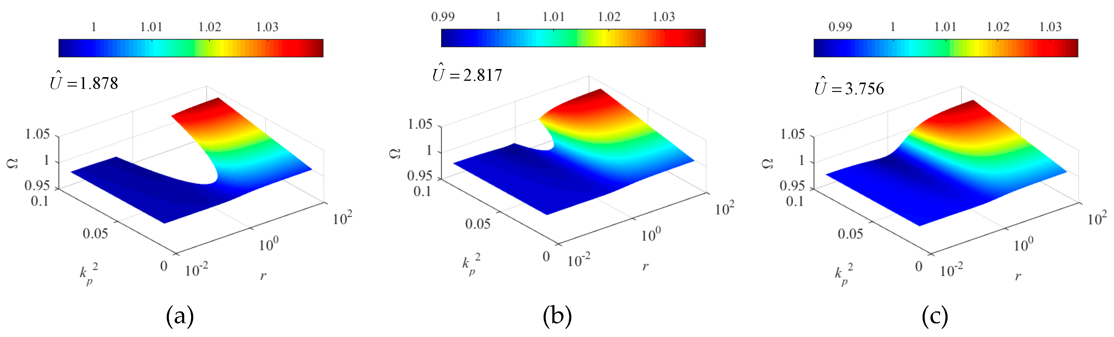
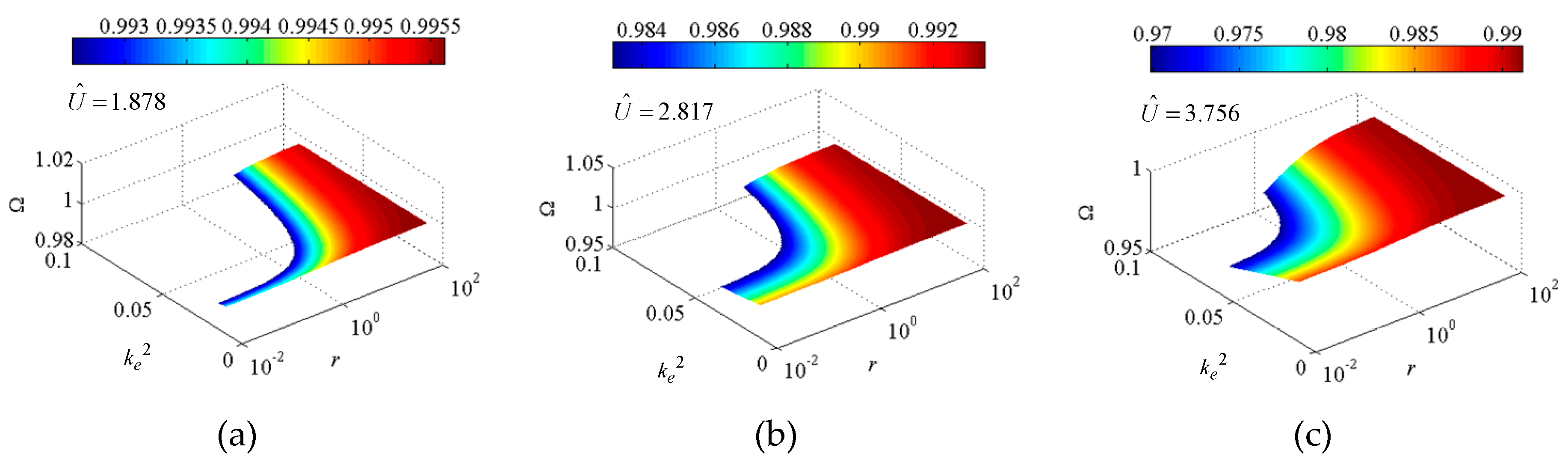
5.2.1. Effects on Dimensionless Oscillating Frequency Ω

Figure 6a–c show 3D plots of the dimensionless oscillating frequency, Ω, of the GPEH with a range of k p 2 and r, for three U ^ of 1.878, 2.817, and 3.756, respectively. r is given from 0.01 to 100. k e 2 is given from 0.01 to 0.09. The region with no data indicates that galloping does not occur with the given k p 2 and r. It can be seen from Figure 6a–c that when U ^ = 1.878, the ceasing of galloping starts from k p 2 = 0.031 around r = 1. The region of the ceasing of galloping expands with the increase of k p 2 . When U ^ = 2.817, the ceasing of the galloping starts from k p 2 = 0.0686 around r = 1. When U ^ = 3.756, the harvester gallops in the entire given ranges of k p 2 and r. In addition, it can be observed from each graph that in the galloping region with r ≤ 1, the increase of r and k p 2 can lead to minor changes of Ω. While for r > 1, the increase of r and k p 2 could significantly increase Ω. This analysis indicates that the oscillating frequencies of the GPEHs are not always equal to their own natural frequencies. The difference is due to the effect of r and EMCS.
Figure 7a–c show 3D plots of the dimensionless oscillating frequency, Ω, of the GEMEH with a range of k e 2 and r, for three U ^ of 1.878, 2.817, and 3.756, respectively. It can be seen from Figure 7a–c that when U ^ = 1.878, galloping ceases for a high k e 2 and a small r. With an increase of U ^ from 1.878 to 2.817 and further to 3.756, the region for the ceasing of galloping shrinks. In addition, it can seen from each graph that in the regions where galloping occurs, with a given k e 2 , an increase of r can induce the increase of Ω. With a given r, an increase of k e 2 can cause the decrease of Ω. It is noted that Ω is close to, but a bit less than 1. It means that the GEMEH oscillates around their own natural frequencies, but with a small difference due to the effect of r and EMCS.

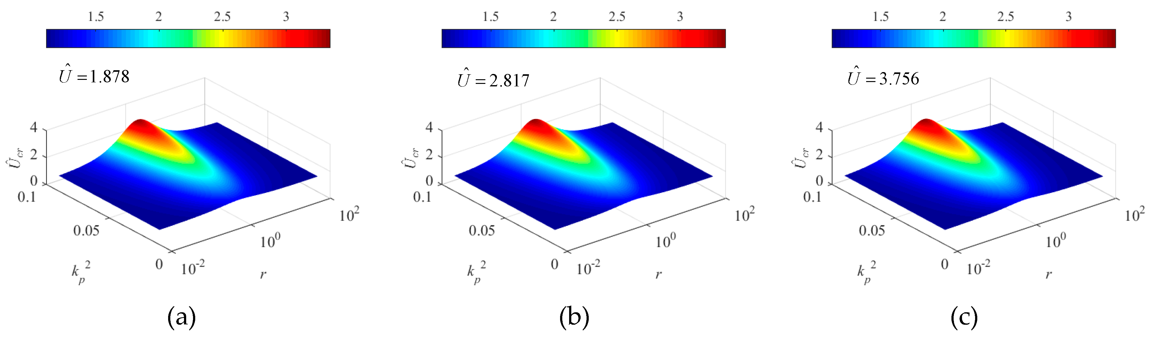
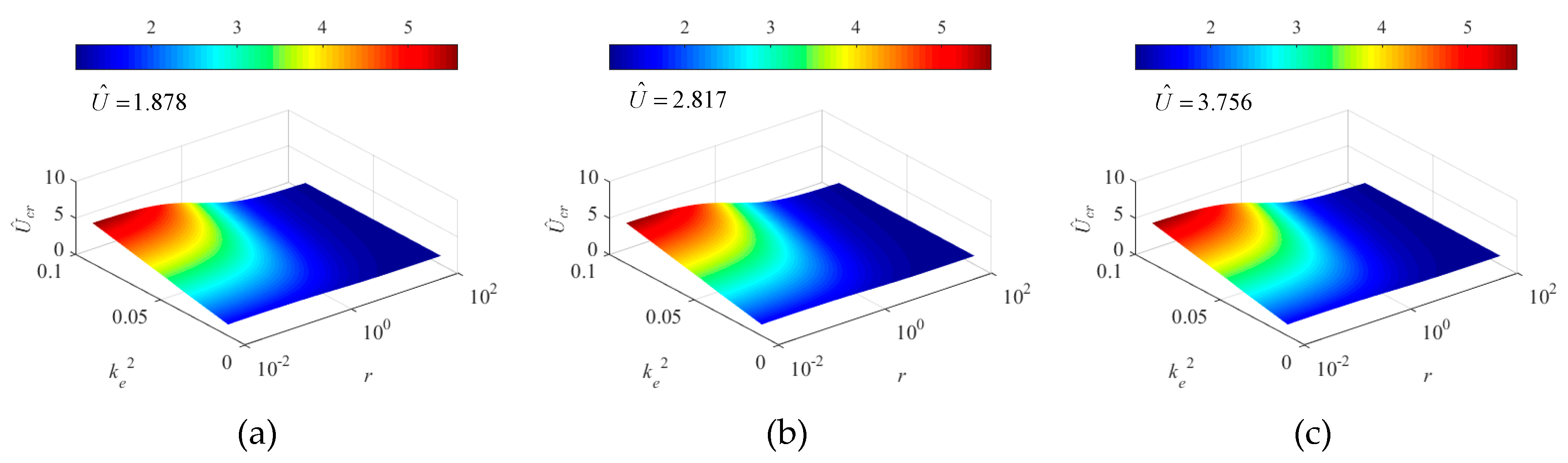
5.2.2. Effects on Dimensionless Cut-In Wind Speed, U ^ c r

Figure 8a–c show 3D plots of the dimensionless cut-in wind speed, U ^ c r , of the GPEH with a range of k p 2 and r, for three U ^ of 1.878, 2.817, and 3.756, respectively. It can be seen from Figure 8a–c that all three graphs are identical, which means the dimensionless wind speed, U ^ , has no impact on U ^ c r . It can also be observed from each graph that for a given k p 2 , the maximal U ^ c r appears at r = 1. For a given r around 1, an increase of k p 2 can induce the increase of U ^ c r . It thus implies that the higher k p 2 makes it more difficult for galloping to occur. That is the reason of the appearance of the region of the ceasing of galloping for higher k p 2 and around r = 1 (Figure 6a,b). In addition, since U ^ c r does not change with U ^ , it is no surprise that this region will shrink and disappear with the increase of U ^ (Figure 6).
Figure 9a–c show 3D plots of the dimensionless cut-in wind speed, U ^ c r , of the GEMEH with a range of k e 2 and r, for three U ^ of 1.878, 2.817, and 3.756, respectively. It can be seen from Figure 9a–c that for GEMEH, U ^ has no impact on U ^ c r . It can be observed from each graph that both the decrease of r and the increase of k e 2 lead to the increase in U ^ c r . This explains the reason that galloping ceased in the region with higher k e 2 and lower r in Figure 7. In addition, similar to the GPEH, since U ^ c r does not change with U ^ , it is no surprise that this region will shrink and disappear with the increase of U ^ (Figure 7).

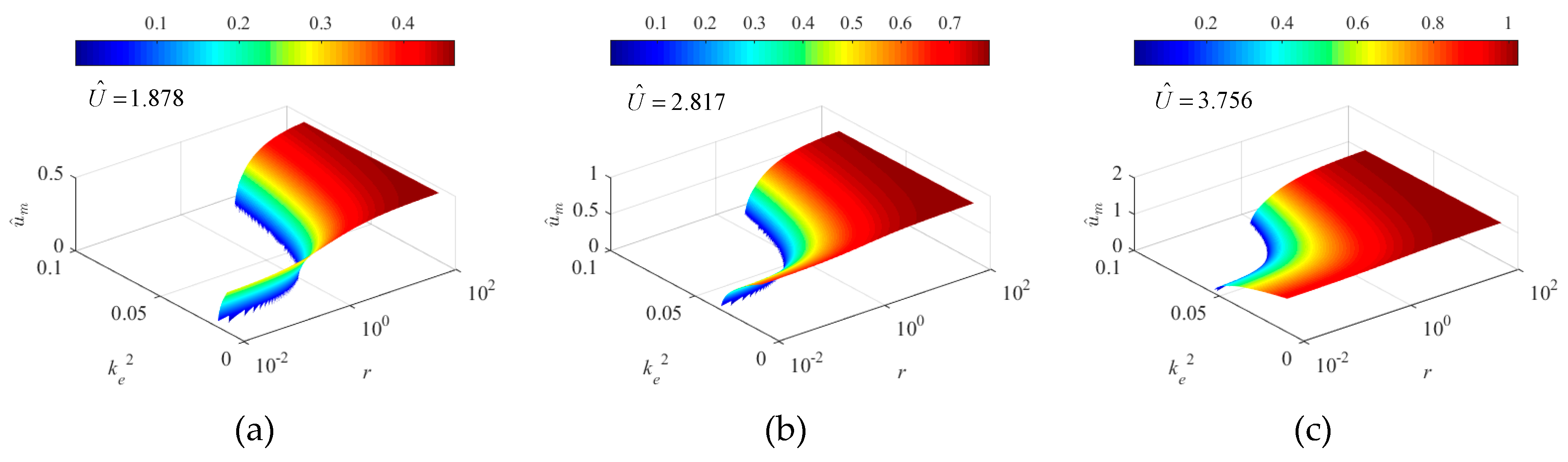
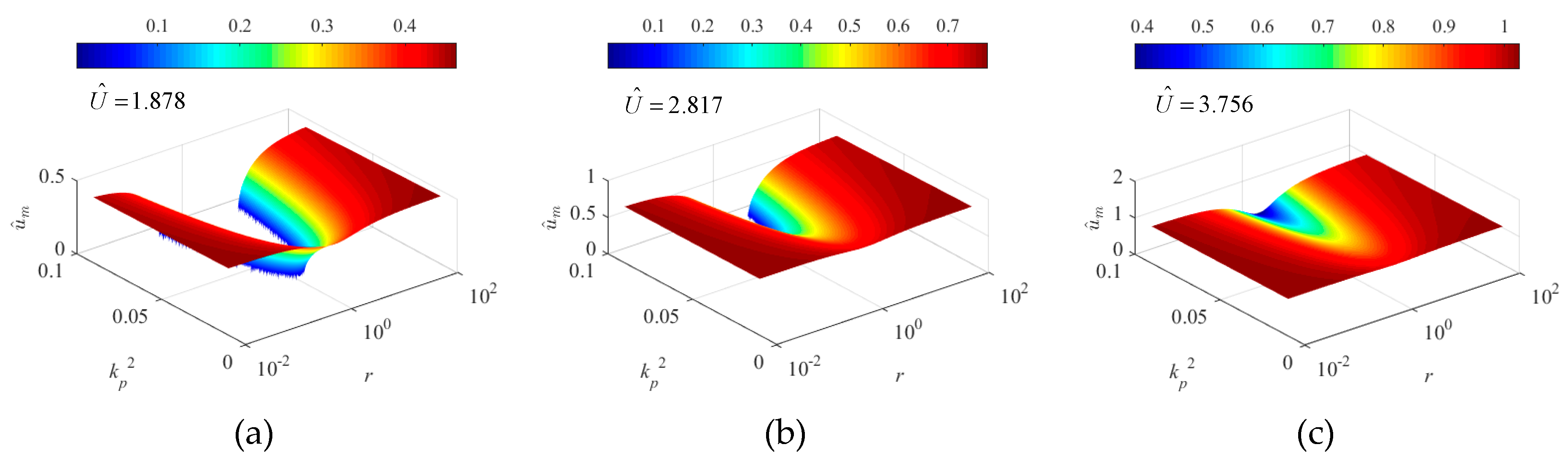
5.2.3. Effects on Dimensionless Displacement, u ^ m

Figure 10a–c show 3D plots of the dimensionless displacement, u ^ m , of the GPEH with a range of k p 2 and r, for three U ^ of 1.878, 2.817, and 3.756, respectively. It can be seen from Figure 10a–c that when U ^ increases from 1.878 to 3.756, the maximal u ^ m increases from nearly 0.5 to nearly 1. A valley is visible in each graph, where an increase in k p 2 can lead to the increase of the width of valley around r = 1. For a given r around 1, the increase of k p 2 can lead to a significant decrease of u ^ m and even zero displacement in some regions (galloping ceases for a low U ^ ). It indicates that k p 2 has a damping effect especially for r around 1. This effect is more pronounced under a low wind speed condition.
Figure 11a–c show 3D plots of the dimensionless displacement, u ^ m , of the GEMEH with a range of k e 2 and r, for three U ^ of 1.878, 2.817, and 3.756, respectively. It can be seen from Figure 11a–c that when U ^ increases from 1.878 to 3.756, the maximal u ^ m increases from nearly 0.5 to nearly 1. There are regions of zero displacement in low r and high k e 2 in each graph, where galloping ceases for a low U ^ . In the galloping region, with a given low r, the minor increase of k e 2 can lead to a significant decrease of u ^ m . It implies that k e 2 has a damping effect especially for low r. Similar to the GPEH, this effect is more pronounced under a low wind speed condition.

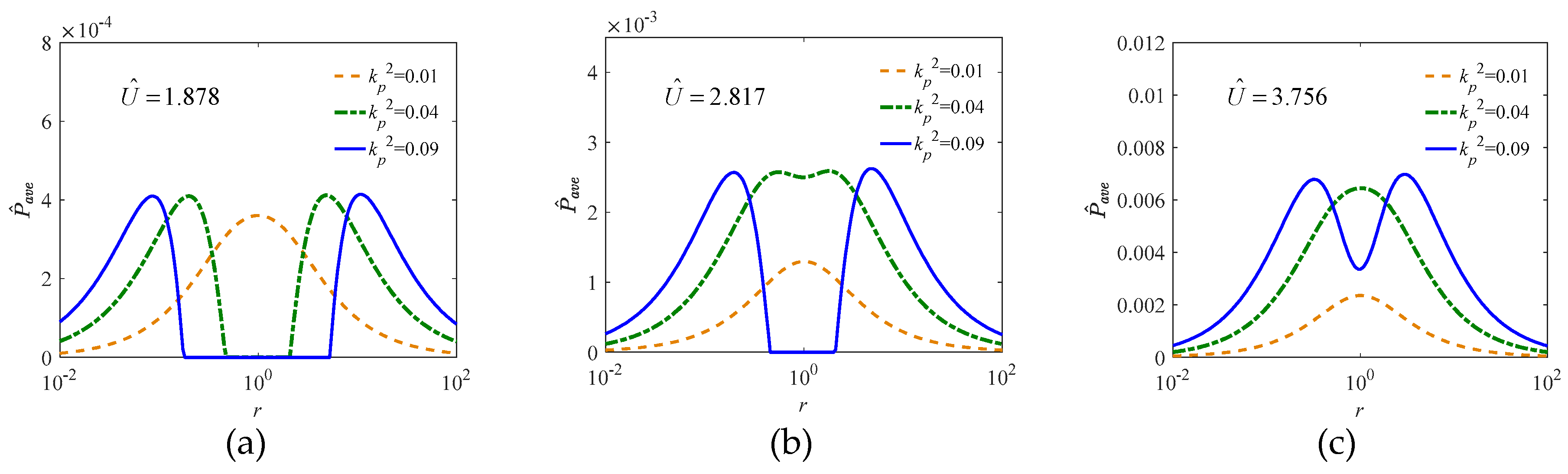
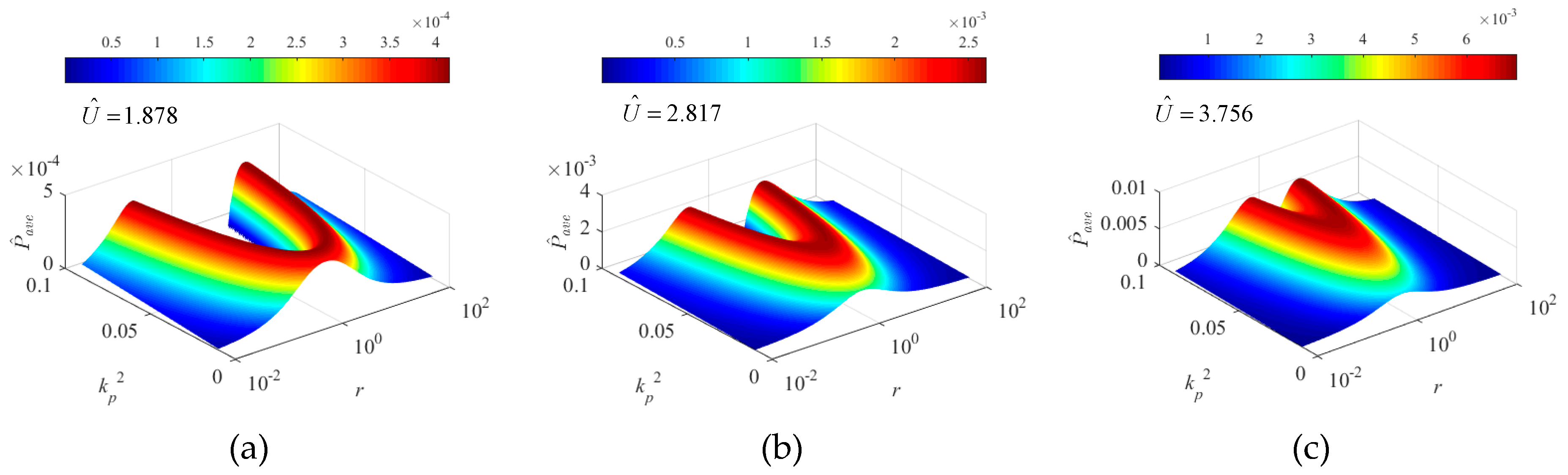
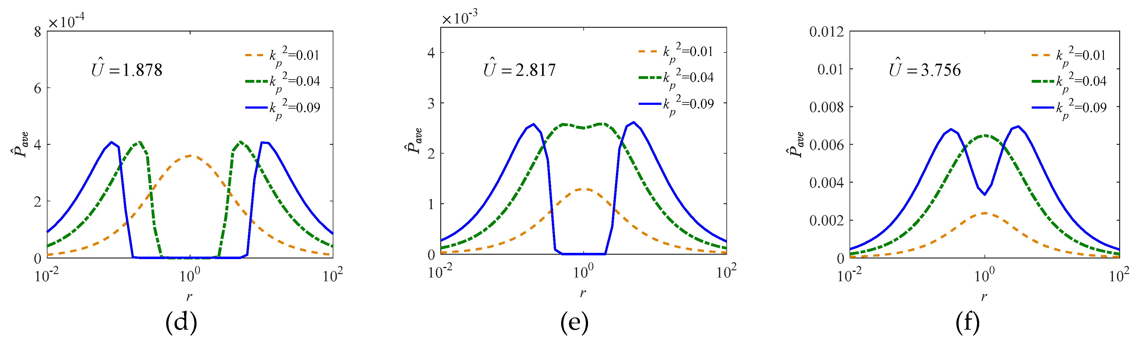
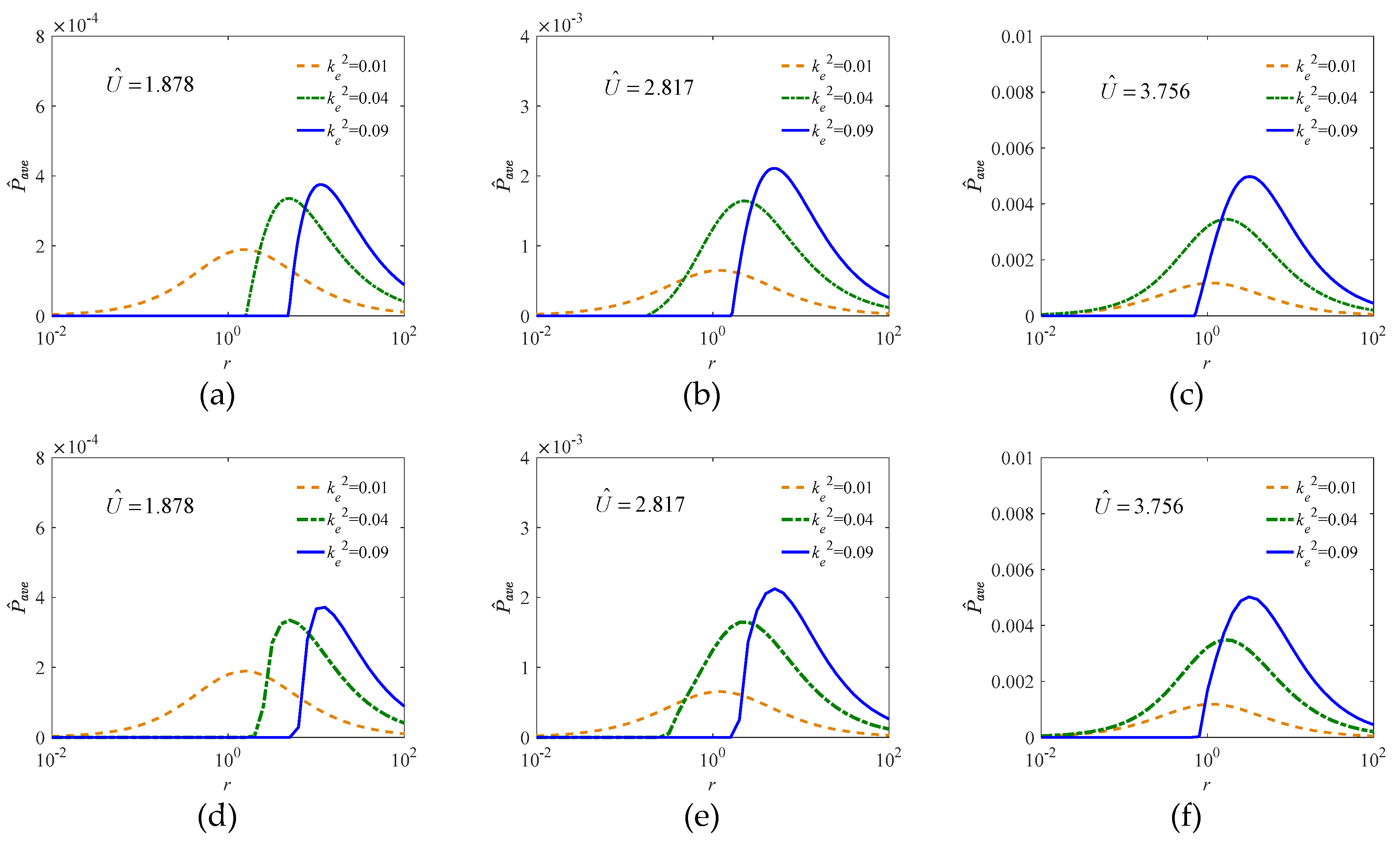
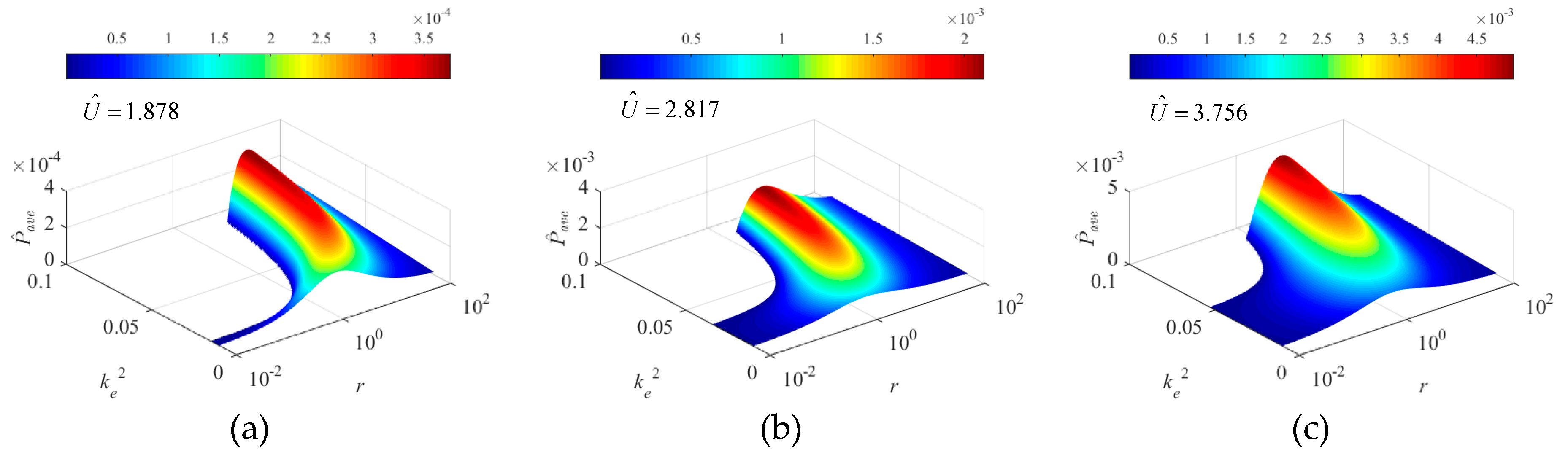
5.2.4. Effects on Dimensionless Power, P ^ a v e

Figure 12a–c show the 3D plots of the dimensionless average power, P ^ a v e , of the GPEH with a range of k p 2 and r, for three U ^ of 1.878, 2.817, and 3.756, respectively. It can be seen from Figure 12a–c that with an increase of k p 2 from 0.01 to 0.09, P ^ a v e increases, saturates, and then forms two power ranges, which have an equal height and branch from r around 1, and a valley between the ranges. Thus, for a small k p 2 , there only exists an optimal r around 1 to achieve the maximal power output. While, for a large k p 2 , there exists two optimal r to achieve the maximal power output. For a low U ^ = 1.878 or 2.817, the power output could reduce to zero in the valley since galloping ceases. An increase in U ^ can increase galloping regions.
Figure 13a–c show 3D plots of the dimensionless average power, P ^ a v e , of the GEMEH with a range of k p 2 and r, for three U ^ of 1.878, 2.817, and 3.756, respectively. It can be seen from Figure 13a–c that with an increase of k e 2 from 0.01 to 0.09, the power peak increases, saturates gradually, and forms a power range on the side of r > 1. Thus, for a given k e 2 , there exists an optimal r to achieve the maximal power output. In each graph, there are regions of zero power in low r and high k e 2 since galloping ceases. An increase in U ^ can enlarge the galloping regions induced by r and k e 2 .

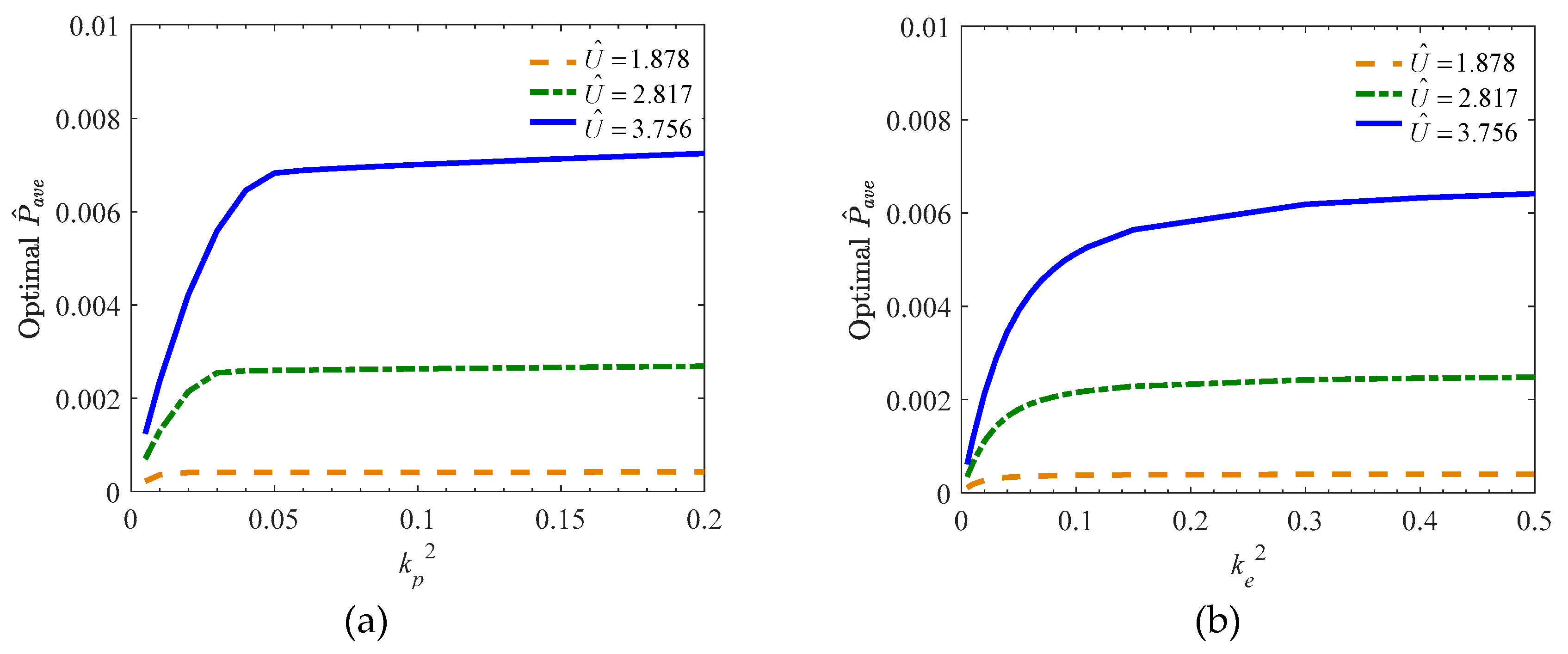
5.2.5. Optimal Power Outputs

Figure 14a,b plot the envelopes of the optimal P ^ a v e versus k p 2 and k e 2 for the GPEH and GEMEH, respectively. It can be seen from Figure 14a that with a given U ^ , with the increase of k p 2 , the optimal P ^ a v e increases rapidly and then barely changes with k p 2 . With an increase in U ^ , the critical k p 2 at which P ^ a v e saturates increases. The curves for the GEMEH (Figure 14b) show similar trends to the GPEH (Figure 14a).

6. Conclusions

In this work, we investigated the performance of two types of galloping-based wind energy harvesters with two different energy conversion mechanisms, namely, the piezoelectric effect (i.e., GPEH) and electromagnetic induction (i.e., GEMEH). The lumped parameter models were established and the approximate analytical solutions of the equations were derived using the HBM. These solutions were validated by the numerical simulation. The effect of r and EMCS on Ω, U ^ c r , u ^ m , and P ^ a v e was investigated for the GPEH and GEMEH based on the validated models and their approximate analytical solutions. The results showed that r and EMCS can affect Ω in a narrow frequency range around 1. For the GPEH, Ω was close to 1. For the GEMEH, Ω was close, but a bit less than 1. Larger U ^ c r appeared in the region with a larger EMCS and around r = 1 for the GPEH. Larger U ^ c r appeared in the region with a larger EMCS and a smaller r for the GEMEH. A significant decrease in the displacement around r = 1 for the GEPH and at low r for the GEMEH indicated a damping effect induced by the increase of the EMCS. For the power generation of the GPEH, with a given small EMCS, one optimal r existed to achieve the maximal power output. With a given large EMCS, two optimal r existed to achieve the equal maximal power output. For the GEMEH, only one optimal r existed on the side of r > 1 to achieve the maximal power output regardless of the EMCS. Both GPEH and GEMEH showed similar characteristics in that the optimal power reached saturation with an increase of the EMCS. This parametric study provides useful guidelines in the design of galloping-based energy harvesters with different energy conversion mechanisms.

Author Contributions

Analysis and writing, H.W.; computing, L.Z.; conceptualization and methodology, L.T.

Funding

This research was supported by Heilongjiang Provincial Natural Science Foundation of China (No. LC2017028) and Fundamental Research Funds in Heilongjiang Provincial Universities of China (No. 135209229).

Conflicts of Interest

The authors declare no conflict of interest.

References

  1. Beeby, S.P.; Tudor, M.J.; White, N.M. Energy Harvesting Vibration Sources for Microsystems Applications. Meas. Sci. Technol. 2006, 17, R175–R195. [Google Scholar] [CrossRef]
  2. Yang, Z.; Zhou, S.; Zu, Z.; Inman, D. High-Performance Piezoelectric Energy Harvesters and Their Applications. Joule 2018, 2, 642–697. [Google Scholar] [CrossRef] [Green Version]
  3. Kim, D.H.; Shin, H.J.; Lee, H.; Jeong, C.K.; Park, H.; Hwang, G.-T.; Lee, H.-Y.; Joe, D.J.; Han, J.H.; Lee, S.H.; et al. In Vivo Self-Powered Wireless Transmission Using Biocompatible Flexible Energy Harvesters. Adv. Funct. Mater. 2017, 27, 1700341. [Google Scholar] [CrossRef]
  4. Elahi, H.; Eugeni, M.; Gaudenzi, P. A Review on Mechanisms for Piezoelectric-based Energy Harvesters. Energies 2018, 11, 1850. [Google Scholar] [CrossRef]
  5. Abdelkefi, A. Aeroelastic Energy Harvesting: A review. Int. J. Eng. Sci. 2016, 100, 112–135. [Google Scholar] [CrossRef]
  6. Elahi, H.; Eugeni, M.; Gaudenzi, P. Design and Performance Evaluation of a Piezoelectric Aeroelastic Energy Harvester based on the Limit Cycle Oscillation Phenomenon. Acta Astronaut. 2019, 157, 233–240. [Google Scholar] [CrossRef]
  7. Aquino, A.I.; Clautit, J.K.; Hughes, B.R. Evaluation of the Integration of the Wind-Induced Flutter Energy Harvester (WIFEH) into the Built Environment: Experimental and Numerical analysis. Appl. Energy 2017, 207, 61–77. [Google Scholar] [CrossRef]
  8. Zhang, L.; Dai, H.; Abdelkefi, A.; Wang, L. Improving the Performance of Aeroelastic Energy Harvesters by an Interference Cylinder. Appl. Phys. Lett. 2017, 111, 073904. [Google Scholar] [CrossRef]
  9. Javed, U.; Abdelkefi, A. Characteristics and Comparative Analysis of Piezoelectric-Electromagnetic Energy Harvesters from Vortex-induced Oscillations. Nonlinear Dyn. 2019. [Google Scholar] [CrossRef]
  10. Den Hartog, J.P. Mechanical Vibrations, 1st ed.; McGraw-Hill: New York, NY, USA, 1956. [Google Scholar]
  11. Naudascher, E.; Rockwell, D. Flow-Induced Vibrations: An Engineering Guide, 1st ed.; Dover Publications: New York, NY, USA, 1994. [Google Scholar]
  12. Novak, M. Aeroelastic Galloping of Prismatic Bodies. ASCE J. Eng. Mech. Div. 1969, 96, 115–142. [Google Scholar]
  13. Barrero-Gil, A.; Alonso, G.; Sanz-Andres, A. Energy Harvesting from Transverse Galloping. J. Sound Vib. 2010, 329, 2873–2883. [Google Scholar] [CrossRef]
  14. Abdelkefi, A.; Hajj, M.R.; Nayfeh, A.H. Power Harvesting from Transverse Galloping of Square Cylinder. Nonlinear Dyn. 2012, 70, 1355–1363. [Google Scholar] [CrossRef]
  15. Sirohi, J.; Mahadik, R. Piezoelectric Wind Energy Harvester for Low-power Sensors. J. Intell. Mater. Syst. Struct. 2011, 22, 2215–2228. [Google Scholar] [CrossRef]
  16. Ewere, F.; Wang, G. Performance of Galloping Piezoelectric Energy Harvesters. J. Intell. Mater. Syst. Struct. 2014, 25, 1693–1704. [Google Scholar] [CrossRef]
  17. Sirohi, J.; Mahadik, R. Harvesting Wind Energy using a Galloping Piezoelectric Beam. J. Vib. Acoust. 2011, 134, 011009. [Google Scholar] [CrossRef]
  18. Abdelkefi, A.; Yan, Z.; Hajj, M.R. Performance Analysis of Galloping-based Piezoaeroelastic Energy Harvesters with Different Cross-Section Geometries. J. Intell. Mater. Syst. Struct. 2014, 25, 246–256. [Google Scholar] [CrossRef]
  19. Zhao, L.; Tang, L.; Yang, Y. Comparison of Modeling Methods and Parametric Study for a Piezoelectric Wind Energy Harvester. Smart Mater. Struct. 2013, 22, 125003. [Google Scholar] [CrossRef]
  20. Tang, L.; Zhao, L.; Yang, Y.; Lefeuvre, E. Equivalent Circuit Representation and Analysis of Galloping-Based Wind Energy Harvesting. IEEE-ASME Trans. Mech. 2015, 20, 834–844. [Google Scholar] [CrossRef]
  21. Abdelkefi, A.; Hajj, M.R.; Nayfeh, A.H. Piezoelectric Energy Harvesting from Transverse Galloping of Bluff Bodies. Smart Mater. Struct. 2013, 22, 015014. [Google Scholar] [CrossRef]
  22. Yang, Y.; Zhao, L.; Tang, L. Comparative Study of Tip Cross-Sections for Efficient Galloping Energy Harvesting. Appl. Phys. Lett. 2013, 102, 064105. [Google Scholar] [CrossRef]
  23. Vicente-Ludlam, D.; Barrero-Gil, A.; Velazquez, A. Optimal Electromagnetic Energy Extraction from Transverse Galloping. J. Fluid. Struct. 2014, 51, 281–291. [Google Scholar] [CrossRef]
  24. Dai, H.L.; Abdelkefi, A.; Javed, U.; Wang, L. Modeling and Performance of Electromagnetic Energy Harvesting from Galloping Oscillations. Smart Mater. Struct. 2015, 24, 045012. [Google Scholar] [CrossRef]
  25. Tan, T.; Yan, Z. Electromechanical Decoupled Model for Cantilever-Beam Piezoelectric Energy Harvesters with Inductive-Resistive Circuits and Its Application in Galloping Mode. Smart Mater. Struct. 2017, 26, 035062. [Google Scholar] [CrossRef]
  26. Zhao, L.; Yang, Y. Analytical Solutions for Galloping-based Piezoelectric Energy Harvesters with Various Interfacing Circuits. Smart Mater. Struct. 2015, 24, 075023. [Google Scholar] [CrossRef]
  27. Wacharasindhu, T.; Kwon, J.W. A Micromachined Energy Harvester from a Keyboard using Combined Eectromagnetic and Piezoelectric Conversion. J. Micromech. Microeng. 2008, 18, 104016. [Google Scholar] [CrossRef]
  28. Yang, B.; Lee, C.; Xiang, W.; Xie, J.; He, J.H.; Kotlanka, R.K.; Low, S.P.; Feng, H. Electromagnetic Energy Harvesting from Vibrations of Multiple Frequencies. J. Micromech. Microeng. 2009, 19, 035001. [Google Scholar] [CrossRef]
  29. Yang, B.; Lee, C.; Kee, W.L.; Lim, S.P. Hybrid Energy Harvester based on Piezoelectric and Electromagnetic Mechanisms. J. Micro/Nanolithogr. MEMS MOEMS 2010, 9, 023002. [Google Scholar] [CrossRef]
Figure 1. (a,b) Physical models for GPEH and GEMEH; (c,d) simplified models for GPEH and GEMEH.
Vibration 02 00014 g001
Figure 2. Time response and frequency spectra of u and V for GPEH with R = 365.4 kΩ and θp = 0.00009 N/V at U = 4 m·s−1. (a) Time responses of u and V; (b) and (c) frequency spectra of u and V.
Vibration 02 00014 g002
Figure 3. Dimensionless average power output of GPEH versus r for various k p 2 at U ^ = 1.878, 2.817, and 3.756. (ac) Approximate analytical solution using HBM; (df) Numerical solution using MATLAB.
Vibration 02 00014 g003aVibration 02 00014 g003b
Figure 4. Time response and frequency spectrum of u for GEMEH with R = 10 Ω, θe = 0.172 N/A at U = 4 m·s1. (a) Time response; (b) frequency spectrum.
Vibration 02 00014 g004
Figure 5. Dimensionless average power output of GEMEH versus r for various k e 2 at U ^ = 1.878, 2.817, and 3.756. (ac) Approximate analytical solution using HBM; (df) Numerical solution using MATLAB.
Vibration 02 00014 g005
Figure 6. Three-dimensional plots of the dimensionless oscillating frequency, Ω, for GPEH with a series of k p 2 and r at: (a) U ^ = 1.878; (b) U ^ = 2.817; and (c) U ^ = 3.756.
Vibration 02 00014 g006
Figure 7. Three-dimensional plots of the dimensionless oscillating frequency, Ω, for GEMEH with a series of k e 2 and r at: (a) U ^ = 1.878; (b) U ^ = 2.817; and (c) U ^ = 3.756.
Vibration 02 00014 g007
Figure 8. Three-dimensional plots of the dimensionless cut-in wind speed, U ^ c r , for GPEH with a series of k p 2 and r at: (a) U ^ = 1.878; (b) U ^ = 2.817; and (c) U ^ = 3.756.
Vibration 02 00014 g008
Figure 9. Three-dimensional plots of the dimensionless cut-in wind speed, U ^ c r , for GEMEH with a series of k e 2 and r at: (a) U ^ = 1.878; (b) U ^ = 2.817; and (c) U ^ = 3.756.
Vibration 02 00014 g009
Figure 10. Three-dimensional plots of dimensionless displacement, u ^ m , for GPEH with a series of k p 2 and r at: (a) U ^ = 1.878; (b) U ^ = 2.817; and (c) U ^ = 3.756.
Vibration 02 00014 g010
Figure 11. Three-dimensional plots of the dimensionless displacement, u ^ m , for GEMEH with a series of k e 2 and r at: (a) U ^ = 1.878; (b) U ^ = 2.817; and (c) U ^ = 3.756.
Vibration 02 00014 g011
Figure 12. Three-dimensional plots of the dimensionless average power, P ^ a v e , for GPEH with a series of k p 2 and r at: (a) U ^ = 1.878; (b) U ^ = 2.817; and (c) U ^ = 3.756.
Vibration 02 00014 g012
Figure 13. Three-dimensional plots of the dimensionless average power, P ^ a v e , for GEMEH with a series of k e 2 and r at: (a) U ^ = 1.878; (b) U ^ = 2.817; and (c) U ^ = 3.756.
Vibration 02 00014 g013
Figure 14. Outline of the optimal dimensionless average power versus (a) k p 2 from GPEH; (b) k e 2 from GEMEH at U ^ = 1.878, 2.817, and 3.756.
Vibration 02 00014 g014
Table 1. Properties of GPEH and GEMEH.
PropertiesValuesPropertiesValues
Effective mass, M (kg)0.002783Cross section of bluff body, h × h (m)0.02 × 0.02
Effective stiffness, K (N m−1)31.5638Length of bluff body, L (m)0.1
Damping ratio, ζ0.011Fluid density, ρ (kg m−3)1.2041
Coefficient, β 10.55Aerodynamic coefficients, A1, A32.3, −18
Capacitance, Cp (nF)25.7Coil resistance, Rc (Ω)10

