

Cyclic Trends of Wildfires over Sub-Saharan Africa

1
Climate Change, Botswana Institute for Technology Research and Innovation, Private Bag 0082, Gaborone, Botswana
2
The Bradley Department of Electrical and Computer Engineering, Virginia Tech, Blacksburg, VA 24061, USA
3
Department of Environmental Science, University of Botswana, Private Bag 0704, Gaborone, Botswana
*
Author to whom correspondence should be addressed.
†
The first author was involved in the conceptualisation, data analysis, interpretation of the results, and the writing of the paper; the second author was involved in conceptualisation, the processing of satellite data, the interpretation of results, and the writing of the paper.
Fire 2023, 6(2), 71; https://doi.org/10.3390/fire6020071
Submission received: 2 December 2022
/
Revised: 2 February 2023
/
Accepted: 9 February 2023
/
Published: 16 February 2023
(This article belongs to the Special Issue Advances in Forest Fire Behaviour Modelling Using Remote Sensing)
Abstract
:In this paper, the patterns of the occurrences of fire incidents over sub-Saharan Africa are studied on the basis of satellite data. Patterns for the whole sub-Saharan Africa are contrasted with those for northern sub-Saharan Africa and southern-hemisphere Africa. This paper attempts to unravel linear trends and overriding oscillations using regression and spectral techniques. It compares fire patterns for aggregated vegetation with those for specific types, which are savannahs, grasslands, shrublands, croplands, and forests, to identify key trend drivers. The underlying cyclic trends are interpreted in light of climate change and model projections. Considering sub-Saharan Africa, northern sub-Saharan Africa, and southern-hemisphere Africa, we found declining linear trends of wildfires with overriding cyclic patterns that have a period of ∼5 years, seemingly largely driven by savannahs, grasslands, and croplands.
1. Introduction
Fire is an integral part of Earth’s biogeochemical processes and has influenced land–atmosphere interactions for more than 400 million years [1]. Fire influences many aspects of the global environment, such as the carbon cycle, atmospheric climate, and ecosystem distribution. Fire-prone ecosystems cover 40% of the land surface, and these ecosystems include major global biomes such as savannahs, grasslands, boreal forests, and shrublands. These fire-prone ecosystems are responsible for more than 85% of global fires [2,3].
Savannas are the most fire-prone ecosystems, responsible for 65% of the gross global mean fire emissions, where total global fire emissions are 8 Pg CO yr [4]. Savannahs cover about 23–33 million km, occupying 10% to 25% of Earth’s land surface [5,6,7,8,9]. Of all the world’s continents, Africa has by far the largest area of savannahs, covering about 40% to 50% (about 15 million km) of its land surface [5,10,11,12]. The largest portion of African savannahs are found in southern Africa, where they cover about 46% of the total land surface [7]. Other African savanna patches are found in East and West Africa [13]. The second largest global fraction of savannahs are in northern Australia, where they cover about 2 million km [14]. Australia’s savannahs comprise 12% of the global savannah biome, and they have some of the world’s most extensive and intact eucalyptus stands. Nearly 75% of Australia’s total burnt land area occurs in the savanna ecosystem [14]. South America has the most diverse types of savanna ecosystems, covering approximately 2.7 million km, which is about 8–10% of the global savanna biome [15,16,17,18].
The Coupled Intercomparison Project Phase 5 (CMIP5) multimodel predicted that mean annual precipitation (MAP) in arid and semiarid regions, which are part of fire-prone ecosystems, would decrease by 10–25% and 15–45% under the Representative Concentration Pathway 4.5 (RCP4.5) and RCP8.5 climatic scenarios, respectively, while mean annual temperature (MAT) would increase by 1.5–3 °C and more than 4 °C under the RCP4.5 and RCP8.5 climate scenarios, respectively, by the end of the century [IPCC 2013] [19,20,21]. Warmer and drier conditions have potential to alter biogeochemical processes such as carbon fixation and sequestration, and soil respiration [22,23]. The predicted climate change coupled with extreme weather events such as windstorms, lightning, and heat waves could enhance the accumulation of dry biomass, drier soil conditions, and increased soil surface temperature, which could, in turn, result in increased fire frequency, severity, and intensity [21,24,25,26].
In this study, we assess fire trends in sub-Saharan Africa over a period of two decades. Africa is ideal to study fire regimes and the interactions between fire and other biogeophysical processes such as vegetation and precipitation because it has the largest proportion of fire-prone biomes. The equator cuts Africa into two subcontinents with fairly different vegetation distributions owing to differences in the climate and soil patterns: the northern and southern region. The northern region (Sahel) covers the area between 10 and 20 N, stretching longitudinally from Senegal in West Africa to Sudan/Ethiopia in East Africa [27]. In this region, seasonal rainfall varies significantly in the meridional direction, but less in the zonal direction [27]. The southern region (southern Africa) is located between 10 and 35 S. The mean annual precipitation in this region increases steeply in the south–north direction [28]. This moisture gradient has resulted in a vegetation structure in which the southern portion of southern Africa is dominated by thin-leaf deciduous shrubs, while the northern part is dominated by evergreen broad-leaf trees [29]. The meridional and zonal geographical orientation of Africa’s southern and northern hemispheres, respectively, render Africa a conducive environment to study the interactions between the fire regime and environmental factors such as precipitation, vegetation structure, and land use type. Furthermore, Africa accounts for more than 50% of the total global amount of burnt vegetation annually [2,30,31,32,33,34,35].
In light of the projected climate change and associated extreme weather events, it is important to assess the fire regime in Africa under climate change. In this study, we assess African fires, looking at the burnt area for aggregated and specific vegetation types to characterise their linear trends and overriding oscillations over two decades. We hypothesize that the frequency of the oscillations might change as climate change continues to take its toll, but tracking these changes would require much longer observations than those considered in this study.
2. Materials and Methods
The study was conducted in the savannas, shrublands, croplands, forests, and grasslands of sub-Saharan Africa (SSA). The distributions of these vegetation classes over sub-Saharan Africa are shown in Figure 1. More than 50% of the surface land area in Africa is covered by savanna vegetation, which translates into more than km [7]. Southern-hemisphere Africa (SHA) has the largest continuous stretch of savannas, which cover a land surface area of approximately km, whereas northern sub-Saharan Africa (NSSA), that is, Africa north of the equator and south of the Sahara, covers about km of land surface [7,11,12,36,37]. These geographical regions are depicted in Figure 1, adopted from [37].
The Moderate Resolution Imaging Spectroradiometer (MODIS) burn product (MCD64A1 V006) was used for this analysis covering the period of 2001–2020. MCD64A1 data have a spatial resolution of 500 m and a 1-month temporal resolution. This product provides the day of the year when pixels burn [38]. The data were acquired from NASA’s Earth Observing Data and Information System (EOSDIS, https://search.earthdata.nasa.gov/search, accessed on 23 January 2022). Monthly burn products were processed following the algorithm provided in [37]. In this ensuing analysis, the key variable of consideration is the proportion of the burnt area to the total land surface. We study the trends and cyclic behaviour of this variable to detect underlying fire patterns.
2.1. Proportion of Burnt Area
Suppose that the total area of the region under consideration is A, is the area of each pixel, and the total burnt area in a year t is . Then, the proportion of the burnt area to the total land surface in year t is given by . The number of pixels in the burnt area is then given by . Therefore, the linear trend and oscillations of the proportion of burnt area are reflected in the time series for the corresponding number of pixels and vice versa. Likewise, the total number of pixels in the area under consideration is . The quantity, , changes each year according to changes in the burnt area, . If has a linear trend with gradient , then the gradient of the linear trend of (t) is . Quantity is dimensionless, whereas area has area units. On the other hand, the frequency of the oscillations of burnt area is equal to that of those for proportion .
2.2. Regression and Spectral Analysis
Consider a random variable that is drifting with time, possibly having some overriding cyclic behaviour. Realisations of this random variable may be the previously introduced . We could model the behaviour of this random variable as follows:
where is the residual (for a comprehensive discussion of linear models, see [39]) that may be a linear combination of oscillatory and random terms. Methods for fitting the linear trend are well-established, and there are relevant statistical packages that are readily available. These methods include the computations of significance values and confidence intervals for parameter estimates. In the Results section, we report parameter estimates with their corresponding estimates of significance levels.
Here, we delve into some details of spectral methods because they are rarely used in the fire community. The oscillatory term can be written as follows:
where are the Fourier coefficients, are the angular frequencies, each is the phase shift, and is the random term. The series can be written in the following alternative form:
where and . The essence of spectral analysis is to decompose a signal into components of different frequencies, and it can be traced as far back as 1974, when it was applied to economic time series [40]. It is a technique for studying cyclical or periodic behaviour. In [41], statistical tests for assessing cyclical trends in epidemiological time series were presented. To some degree, our application of spectral analysis to fire time series is novel, though the tools are well-known, especially in the mathematical sciences. Most recently, the authors in [42] presented what they called a multitaper spectral method that was a Fourier transform tailored to detect a shared frequency in a coupling among fire, vegetation, and climate.
In order to detect the oscillations of a signal, it is important to first remove the linear trend, which is a process called detrending. Detrending is a well-studied problem in econometrics, with the method of differencing being quite popular. Here, we used the method of fitting a linear trend and removing it from the data, which was chosen because of its intuitive appeal. Through detrending, a nonstationary signal can be transformed into one that is stationary. A visual inspection of a plot of the detrended signal can give a rough indication of the dominant frequencies of the signal. Better still, the Fourier analysis of the signal can reveal its fundamental and harmonic frequencies [43]. To that end, one can first compute the autocovariance of the detrended signal via
where is the time delay. Detrending yields a signal of zero mean, that is, . As an example, consider a signal that has only one angular frequency . In this case, we have
The relationship among angular frequency, , and signal frequency f is given by . Furthermore, the period and frequency of the signal are related via . If and , then the autocovariance of this signal is given by
It follows that the autocovariance function retains the frequency of the underlying signal. A visual inspection of a graph of the autocovariance function versus lead time can reveal the underlying frequency. More generally, if we have , with , we obtain
If is white noise with constant variance , then its autocovariance is given by
If we represent the periodic component of the signal as , then we can write
Taking advantage of the Cauchy–Schwartz inequality, we obtain the following result:
This helps in obtaining the bound for the autocovariance of the signal encapsulated by
where when and when . A strict equality holds if and only if the variance of the noise vanishes. The Fourier transform of , which is denoted by , is given by
In studying recurrence patterns in California wildfires, the authors in [42] applied the Fourier transform in its most basic mathematical form and not as an integral of the autocorrelation function, as presented here. The Fourier transform presented here exists provided that is square integrable, i.e., . It follows from (11) that
where is the Dirac delta function [44]. Function is the power spectrum of the signal, and its spikes correspond to the fundamental frequency and the respective harmonics.
2.3. Simulation Example
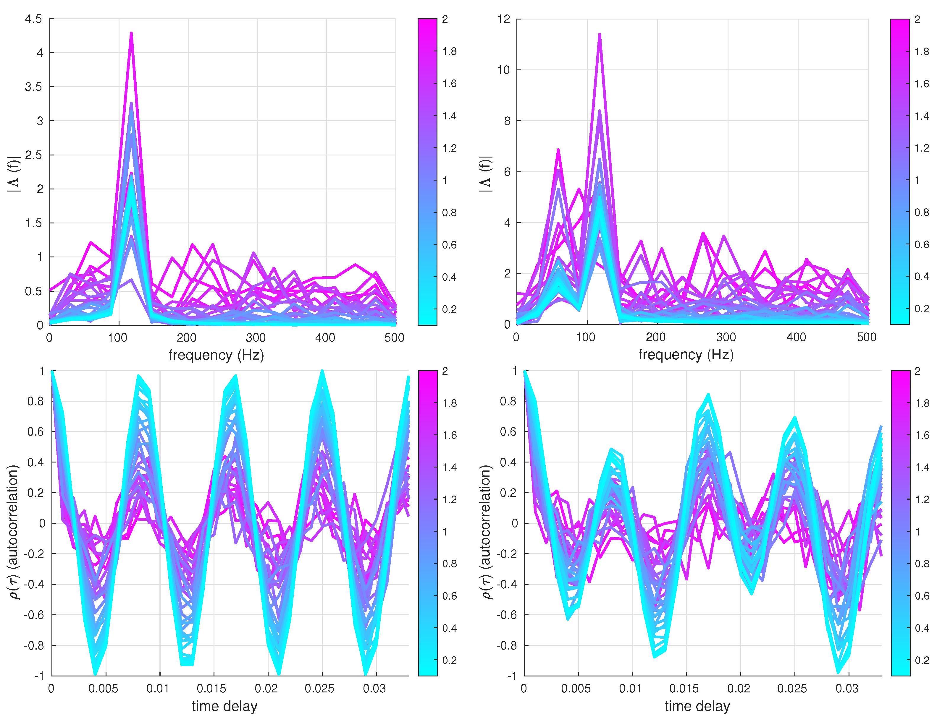
As with all natural signals, observational noise is inevitable in fire data. This was documented in [45,46], where methods for assessing noise in wildfire data were discussed, most notably the Kalman filter. In view of the presence of measurement noise in fire data, it is important to investigate how spectral analysis tools can perform in its presence. A simulation example is used to illustrate the robustness of the power spectrum and the autocorrelation function to detect underlying signal frequencies under different levels of measurement noise. The two signals are shown in Figure 2, and the corresponding power spectra and autocorrelation function graphs are shown in Figure 3. The equations for the oscillatory parts of signals on the left and right are given by, respectively,
where , , so that each signal is given by , . The noise level was selected via the scaling parameter , where is represented by the colour bar on the right of each graph. is the signal-to-noise ratio. A high value of corresponds to relatively strong measurement noise. From the graphs, it appears that the autocorrelation function was more robust to changes in the signal-to-noise ratio than the power spectrum was. This is understandable, because the power spectrum takes as input the autocorrelation function. As the signal-to-noise ratio is lowered, the power spectrum shows more false spikes, while the oscillatory nature of the autocorrelation function tends to be maintained. For a signal with a single frequency, the first peak of the autocorrelation function corresponds to the frequency of the signal. A signal that is the superposition of two signals with frequencies that are not scalar multiples of each other has the first two peaks corresponding to the two frequencies. The peaks are repeated at scalar multiples of the fundamental and harmonic frequencies. In practical situations where the frequencies are unknown a priori, it is hard to know if the additional peaks are for more underlying frequencies or just repetitions at multiples of the fundamental frequencies. The power spectrum may, therefore, have better discriminatory power because it has no inherent repetitions.
3. Numerical Results
This section presents numerical results based on the analysis of satellite data of fires over sub-Saharan Africa. Figure 4 shows graphs of a number of burns versus latitude (left) and longitude (right) as a function of time. The period of study spans two decades from 2001 to 2020. The number of burns is a simple count of the pixels in the burnt area. In the subsequent analyses, we also study the proportion of burnt area, computing both the gradient of the linear trend and the period of the underlying oscillations. The period is essentially the recurrence time of the fire oscillations/cycles. A negative gradient shows that the burnt area decreases with time, while a positive gradient shows that the burnt area increases with time.
3.1. Sub-Saharan Africa: All Vegetation
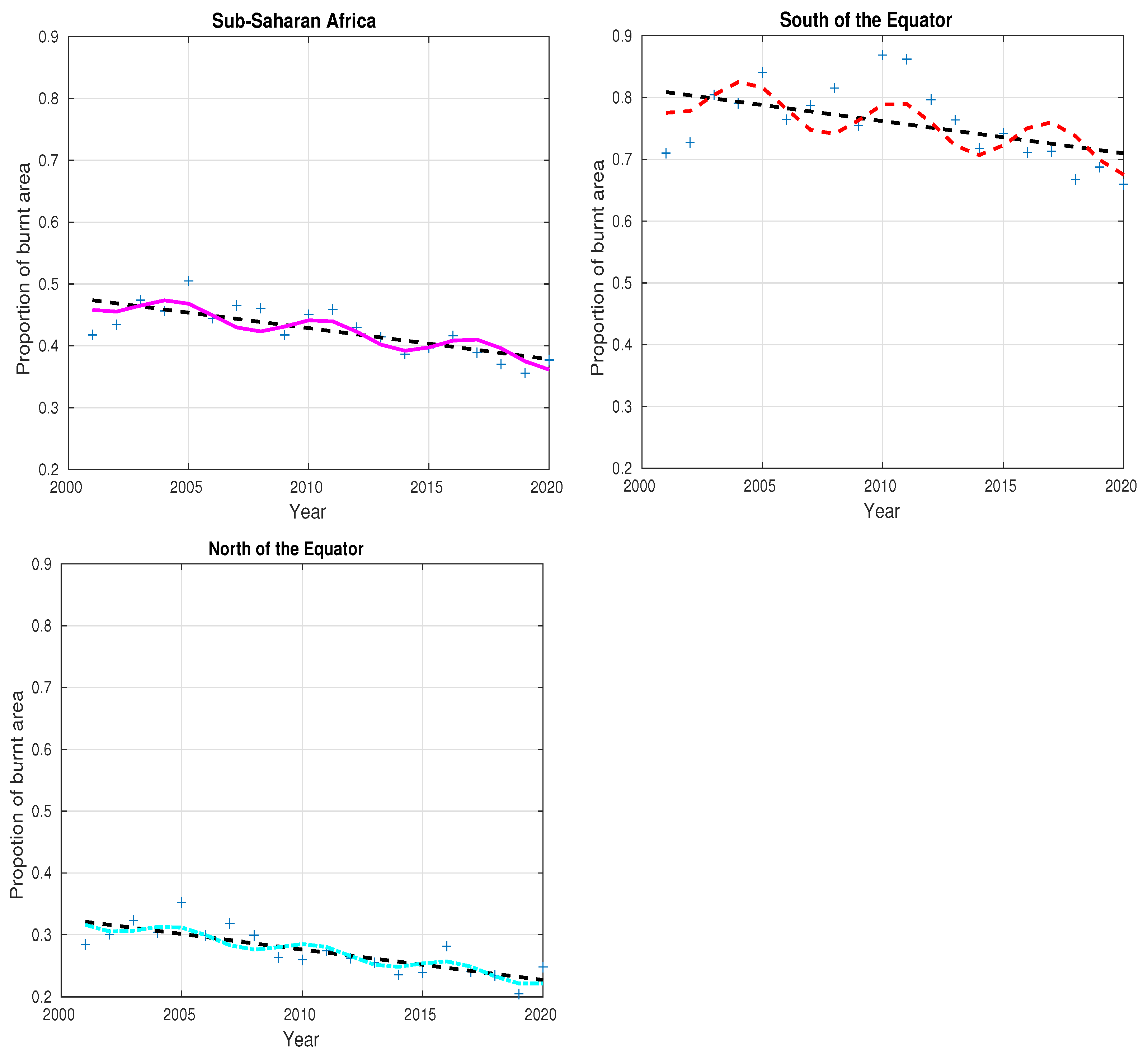
There was a trend of decreasing fires over the two decades. This trend is more pronounced on time series plots for sub-Saharan Africa, northern sub-Saharan African, and southern-hemisphere Africa, as shown in Figure 5. The blue crosses in the graphs are the actual observations. In each case, a linear trend was fitted and is depicted with a black dashed line. These graphs show the proportion of the burnt area as a function of time. The gradient for the linear trend of the sub-Saharan Africa fitting was −0.005, that for northern sub-Saharan Africa was −0.0049 and that for southern-hemisphere Africa was −0.0052. This means that the burnt area is decreasing at a rate of ∼36,000 km per annum. These were all significant at a level of 5%. In fact, the largest p-value was for southern-hemisphere Africa, 2.3%. In all three cases, it is evident that the fires have been decreasing with time over the past two decades, albeit in an oscillatory manner.
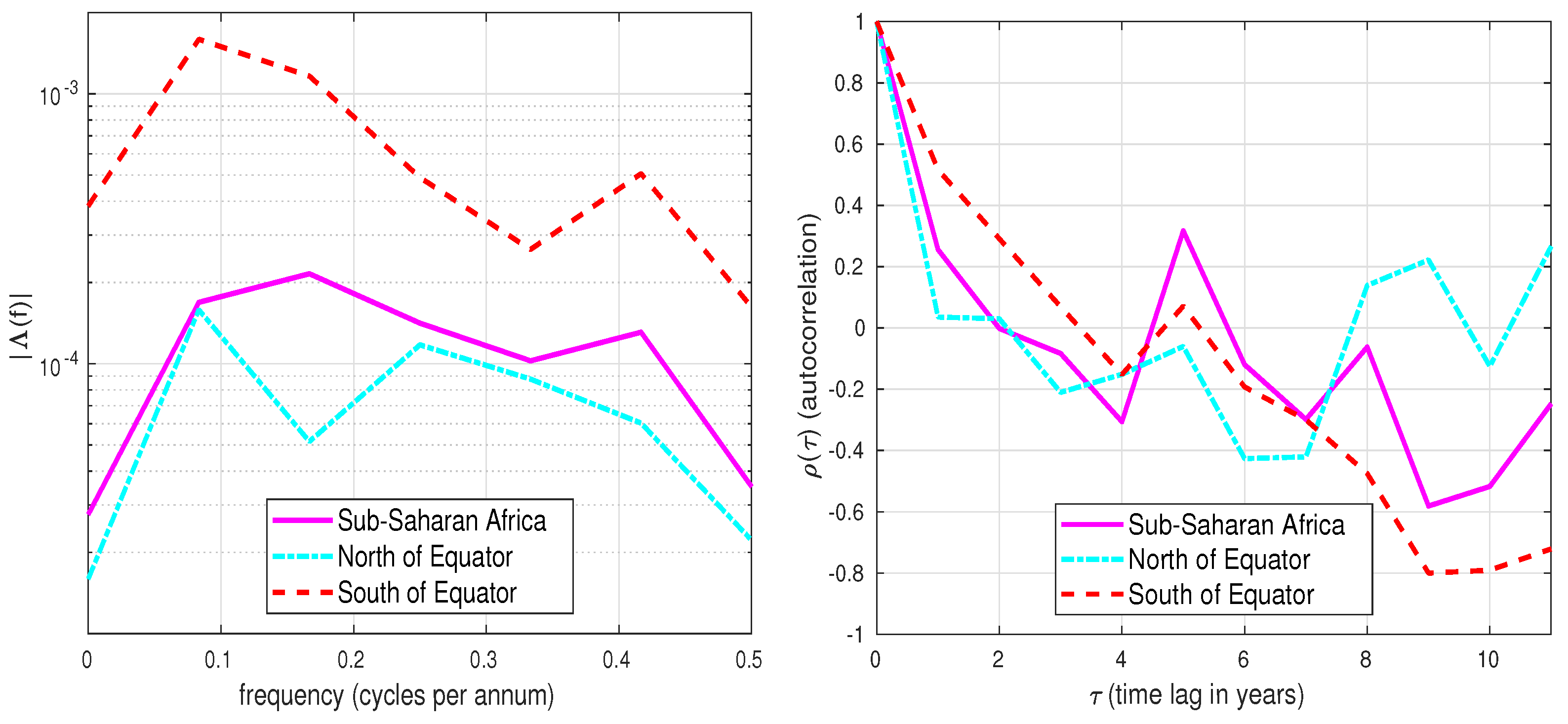
Imputing the actual nature of the oscillations is an intricate process. In order to enhance the quantification of the oscillations, it is useful to first remove the linear trend from the time series. In this study, all spectral analysis was performed after the linear trend had been removed from the original time series. The next aim was to compute the frequency (or period) of the oscillations. Graphs for the estimated trends and oscillations are shown in Figure 5, obtained by assuming that there was only one fundamental frequency (in each case) with no harmonics. Fitting more than one frequency for the particular signal length is against the principle of parsimony. The corresponding frequency was obtained via the nonlinear least-squares fitting of Equation (2). The found frequencies were for sub-Saharan Africa, northern sub-Saharan Africa, and southern-hemisphere Africa, respectively. These results are for all the fires over sub-Saharan Africa, irrespective of vegetation type. The foregoing frequencies yielded periods of years for sub-Saharan Africa, northern sub-Saharan Africa and southern-hemisphere Africa respectively. These results can be compared with those obtained from graphs of the autocorrelation as a function of time lag, shown in Figure 6. All three graphs manifested the first peak at , strongly indicating that the oscillations of the fires over the three regions of sub-Saharan Africa had periods of around 5 years. Graphs of the power spectrum showed peaks at frequencies for fires over all sub-Saharan Africa. These correspond to periods of and years. The value of was relatively close to the values obtained with nonlinear least-squares fitting and the autocorrelation function. The power spectrum for fires over northern sub-Saharan Africa yielded and , which correspond to periods of 12 and 4 years per cycle, respectively. On the other hand, the power spectrum for fires over southern-hemisphere Africa yielded peaks at and , which correspond to periods of and 2.4 years, respectively. The values obtained via the power spectrum were deemed less reliable because of the earlier indicated robustness issues. Therefore, the periods obtained via nonlinear fitting and the autocorrelation function are more reliable estimates.
3.2. All Sub-Saharan Africa: Vegetation-Specific
Next, we turn our attention to computations relating to fires based on vegetation types. The considered types were forests, savanna, shrublands, grasslands, croplands, and others, and the corresponding graphs of the autocorrelation function and power spectrum are shown in Figure 7. The coefficients of variation for the nonlinear least-squares fits for all vegetation types were all below 0.2, but a multiplicity of computational approaches gave some credence to the estimates of periods. The first considered computations were for savanna fires over all sub-Saharan Africa. On the basis of the autocorrelation function, the period of savanna fires was 5 years. The power spectrum yielded a period of years, while the least-squares nonlinear fitting yielded a period of 6.1 years. The trend gradient for savanna fires was −0.0027 with a p-value of 0.0000. This means that the burnt savanna area is decreasing at a rate of ∼26,000 km per annum. The forests yielded a trend of 0.0018 at a p-value of 0.023, while the nonlinear regression of the detrended series and power spectrum gave periods of 5.26 and 5.99 years, respectively. Thus, the burnt forest area is increasing at a rate of ∼5000 km per annum. The shrublands gave an otherwise insignificant trend of −0.0004. There were no significant periods for shrublands, with the autocorrelation function showing no noticeable peak, while the power spectrum gave 3 and 12 years. The grasslands also showed a trend of −0.0008 with a p-value of 0.1. This corresponds to a decrease in burnt area of ∼2800 km per annum. Graphs of the corresponding autocorrelation function gave periods of 2 and 8 years, while the power spectrum gave a period of 2.3 years. Nonlinear regression gave a return time of 6.1 years. Lastly, croplands showed a negative trend, while others showed no trend. Moreover, croplands yielded return times of 5 and 8 years via the autocorrelation function, while nonlinear regression gave a 6.4-year period. Other vegetation types gave a period of 4 years via the power spectrum and autocorrelation function, while nonlinear regression gave a period of 6.5 years. The linear trend for other vegetation types was zero at a significance level of 2%.
3.3. Northern Sub-Saharan Africa: Vegetation-Specific
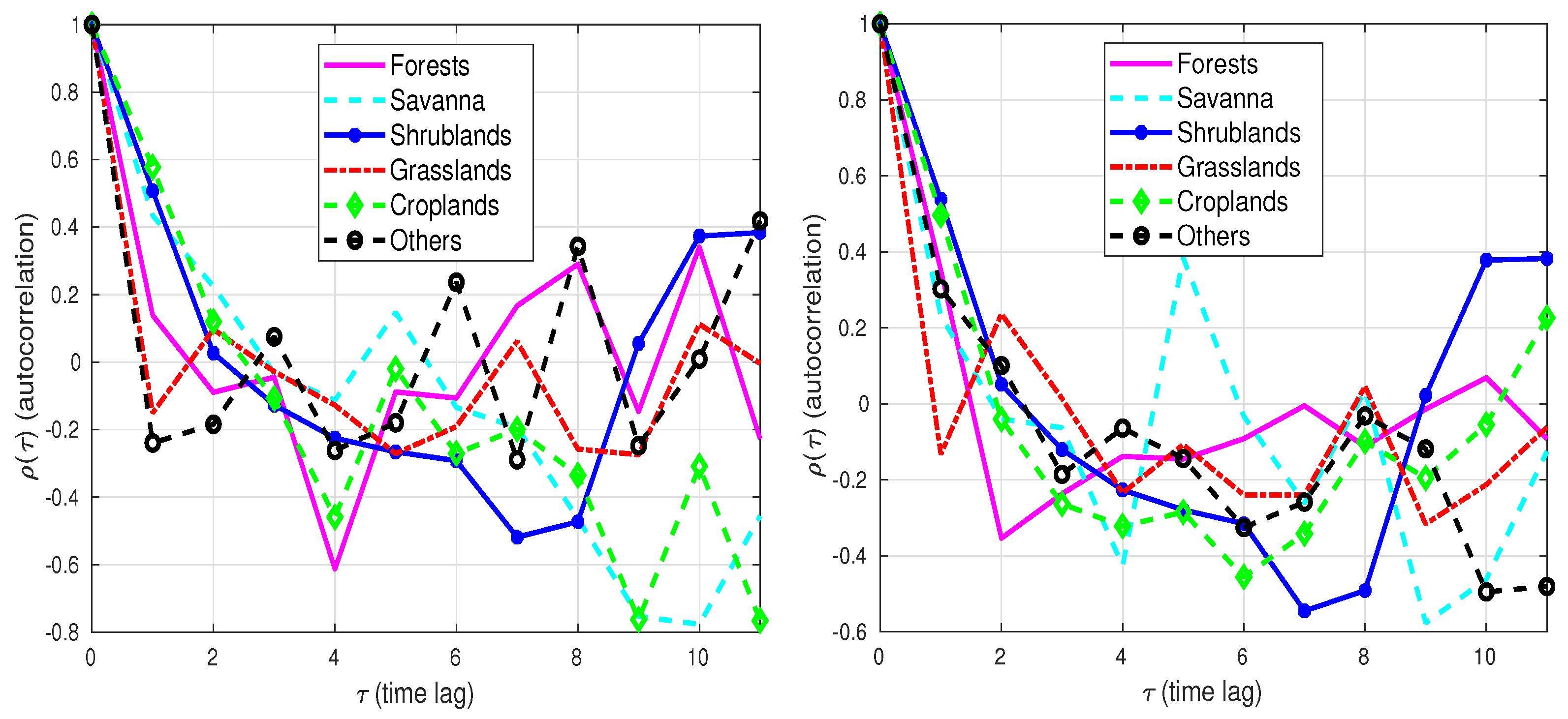
Savannas, grasslands, and croplands yielded linear gradient trends of −0.0048, −0.0007, and −0.0022 for the proportion of the burnt area that were all significant at 5% level. These trends correspond to decreases in the burnt area of 17,500, 1400, and 6300 km per annum for savannas, grasslands, and croplands, respectively. The forests showed an increasing linear gradient trend of 0.0002, with a p-value of 0.0104. Graphs of the power spectrum and autocorrelation for vegetation classes in northern sub-Saharan Africa are shown in Figure 8 and Figure 9, respectively. The period for the forests was 5 years via the autocorrelation function, 4 years via the power spectrum, and 4.73 years via nonlinear regression. Savanna fires showed a period of 5 years via both the autocorrelation function and nonlinear regression. Similarly, shrublands showed return times of around 5 years via both the autocorrelation function and nonlinear regression. On the basis of the autocorrelation function, grasslands yielded periods of 2.5 and 8 years, and nonlinear regression gave a period of 6.5 years. Croplands gave 4 years via both the autocorrelation function and power spectrum. Nonlinear regression gave a period of 5.9 for croplands.
3.4. Southern Hemisphere Africa: Vegetation-Specific
In southern-hemisphere Africa, significant nonzero linear trends were shown only for savanna and grasslands at values of −0.0015 and −0.0011, respectively. These trend values correspond to decreases in the burnt area of approximately 9200 and 700 km per annum for savannas and grasslands, respectively. Shrublands, forests, and other vegetation classes gave nonsignificant/nonzero trends. For the assessment of underlying oscillations, relevant graphs are shown in Figure 8 and Figure 9. Savannas yielded a period of 5 years via the autocorrelation function. The nonlinear fit and power spectrum gave wildly different periods of 7.17 and 2.4 years, respectively. Forests yielded wildly different periods of 3, 5, 8, and 10 via the autocorrelation function. The nonlinear regression via least squares gave a period of 5.13 years, while the power spectrum gave a period of 3 years. For such a short dataset, we consider the longer periods less justifiable and took them to be numerical artefacts.
4. Discussion
In this paper, we considered the proportion of the burnt area in sub-Saharan Africa over two decades spanning from 2001 to 2020. At the continental scale, the observed significant declines in the proportions of the total burnt area were consistent with the recent results in [47], whose computations were based on the total burnt area during the period from 1998 to 2015. Assessing global trends, the authors found a blend of increasing trends in some regions and decreasing trends in others, with areas with declining trends outnumbering those with increasing trends. For tropical savannas and grasslands, they found strong contrasting trends in northern sub-Saharan Africa and southern-hemisphere Africa. Declining trends were found in the north and increasing trends in the south. In our analysis, in addition to considering all sub-Saharan Africa, we split it into two regions: north and south of the equator.
Over the whole of sub-Saharan Africa, we found a significant declining trend of the proportion of the burnt area, with all vegetation types pooled together. Similar results were found for pooled vegetation types north and south of the equator. Turning to specific vegetation types over all sub-Saharan Africa, we found savannas, grasslands, and croplands to have significantly declining trends over the two decades, while forests showed a significant increasing trend. The negative trends shown by croplands might be expected if farming is reduced in response to a reduction in rainfall or if other management techniques are adopted. Some small-scale farming may exist within the primary areas of fire occurrence, which farming might be undetectable using the current MODIS spatial resolution (500 m). Moreover, more than 95% of land in savannas is used as rangeland, with cropland being less than 5%. In northern sub-Saharan Africa, savannas, grasslands, and croplands showed significantly declining trends, while forests yielded no significant trend. In southern-hemisphere Africa, only savannas and grasslands yielded significantly declining trends, while shrublands and forests gave no significant trends. These results indicate that the main drivers of the declining trend at the continental scale are savannas and grasslands. Results for central Africa were presented in [48], finding declining trends for grasslands and savannas. The results here were at the continental scale, including north and south of the equator.
The aforementioned trends were observed within overriding oscillations. The periods of the oscillations were found using alternative approaches, all of which yielded similar values. The period of oscillation was between 4 and 6 years. This agrees with the theoretical values found in [49], whose nonlinear, dynamic model yielded oscillations of a period of around 4 years. Empirical results based on satellite data for California found cyclic patterns of a period from 5 to 7 years [42], of which the results are comparable to those of this paper, albeit for a different geographical region. The observed cycles are for aggregated information, are much more pronounced at the continental scale, and are less pronounced for specific vegetation classes and at subcontinental scales. However, the per-tree mean fire return interval can be as high as 17 years [50], while savannas and grasslands fire return intervals can be far less. For instance, the authors in [51] found savanna return intervals at Kruger National Park in South Africa between 5.6 and 7.3 years. These values are consistent with cycle periods in this paper, and affirm that the trends and overriding cycles observed here are largely driven by the savannas.
Understanding fire trends and their cyclic nature is an important step towards fire management. It is a necessary step towards developing fire models capable of predicting fire outbreaks at relevant spatial scales. In order to build such predictive models, one can explore and exploit teleconnections. Teleconnections were found between fires in different parts of Earth and the El Nino-Southern Oscillations (ENSO) [50,52]. While ENSO is used to predict terrestrial precipitation, the relationship between fires and precipitation can be complex. In particular, fires can increase or decline due to a decrease in precipitation [52].
5. Conclusions
Fires over sub-Saharan Africa show a significantly decreasing trend in an oscillatory fashion. The most dominant period (or recurrence time) of the oscillations is approximately 5 years; it is most pronounced at the aggregated scale, and less pronounced for individual vegetation types. The decreasing oscillatory trend appears to be collectively driven by savannas, grasslands, and croplands, and the found period is consistent with the fire return intervals for these specific vegetation types. This pattern of decreasing fires can be viewed to be in accordance with climatic projections that expect precipitation to decline. Less rainfall is correlated with a decrease in biomass, thus accounting for the decline in the proportion of the burnt area. Furthermore, declining precipitation may be linked to a reduction in lightning strikes, which are a contributor to some of the rangeland fires.
Author Contributions
Conceptualization, R.L.M. and K.D.; methodology, R.L.M. and K.D.; software, R.L.M. and K.D.; validation, R.L.M.; formal analysis, R.L.M.; resources, K.D.; writing—original draft preparation, R.L.M.; writing—review and editing, R.L.M. and K.D. All authors have read and agreed to the published version of the manuscript.
Funding
This research received no external funding.
Institutional Review Board Statement
Not applicable.
Informed Consent Statement
No humans were involved in the study.
Data Availability Statement
The used data were acquired from NASA’s Earth Observing System Data and Information System (EOSDIS, https://search.earthdata.nasa.gov/search).
Acknowledgments
The authors would like to thank three anonymous reviewers for their comments that helped in improving this manuscript.
Conflicts of Interest
The authors declare no conflict of interest. No funders had a role in the design of the study; in the collection, analyses, or interpretation of data; in the writing of the manuscript; or in the decision to publish the results.
References
- Glasspool, I.; Edwards, D.; Axe, L. Charcoal in the Silurian as evidence for the earliest wildfire. Geology 2004, 32, 381–383. [Google Scholar] [CrossRef]
- Hao, W.; Liu, M.H. Spatial and temporal distribution of tropical biomass burning. Glob. Biogeochem. Cycles 1994, 8, 495–503. [Google Scholar] [CrossRef]
- Tansey, K.; Grégoire, J.M.; Binaghi, E.; Boschetti, L.; Ershov, D.; Flasse, S.; Fraser, R.; Graetz, D.; Maggi, M.; Peduzzi, P.; et al. A Global Inventory of Burned Areas at 1 Km Resolution for the Year 2000 Derived from Spot Vegetation Data. Clim. Chang. 2004, 67, 345–377. [Google Scholar] [CrossRef]
- Lipsett-Moore, G.J.; Wolff, N.H.; Game, E.T. Emissions mitigation opportunities for savanna countries from early dry season fire management. Nat. Commun. 2018, 9, 2247. [Google Scholar] [CrossRef] [PubMed] [Green Version]
- Grunow, J.O.; Groenveld, H.T.; Du Troit, S.H.C. Above-Ground Dry Matter Dynamics of the Grass Layer of a South African Tree Savanna. J. Ecol. 1980, 68, 877–889. [Google Scholar] [CrossRef]
- Ramankutty, N.; Foley, J.A. Estimating Historical Changes in Global Land Cover: Croplands from 1700 to 1992. Glob. Biogeochem. Cycles 1999, 13, 997–1027. [Google Scholar] [CrossRef]
- Smit, G. An approach to tree thinning to structure southern African savannas for long-term restoration from bush encroachment. J. Environ. Manag. 2004, 71, 179–191. [Google Scholar] [CrossRef]
- Kgope, B.S.; Bond, W.J.; Mingley, G.F. Growth Responses of African Savanna Trees Implicate Atmospheric [CO2] as a Driver of Past and Current Changes in Savanna Tree Cover. Austral Ecol. 2010, 35, 451–463. [Google Scholar] [CrossRef]
- Shackleton, C.M.; Scholes, R.J. Above Ground Woody Community Attributes, Biomass and Carbon Stocks along a Rainfall Gradient in the Savannas of the Central Lowveld, South Africa. S. Afr. J. Bot. 2011, 77, 184–192. [Google Scholar] [CrossRef] [Green Version]
- Fuller, G.D. The Geobotany and Soils of Africa. Ecology 1924, 5, 205–207. [Google Scholar] [CrossRef]
- Scholes, R.J.; Archer, S.R. Tree-Grass interactions in savannas. Annu. Rev. Ecol. Syst. 1997, 28, 517–544. [Google Scholar] [CrossRef]
- Grace, J.; Jose, J.S.; Meir, P.; Miranda, H.S.; Montes, R.A. Productivity and carbon fluxes of tropical savannas. J. Biogeogr. 2006, 33, 387–400. [Google Scholar] [CrossRef]
- Ingvar, B. Distribution and Vegetation Dynamics of Humid Savannas in Africa and Asia. J. Veg. Sci. 1992, 3, 345–356. [Google Scholar]
- Chen, X.; Hutley, L.B.; Eamus, D. Carbon Balance of a Tropical Savanna of Northern Australia. Oecologia 2003, 137, 405–416. [Google Scholar] [CrossRef] [PubMed]
- Blydenstein, J. Tropical Savanna Vegetation of Llanos of Colombia. Ecology 1967, 48, 1–15. [Google Scholar] [CrossRef]
- Goodland, R.; Pollard, R. The Brazilian Cerrado Vegetation: A Fertility Gradient. J. Ecol. 1973, 61, 219–224. [Google Scholar] [CrossRef]
- Medina, E.; Silva, J.F. Savannas of Northern South America: A Steady State Regulated by Water-Fire Interactions on a Background of Low Nutrient Availability. J. Biogeogr. 1990, 17, 403–413. [Google Scholar] [CrossRef]
- Romero-Ruiz, M.; Etter, A.; Sarmiento, A.; Tansey, K. Spatial and temporal variability of fires in relation to ecosystems, land tenure and rainfall in savannas of northern South America. Glob. Chang. Biol. 2010, 16, 2013–2023. [Google Scholar] [CrossRef]
- Hartmann, D.; Klein Tank, A.M.G.; Rusticucci, M.; Alexander, L.V.; Bronnimann, S.; Charabi, Y.; Dentener, F.J.; Dlugokencky, E.J.; Easterling, D.R.; Kaplan, A.; et al. Observations: Atmosphere and Surface. In Climate Change 2013: The Physical Science Basis. Contribution of Working Group I to the Fifth Assessment Report of the Intergovernmental Panel on Climate Change; Stocker, T.F., Qin, D., Plattner, G.K., Tignor, M., Allen, S.K., Boschung, J., Nauels, A., Xia, Y., Bex, V., Midgley, P.M., Eds.; Cambridge University Press: Cambridge, UK; New York, NY, USA, 2013. [Google Scholar]
- Knapp, A.; Beier, C.; Briske, D.; Classen, A.; Luo, Y.; Reichstein, M.; Smith, M.; Smith, S.; Bell, J.; Fay, P.; et al. Consequences of More Extreme Precipitation Regimes for Terrestrial Ecosystems. BioScience 2008, 58, 811–821. [Google Scholar] [CrossRef]
- Shongwe, M.; van Oldenborgh, G.; van den Hurk, B.; de Boer, B.; Coelho, C.; van Aalst, M. Projected Changes in Mean and Extreme Precipitation in Africa under Global Warming. Part I: Southern Africa. J. Clim. 2009, 22, 3819–3837. [Google Scholar] [CrossRef]
- Cao, M.; Zang, Q.; Shuggart, H.H. Dynamic Response of African ecosystem carbon cycling to climate change. Clim. Res. 2001, 17, 183–193. [Google Scholar] [CrossRef]
- Dintwe, K.; Okin, G.S.; D’Odorico, P.; Hrast, T.; Mladenov, N.; Handorean, A.; Battachan, A.; Caylor, K.K. Soil organic C and total N pools in the Kalahari: Potential impacts on C sequenstration in Savanna. Plant Soil 2014, 396, 27–44. [Google Scholar] [CrossRef]
- Hoffmann, W.; Schroeder, W.; Jackson, R. Positive feedbacks of fire, climate, and vegetation and the conversion of tropical savanna. Geophys. Res. Lett. 2002, 29, 9/1–9/4. [Google Scholar] [CrossRef] [Green Version]
- Liu, Y.; Stanturf, J.; Goodrick, S. Trends in global wildfire potential in a changing climate. For. Ecol. Manag. 2010, 259. [Google Scholar] [CrossRef]
- Shongwe, M.; van Oldenborgh, G.; van den Hurk, B.; van Aalst, M. Projected Changes in Mean and Extreme Precipitation in Africa under Global Warming. Part II: East Africa. J. Clim. 2011, 24, 3718–3733. [Google Scholar] [CrossRef] [Green Version]
- Biasutti, M. Rainfall trends in the African Sahel: Characteristics, processes and causes. WIREs Clim. Chang. 2019, 10, e591. [Google Scholar] [CrossRef] [Green Version]
- Tyson, P.D.; Crimp, S.J. The Climate of the Kalahari Transect. Trans. R. Soc. S. Afr. 1998, 53, 93–112. [Google Scholar] [CrossRef]
- Caylor, K.K.; Shugart, H.H.; Dowty, P.R.; Smith, T.M. Tree Spacing along the Kalahari Transect in Southern Africa. J. Arid Environ. 2003, 54, 281–296. [Google Scholar] [CrossRef] [Green Version]
- Cahoon, D.R.J.; Stocks, B.J.; Levine, J.S.; Cofer, W.R., III; O’Neill, K.P. Seasonal Distribution of African Savanna Fires. Nature 1992, 359, 812–815. [Google Scholar] [CrossRef]
- Cooke, W.F.; Koffi, B.; Gregoire, J.M. Seasonality of vegetation fires in Africa from remote sensing data and application to a global chemistry model. J. Geophys. Res. Atmos. 1992, 101, 21051–21065. [Google Scholar] [CrossRef]
- D’Odorico, P.; Caylof, K.; Okin, G.S.; Scanlon, T.M. On soil moisture-vegetation feedbacks and their possible effects on the dynamics of dryland ecosystems. J. Geophys. Res. Biogeosci. 2004, 112, G04010. [Google Scholar] [CrossRef] [Green Version]
- Flanagan, L.B.; Wever, L.A.; Carlson, P.J. Seasonal and interannual variation in carbon dioxide exchange and carbon balance in a northern temperate grassland. Glob. Chang. Biol. 2002, 8, 599–615. [Google Scholar] [CrossRef]
- Scholes, R.J. Greenhouse gas emissions from vegetation fires in southern Africa: Environ. Monit. Assess. 1995, 38/2–3 (169–179). Summ. in Engl. Environ. Pollut. 1996, 94, 169–179. [Google Scholar] [CrossRef]
- van der Werf, G.; Randerson, J.; Giglio, L.; Collatz, G.; Kasibhatla, P.; Arellano, A., Jr. Interannual variability in global biomass burning emissions from 1997 to 2004. Atmos. Chem. Phys. 2006, 6, 3423–3441. [Google Scholar] [CrossRef] [Green Version]
- Archer, S.; Boutton, T.W.; Hibbard, K.A. Trees in Grasslands: Biogeochemical Consequences of Woody Plant Expansion. In Global Biogeochemical Cycles in the Climate System; Schulze, E.D., Heimann, M., Harrison, S., Holland, E., Loyd, J., Prentice, I.C., Schimel, D., Eds.; Academic Press: San Diego, CA, USA, 2001; pp. 115–137. [Google Scholar]
- Dintwe, K.; Okin, G.S.; Hue, Y. Fire-induced albedo change and surface radiative forcing in sub-Saharan Africa savanna ecosystems: Implications for the energy balance. J. Geophys. Res. Atmos. 2017, 122, 6186–6201. [Google Scholar] [CrossRef] [Green Version]
- Roy, D.P.; Boschetti, L.; Justice, C.O.; Ju, J. The collection 5 MODIS burned area product—Global evaluation by comparison with the MODIS active fire product. Remote Sens. Eviron. 2008, 112, 3690–3707. [Google Scholar] [CrossRef]
- Nelder, J.; Wedderburn, R. Generalised Linear Models. J. R. Stat. Soc. Ser. A 1972, 135, 370–384. [Google Scholar] [CrossRef]
- Barth, J.R.; Bennett, J.T. Cyclic behavior, seasonality and trends in economic time series. Neb. J. Econ. Bus. 1974, 13, 48–69. [Google Scholar]
- Roger, J.H. A significance test for cyclic trends in incidence data. Biometrika 1977, 64, 152–155. [Google Scholar] [CrossRef]
- Son, R.; Wang, S.-Y.S.; Kim, S.H.; Kim, H.; Jeong, J.H. Recurrent pattern of extreme fire weather in California. Environ. Res. Lett. 2021, 16, 094031. [Google Scholar] [CrossRef]
- Proakis, J.G.; Manolakis, D.G. Digital Signal Processing: Principles, Algorithms and Applications, 3rd ed.; Prentice-Hall International: Hoboken, NJ, USA, 1996. [Google Scholar]
- Dirac, P. Principles of Quantum Mechanics, 1st ed.; Oxford University Press: Oxford, UK, 1930. [Google Scholar]
- Podschwit, H.; Guttorp, P.; Larkin, H.; Steel, E.A. Estimating wildfire growth from noisy and incomplete incident data using a state space model. Environ. Ecol. Stat. 2018, 25, 325–340. [Google Scholar] [CrossRef] [Green Version]
- Thayjes, S. Wildfire Spread Prediction and Assimilation for FARSITE Using Ensemble Kalman Filtering. Ph.D. Thesis, University of California, San Diego, CA, USA, 2016. [Google Scholar]
- Andela, N.; Morton, D.C.; Giglio, L.; Chen, Y.; van der Werf, G.R.; Kasibhatla, P.S.; Defrie, R.S.; Collatz, G.J.; Hantso, S.; Kloster, S.; et al. A human-driven decline in global burned area. Science 2017, 356, 1356–1362. [Google Scholar] [CrossRef] [PubMed] [Green Version]
- Jiang, Y.; Zhou, L.; Raghavenda, A. Observed changes in patterns and possible drivers over Central Africa. Environ. Res. Lett. 2020, 15, 0940b8. [Google Scholar] [CrossRef]
- Farkondehmaal, F.; Ghaffarzadegan, N. A cyclical wildfire pattern as the outcome of a coupled human natural system. Sci. Rep. 2022, 12, 5280. [Google Scholar] [CrossRef]
- Yocom, L.L.; Fule, P.Z.; Brown, P.M.; Cerano, J.; Villanueza-Diaz, J.; Falk, D.A.; Cornejo-Oviedo, E. El Nino-southern oscillation effect on fire regime in northeastern Mexico has changed over time. Ecology 2010, 91, 1660–1671. [Google Scholar] [CrossRef] [PubMed] [Green Version]
- Van Wilgen, B.W.; Govender, N.; Biggs, H.C.; Ntsala, D.; Funda, X.N. Response of savanna fire regimes to changing fire-management policies in a large African national park. Conserv. Biol. 2004, 18, 1533–1540. [Google Scholar] [CrossRef]
- Le, T.; Kim, S.H.; Bae, D.H. Decreasing causal impacts of El Nino Southern Oscillation on future fire activities. Sci. Total Environ. 2022, 826, 154031. [Google Scholar] [CrossRef]
Figure 1.
Map of the vegetation classes in Africa following International Geosphere–Biosphere Programme (IGBP) land cover classification. NSSA is northern sub-Saharan Africa, while SHA is southern-hemisphere Africa. The two regions, separated by the equator (represented by a back dotted line), together constitute sub-Saharan Africa (SSA). This map was adopted from [37].

Figure 2.
Graphs of two signals corrupted with noise of varying strength. The signal on the left has a single frequency, while the one on the right is a superposition of two signals of different frequencies and amplitudes. The colour bar on the right reflects the proportion of noise added to the signal, .
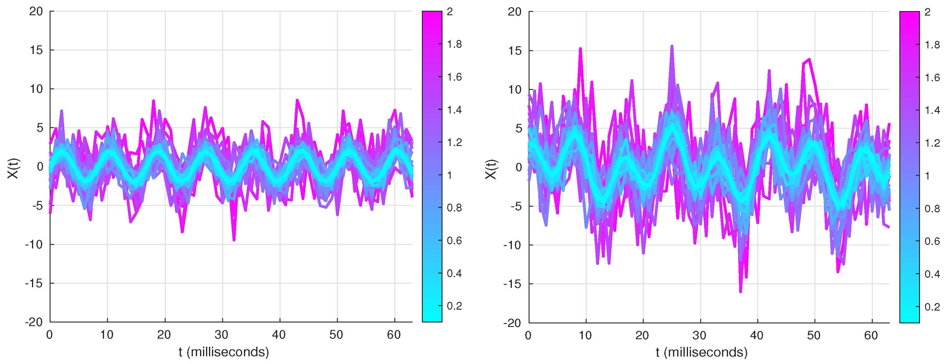
Figure 3.
Graphs to highlight the efficacy of a power spectrum and autocorrelation to detect underlying frequencies. The top graphs are power spectra, while bottom graphs are the autocorrelation function for the two signals in Figure 2. The colour bar on the right is the proportion of noise to signal, .

Figure 4.
Graphs of fire trends from 2001 to 2020 for the entirety of sub-Saharan Africa. Positive latitude values are northward while positive longitude values are eastward. The value of 0 latitude corresponds to the equator, and the value of 0 longitude corresponds to the prime meridian line.
Figure 4.
Graphs of fire trends from 2001 to 2020 for the entirety of sub-Saharan Africa. Positive latitude values are northward while positive longitude values are eastward. The value of 0 latitude corresponds to the equator, and the value of 0 longitude corresponds to the prime meridian line.
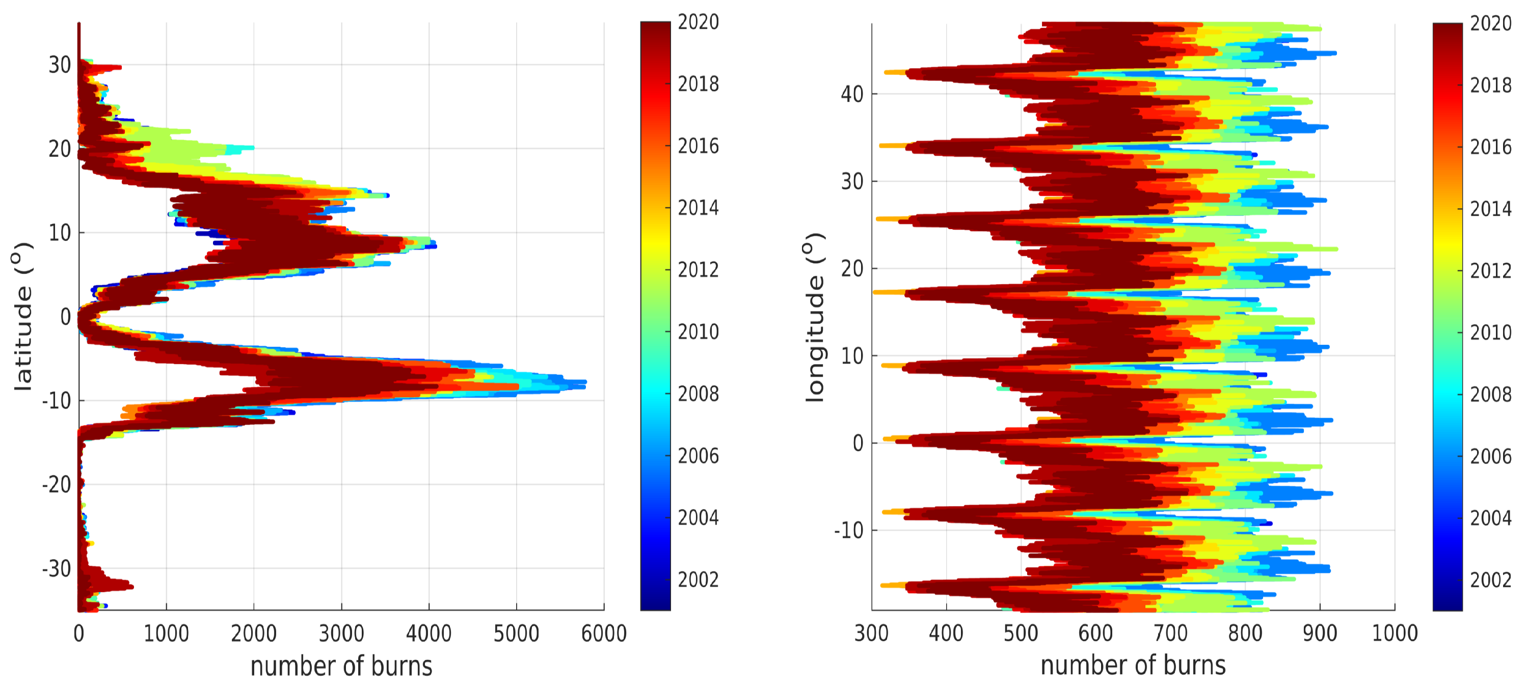
Figure 5.
Graphs showing the trends of aggregated fires over all sub-Saharan Africa, southern-hemisphere Africa, and northern sub-Saharan Africa. Plus signs are the actual observation points, dotted lines are the linear regression fits, and the solid line is the fitted oscillatory line using nonlinear least squares.

Figure 6.
Graphs of the power spectrum as a function of frequency and autocorrelation as a function of lag time applied to the time series of the proportion of the burnt area for aggregated vegetation types in sub-Saharan Africa.
Figure 6.
Graphs of the power spectrum as a function of frequency and autocorrelation as a function of lag time applied to the time series of the proportion of the burnt area for aggregated vegetation types in sub-Saharan Africa.

Figure 7.
Graphs of the power spectrum as a function of frequency and autocorrelation versus lag time applied to the time series of the proportion of the burnt area for different vegetation types over all sub-Saharan Africa.
Figure 7.
Graphs of the power spectrum as a function of frequency and autocorrelation versus lag time applied to the time series of the proportion of the burnt area for different vegetation types over all sub-Saharan Africa.
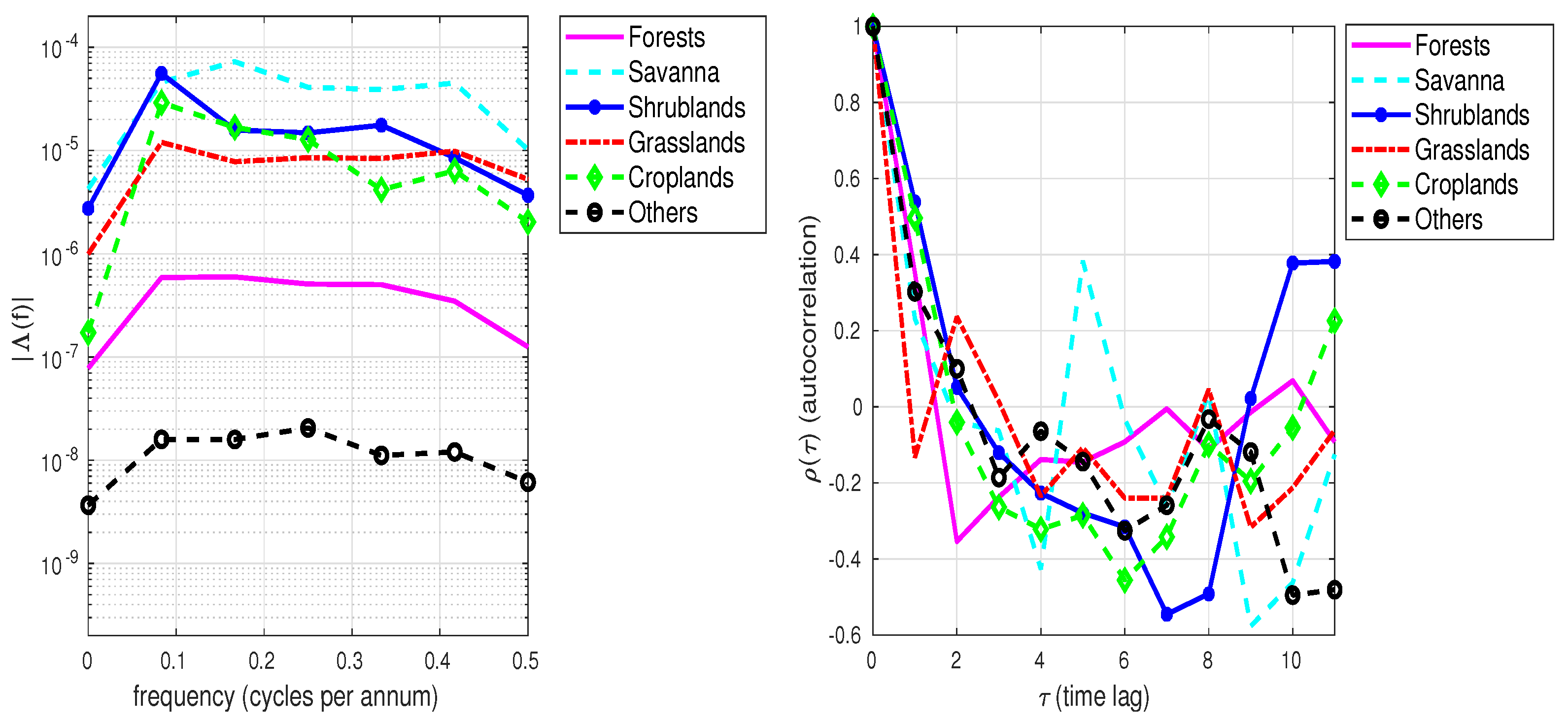
Figure 8.
Graphs of the power spectrum as a function of frequency applied to the time series of the proportion of the burnt area for different vegetation types in (left) southern-hemisphere Africa and (right) northern sub-Saharan Africa.
Figure 8.
Graphs of the power spectrum as a function of frequency applied to the time series of the proportion of the burnt area for different vegetation types in (left) southern-hemisphere Africa and (right) northern sub-Saharan Africa.
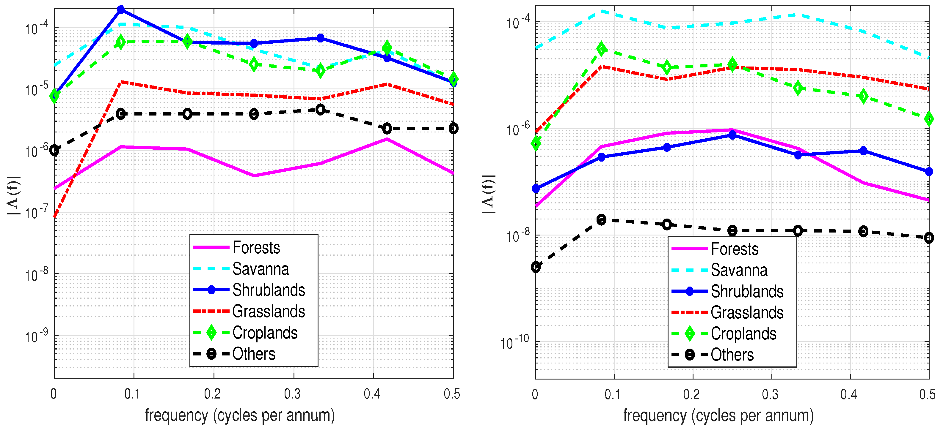
Figure 9.
Graphs of autocorrelation as a function of the time lag applied to the time series of the proportion of the burnt area for different vegetation types in (left) southern-hemisphere Africa and (right) northern sub-Saharan Africa.
Figure 9.
Graphs of autocorrelation as a function of the time lag applied to the time series of the proportion of the burnt area for different vegetation types in (left) southern-hemisphere Africa and (right) northern sub-Saharan Africa.
Disclaimer/Publisher’s Note: The statements, opinions and data contained in all publications are solely those of the individual author(s) and contributor(s) and not of MDPI and/or the editor(s). MDPI and/or the editor(s) disclaim responsibility for any injury to people or property resulting from any ideas, methods, instructions or products referred to in the content. |
© 2023 by the authors. Licensee MDPI, Basel, Switzerland. This article is an open access article distributed under the terms and conditions of the Creative Commons Attribution (CC BY) license (https://creativecommons.org/licenses/by/4.0/).
Share and Cite
MDPI and ACS Style
Machete, R.L.; Dintwe, K. Cyclic Trends of Wildfires over Sub-Saharan Africa. Fire 2023, 6, 71. https://doi.org/10.3390/fire6020071
AMA Style
Machete RL, Dintwe K. Cyclic Trends of Wildfires over Sub-Saharan Africa. Fire. 2023; 6(2):71. https://doi.org/10.3390/fire6020071
Chicago/Turabian StyleMachete, Reason L., and Kebonyethata Dintwe. 2023. "Cyclic Trends of Wildfires over Sub-Saharan Africa" Fire 6, no. 2: 71. https://doi.org/10.3390/fire6020071