
Benchmarking Studies Aimed at Clustering and Classification Tasks Using K-Means, Fuzzy C-Means and Evolutionary Neural Networks


Abstract
:1. Introduction
2. Materials and Methods
2.1. K-Means Algorithm
- The number of iterations exceeds a predefined maximum.
- When change in the cluster centroids is negligible.
- When there is no cluster membership change.
2.2. Fuzzy C-Means Algorithm
2.3. Feed Forward Neural Network with a Particle Swarm Optimization (PSO) Driven Weight Update Scheme
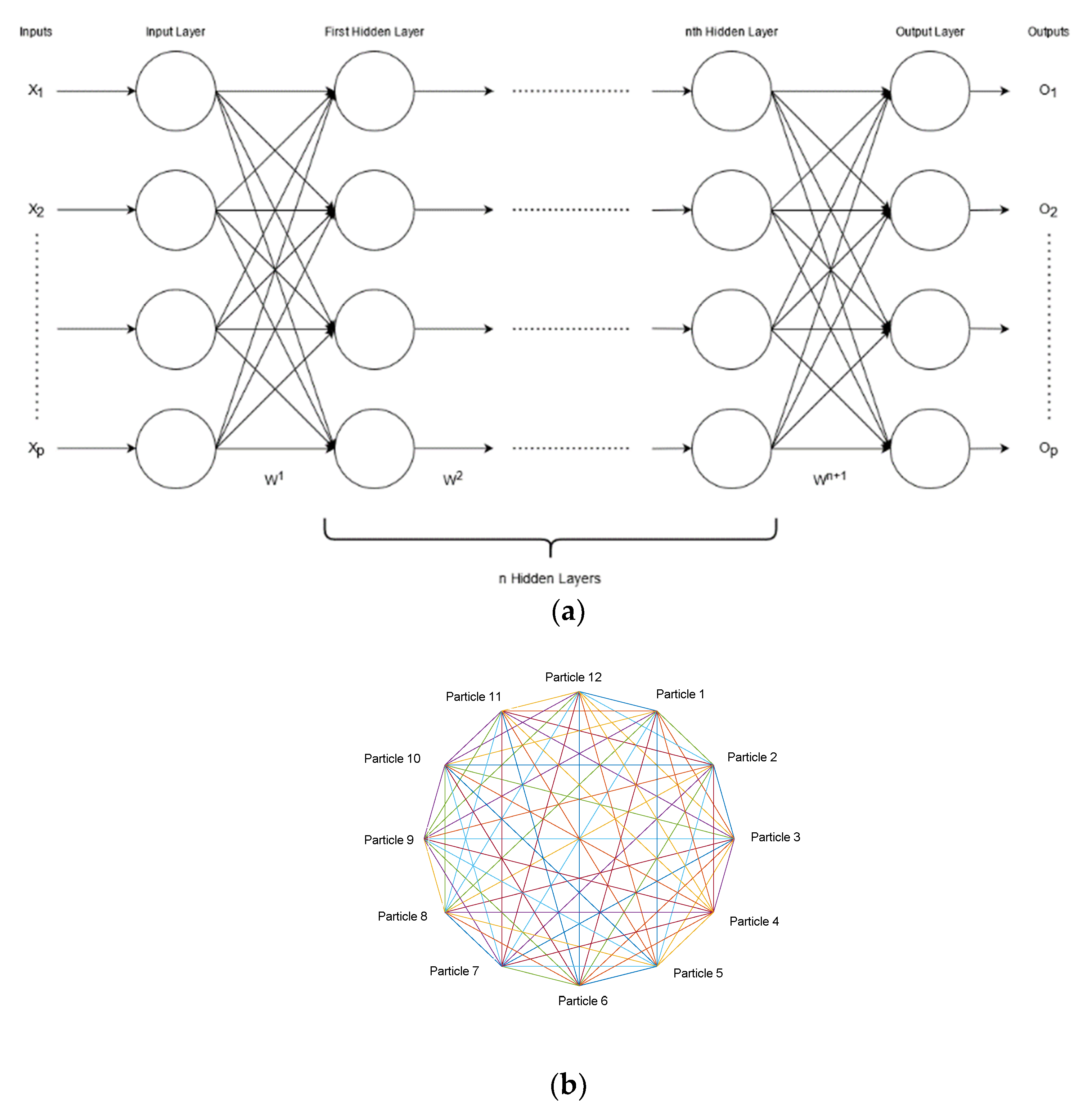
2.3.1. Feed-Forward Neural Network
2.3.2. Particle Swarm Optimization (PSO)
3. Experimental Setup
3.1. Parameter Settings for PSO
3.2. Data Sets
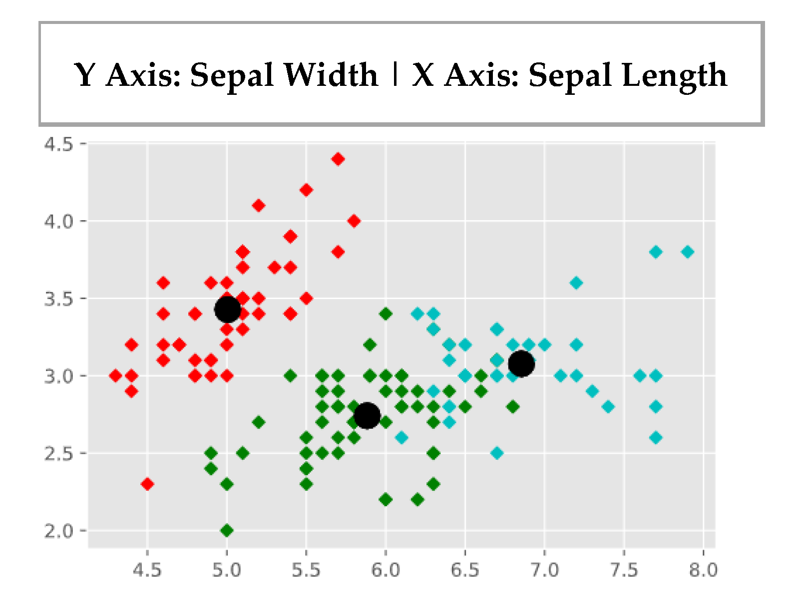
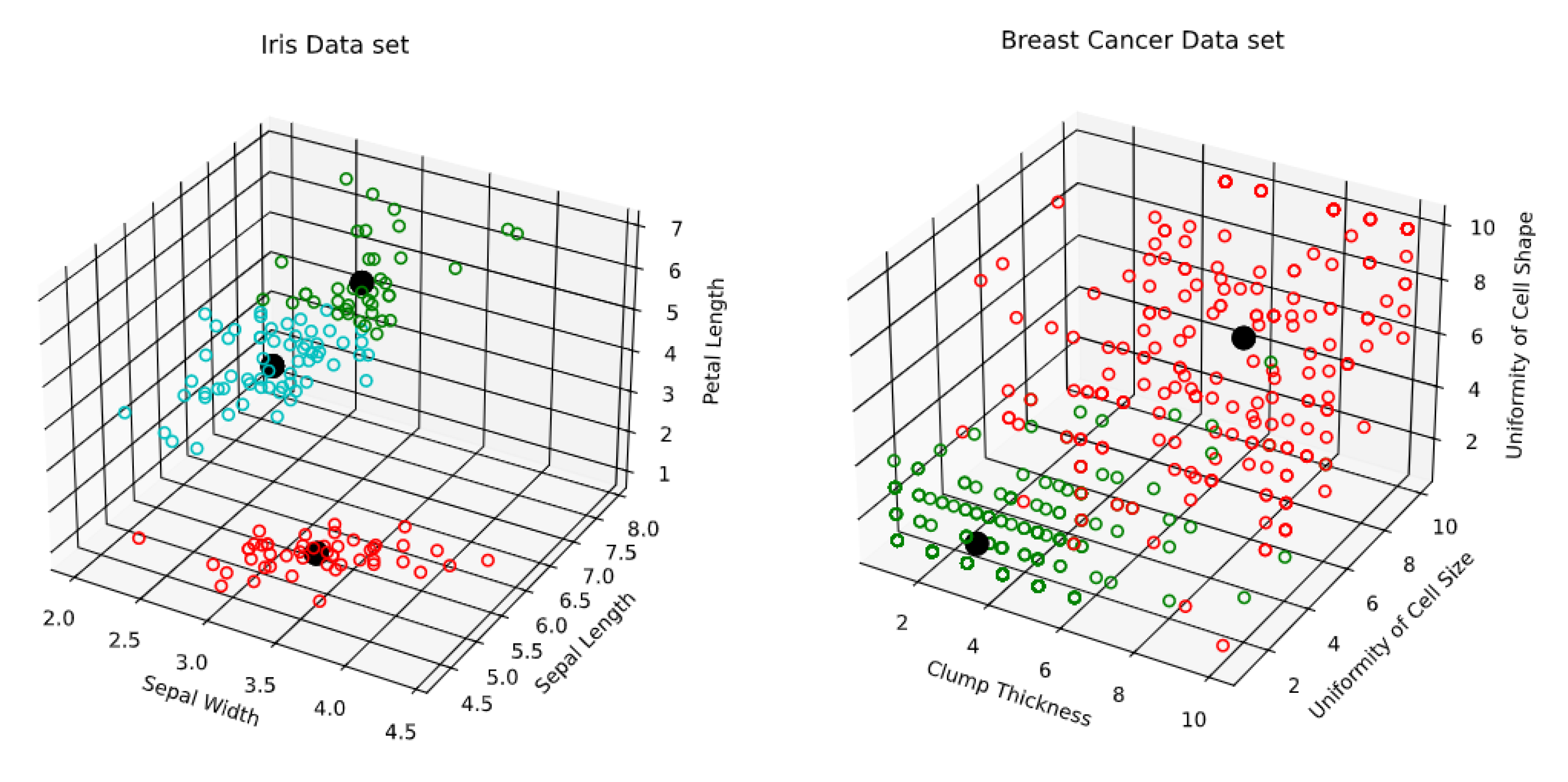
- 1.
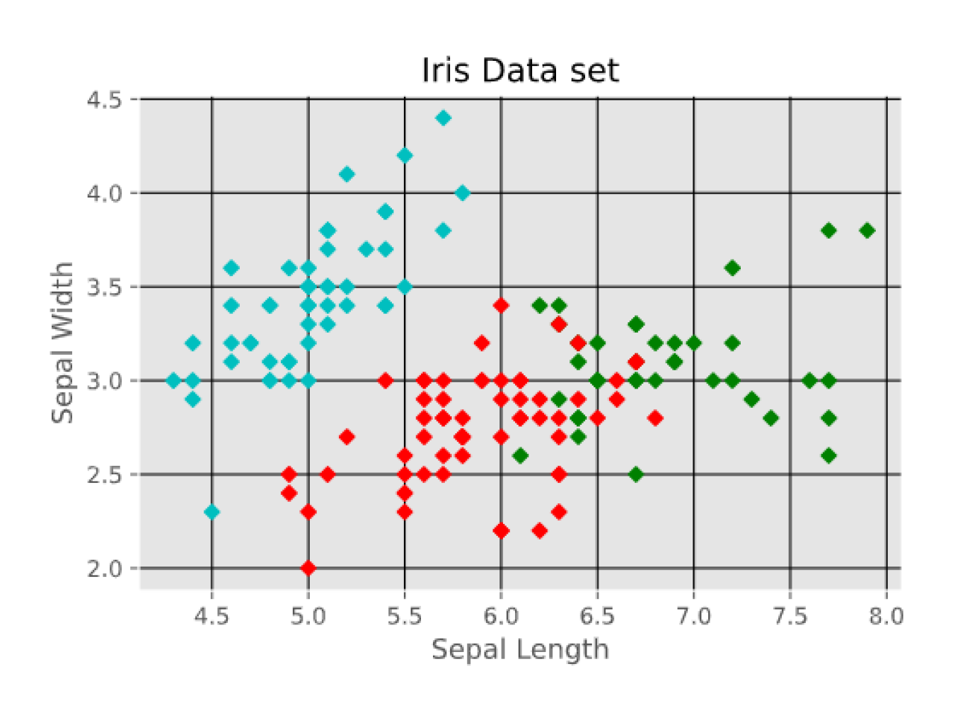
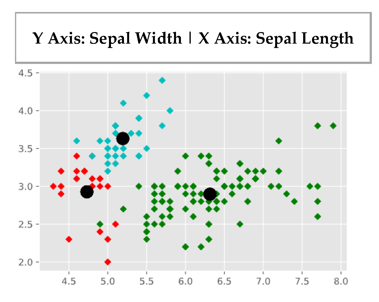
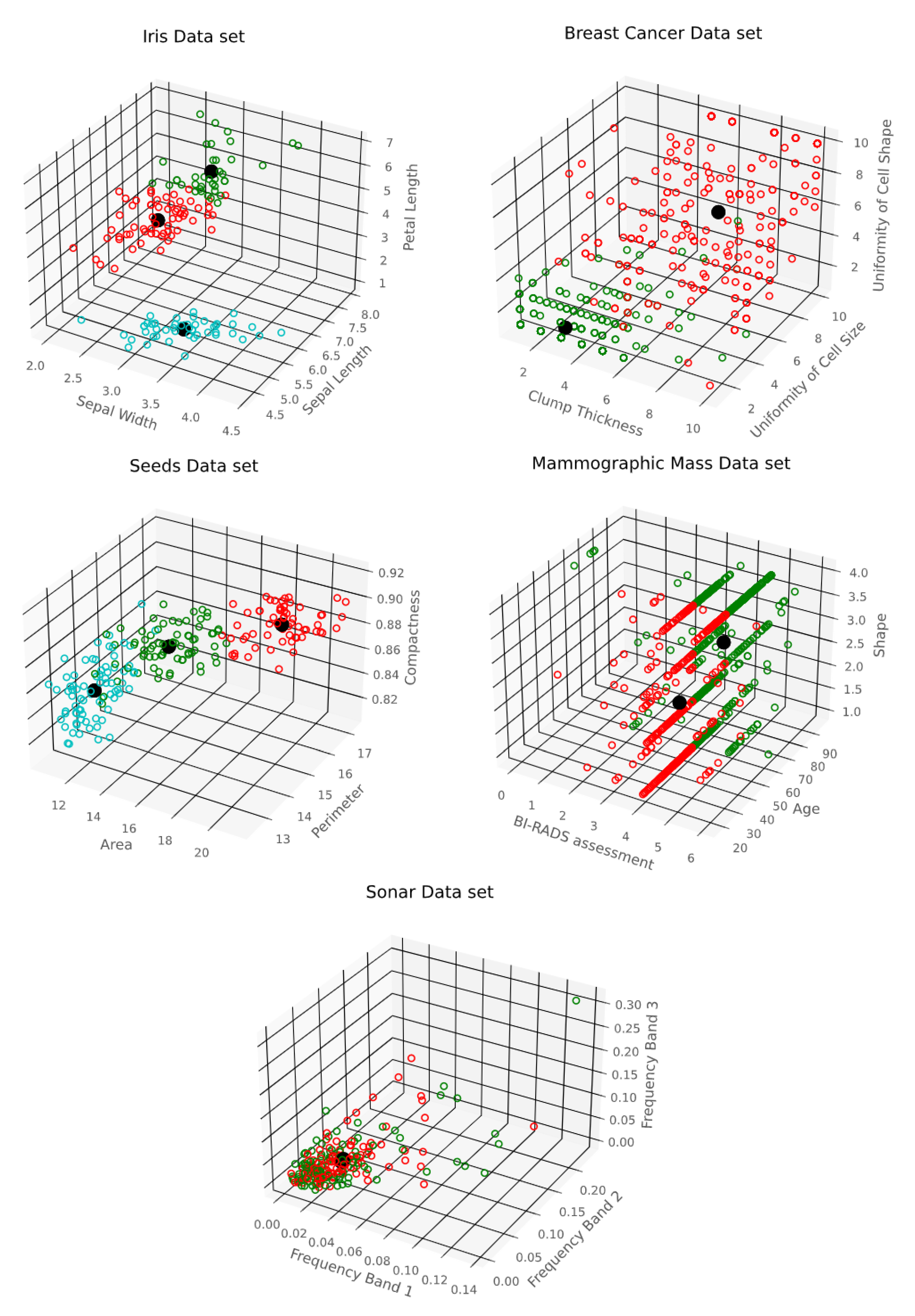
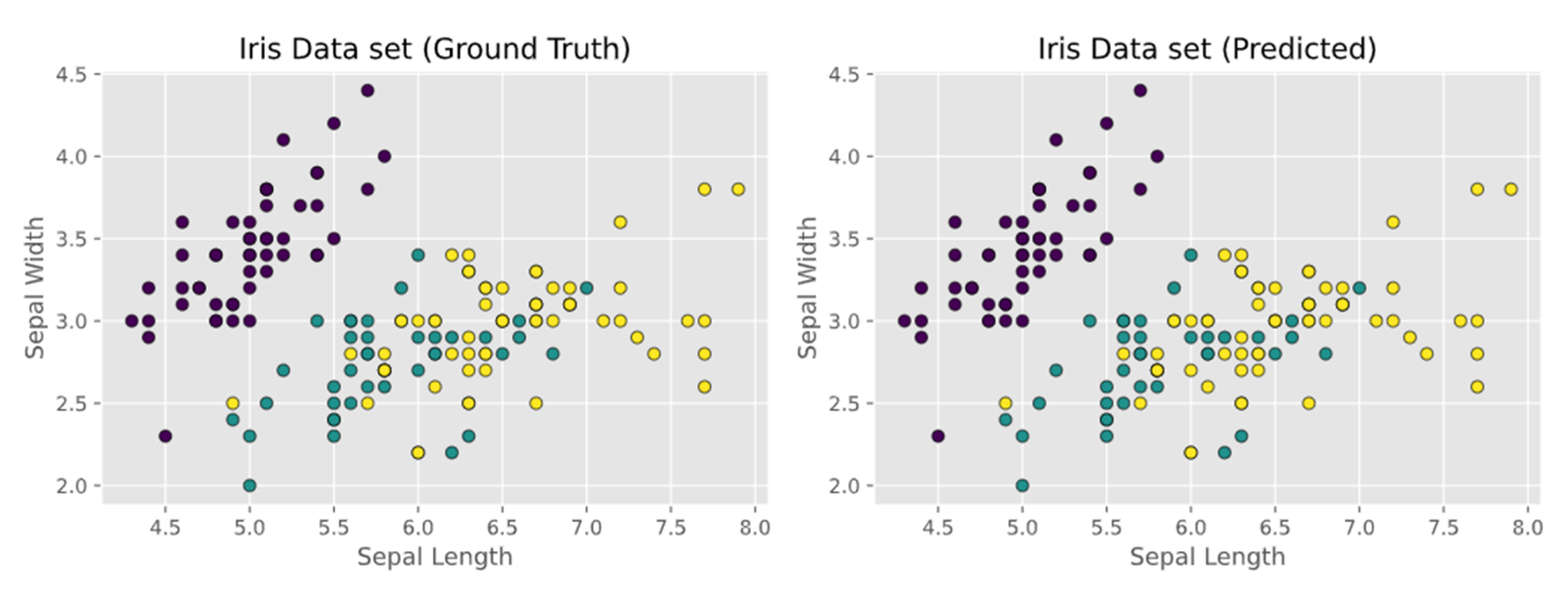
- R. A. Fisher’s Iris data set covering three species of Iris flowers (Setosa, Versicolor, and Virginica) containing a total of 150 instances with 4 attributes each. The attributes are as follows: sepal length, sepal width, petal length and petal width. The first two attributes i.e. Sepal Length and Sepal Width are shown in Figure 3.
- 2.
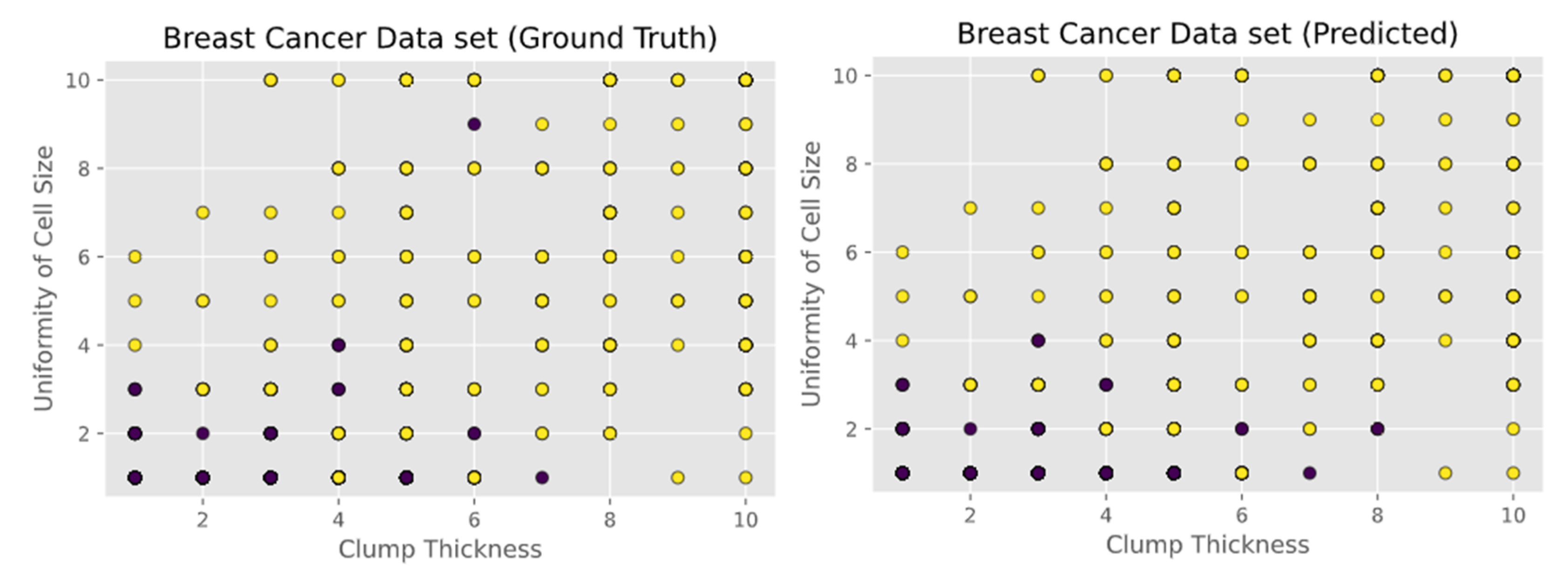
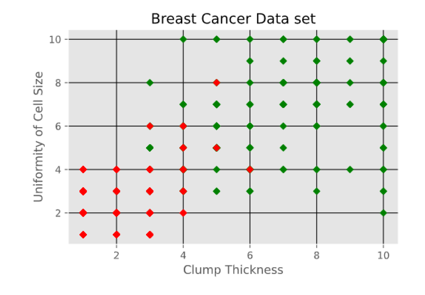
- Breast Cancer Wisconsin (Original) data set consisting of 699 instances and containing 10 attributes. Instances are classified into one of two categories, benign or malignant. The attributes are as follows: clump thickness, uniformity of cell size, uniformity of cell shape, marginal adhesion, single epithelial cell size, bare nuclei, bland chromatin, normal nucleoli, and mitoses. The first two attributes i.e. Clump Thickness and Uniformity of Cell Size are shown in Figure 4.
- 3.
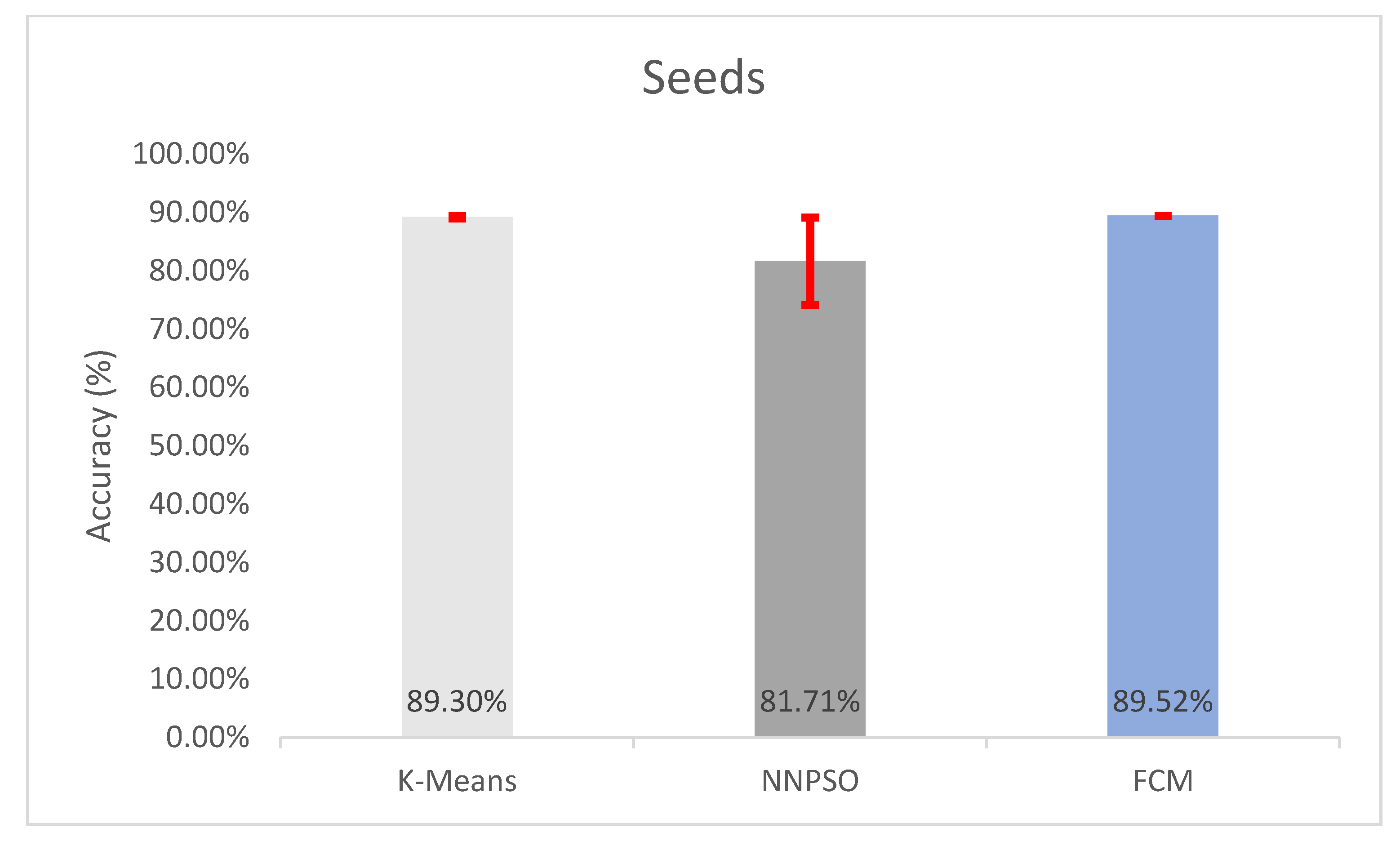
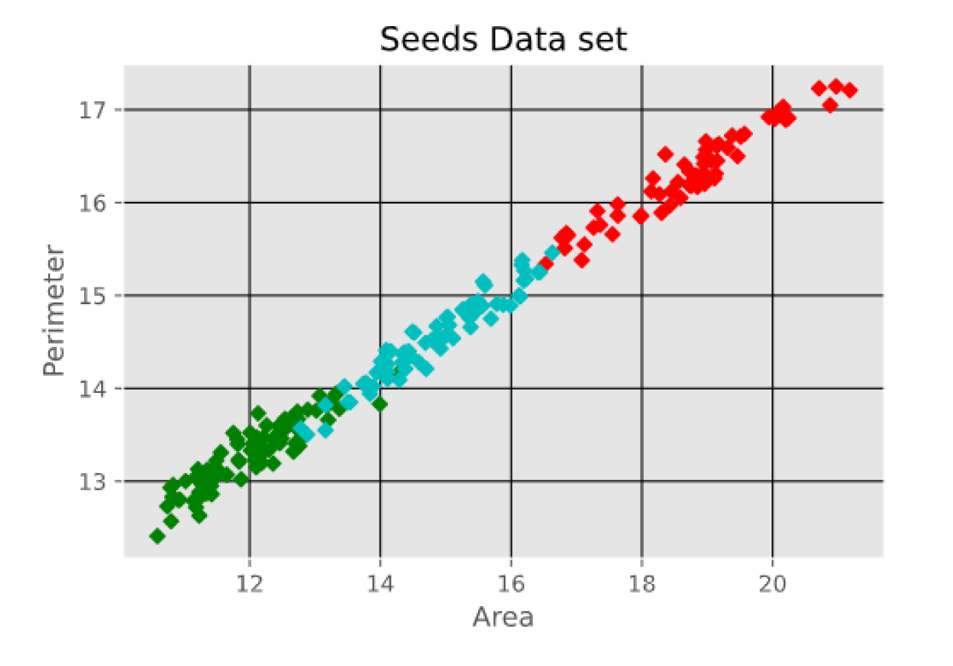
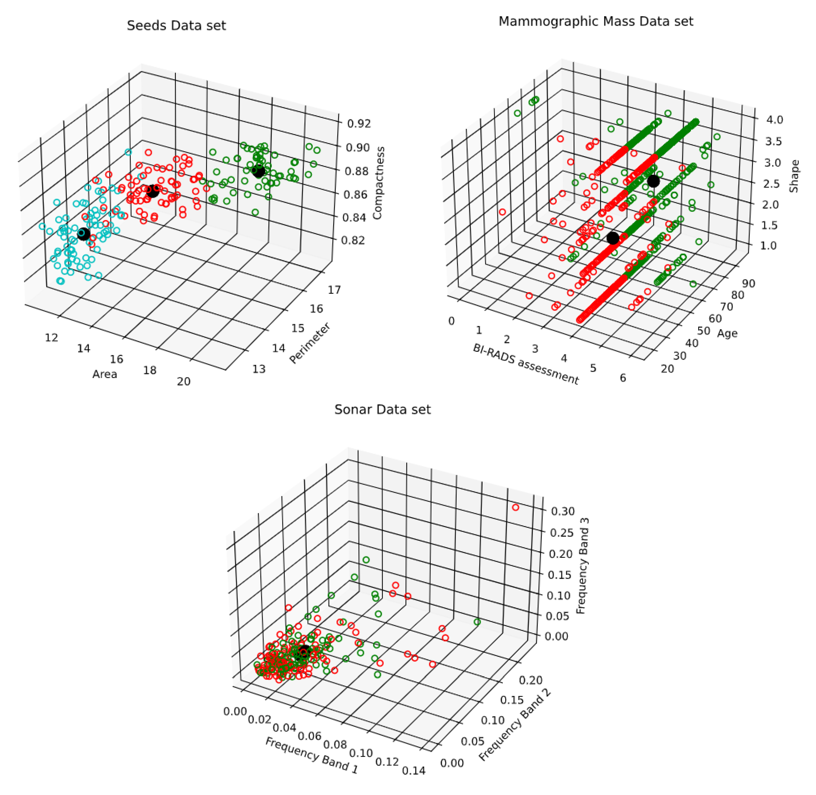
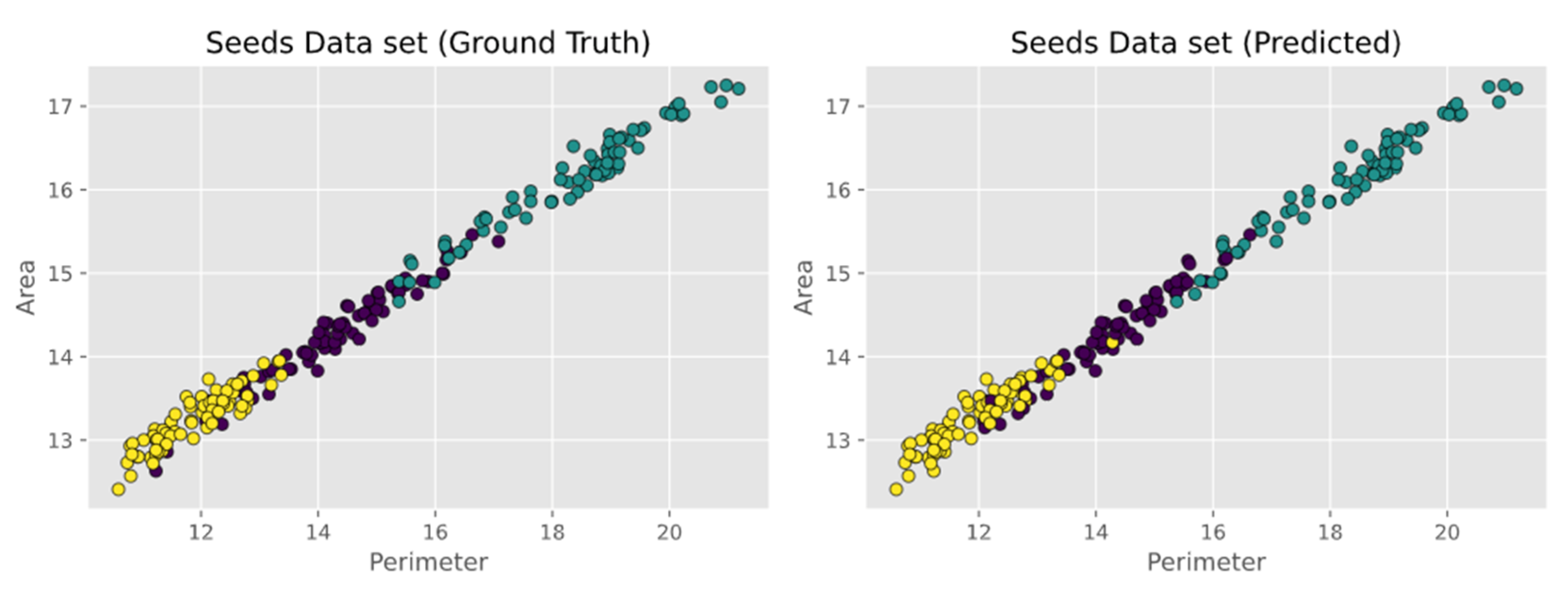
- Seeds data set, which is used to identify 3 different varieties of wheat: Kama, Rosa, and Canadian. The data set contains 210 instances with 7 attributes each. The attributes are as follows: area, perimeter, compactness, length of kernel, width of kernel, asymmetry coefficient, and length of kernel groove. The first two attributes i.e. Area and Perimeter are shown in Figure 5.
- 4.
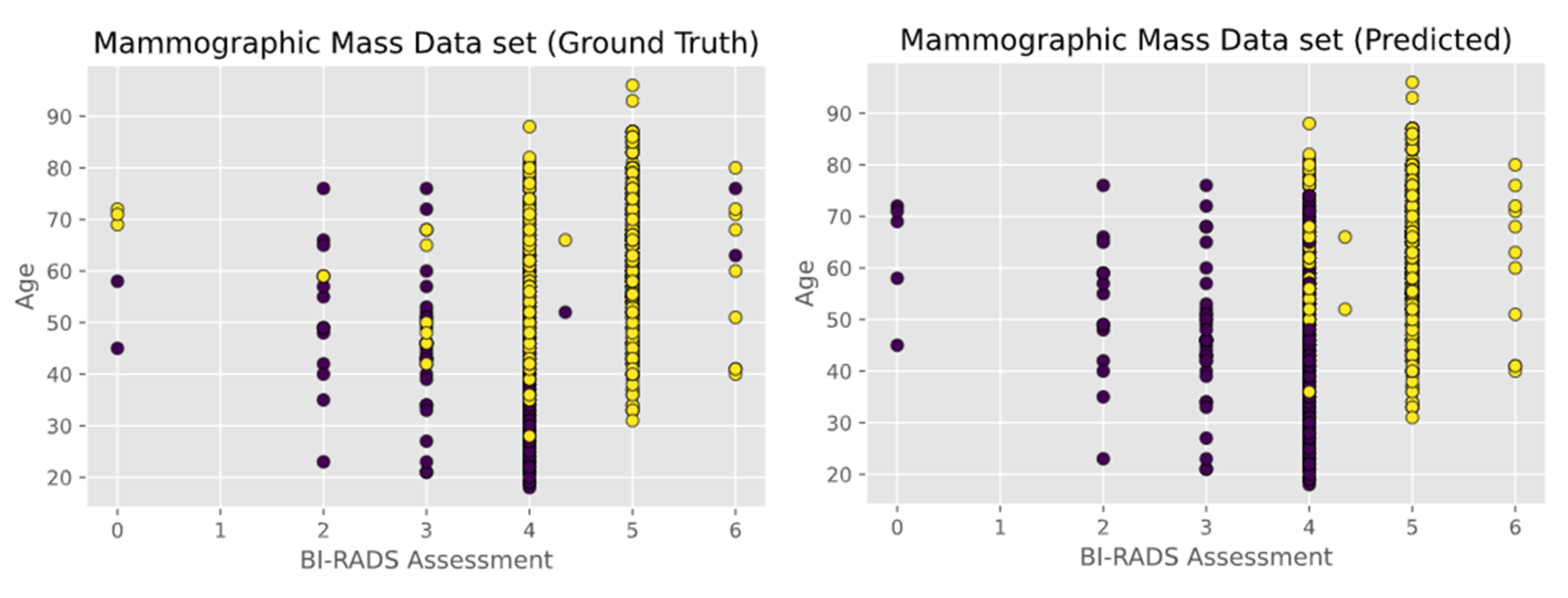
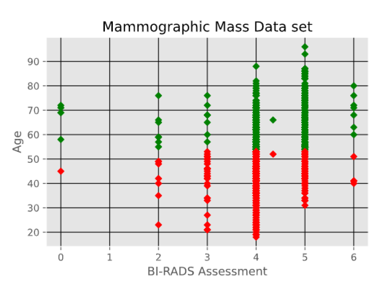
- Mammographic Mass data set containing 961 instances and is used to classify data into two categories, benign and malignant. Each instance contains 6 attributes based on BI-RADS data and the patient’s age. The attributes are as follows: BI-RADS assessment, age, shape, margin, density, and severity. The first two attributes i.e., BI-RADS Assessment and Age are shown in Figure 6.
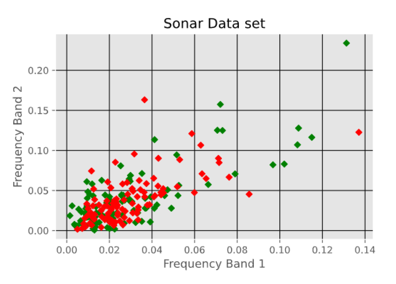
- 5.
- Sonar Data set, which consists of 208 instances with 60 attributes each. The instances are classified into either mines or rocks. The attributes represent the energy within a specific frequency band. The first two attributes i.e. Frequency Band 1 and Frequency Band 2 are shown in Figure 7.
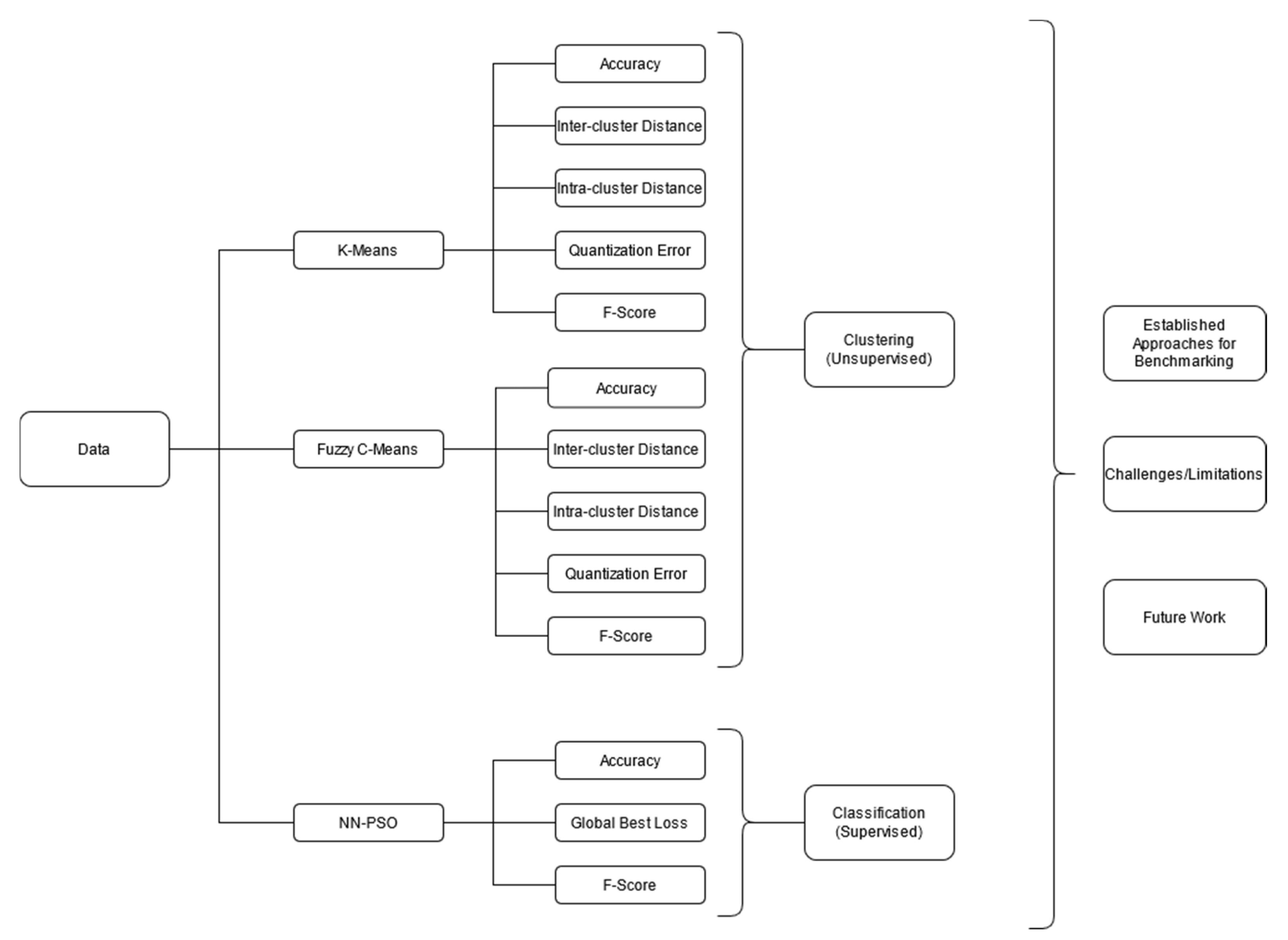
3.3. Performance Indices
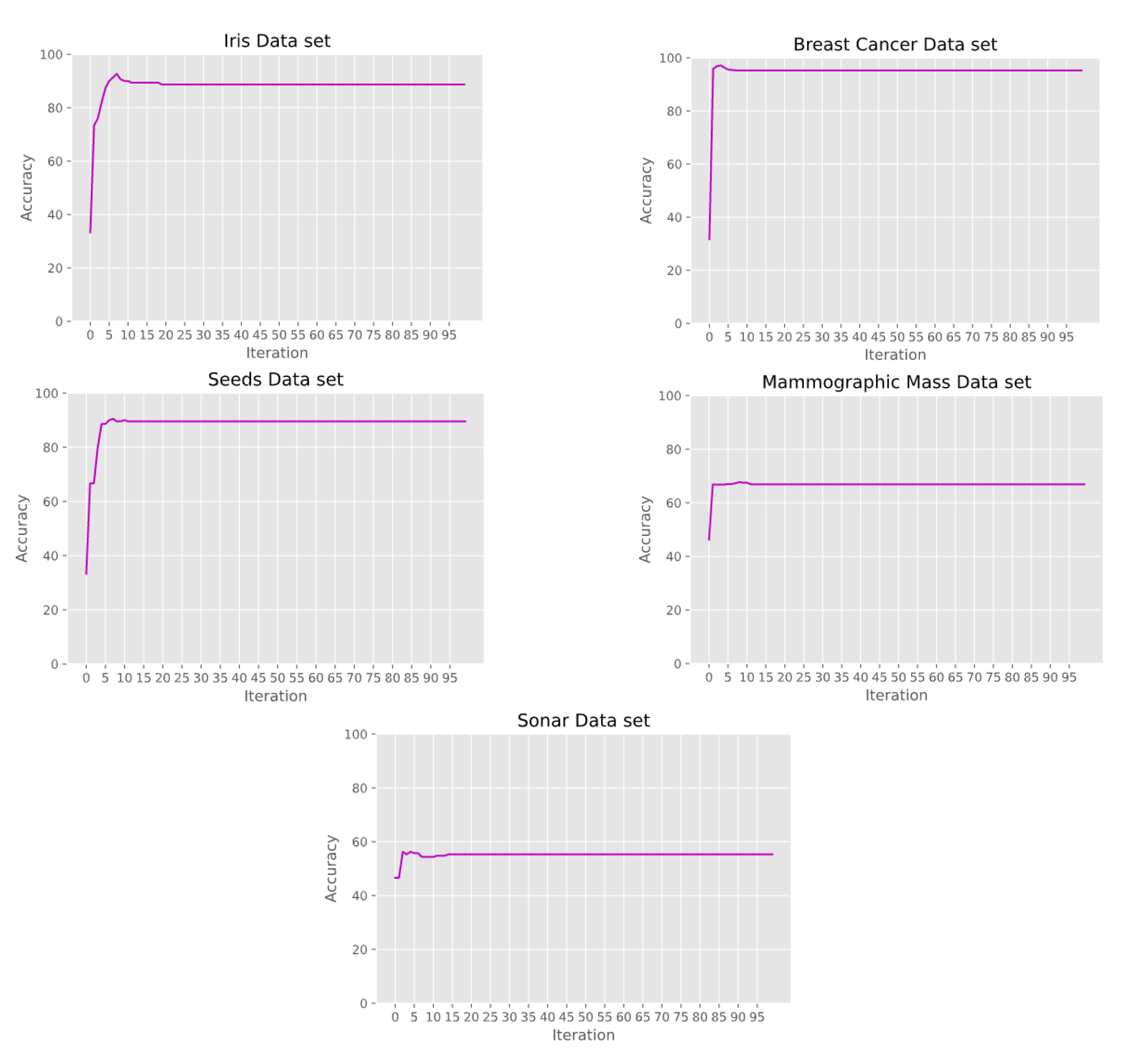
- Accuracy: This is also known as the Rand index. The accuracy is described as the percentage of correct decisions made by the algorithm. The formula for accuracy is as follows:
- F-Score: Another means of calculating accuracy. It is calculated using the precision and recall of a model the formula for F-Score is as follows:
- Inter-Cluster Distance: The sum of the distances between each cluster centroid. Larger values indicate a greater separation between clusters, meaning less overlap between the clusters in the model. The formula for inter-cluster distance is as follows [34]:where represents the centroid of cluster .
- Intra-Cluster Distance: The sum of the distances between individual data points and their respective parent centroid. Smaller values indicate more compact clusters and are therefore desired. The formula for intra-cluster distance is as follows [34]:is the number of clusters, represents the centroid , and refers to the number of data instances. The section represents the distance between data instances and their respective centroid.
- Quantization Error: The sum of the distances between data points and their parent centroid divided by the total number of data points belonging to the cluster and then summed over all clusters and averaged for all of the clusters in the model. The formula for quantization error is as follows [34]:
3.4. K-Means Implementation
Trapping in Local Optima
3.5. Fuzzy C-Means Implementation
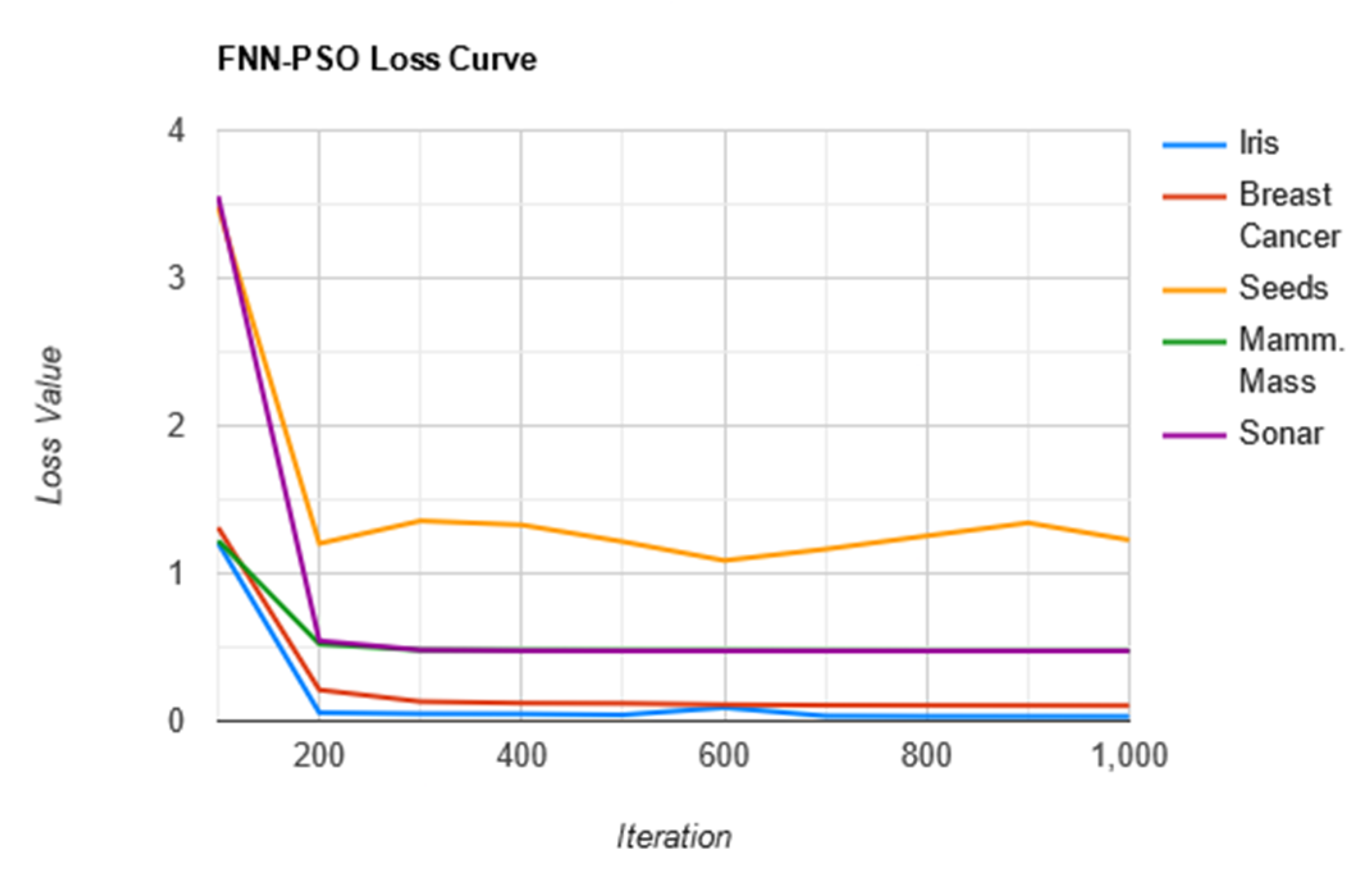
3.6. Feed-Forward Neural Network Tuned by a Particle Swarm Optimization Algorithm
4. Results and Related Discussion
5. Concluding Remarks and Observations from Related Studies
5.1. Related Work and Performance
- “Comparative Analysis of K-means and K-medoids Algorithm on IRIS Data” [35], authored by Kalpit G. Soni and Atul Patel.
- “Self-organizing Maps as Substitutes for K-Means Clustering” [36], authored by Fernando Bação, Victor Lobo, and Marco Painho.
- “Comparison of Machine Learning Methods for Breast Cancer Diagnosis” [37], authored by Ebru Aydındag Bayrak, Pınar Kırcı and Tolga Ensari.
- “Ensemble Decision Tree Classifier for Breast Cancer Data” [38], authored by D. Lavanya and K. Usha Rani.
- “An Application of Deep Neural Network for Classification of Wheat Seeds” [39], authored by Ayşe Eldem.
- “Predicting breast cancer biopsy outcomes from BI-RADS findings using random forests with chi-square and MI features” [40], authored by Sheldon Williamson, K. Vijayakumar, and Vinod J. Kadam.
- “Classification of Sonar Targets Using OMKC, Genetic Algorithms and Statistical Moments” [41], authored by Mohammad Reza Mosavi, Mohammad Khishe, Ehsan Ebrahimi.
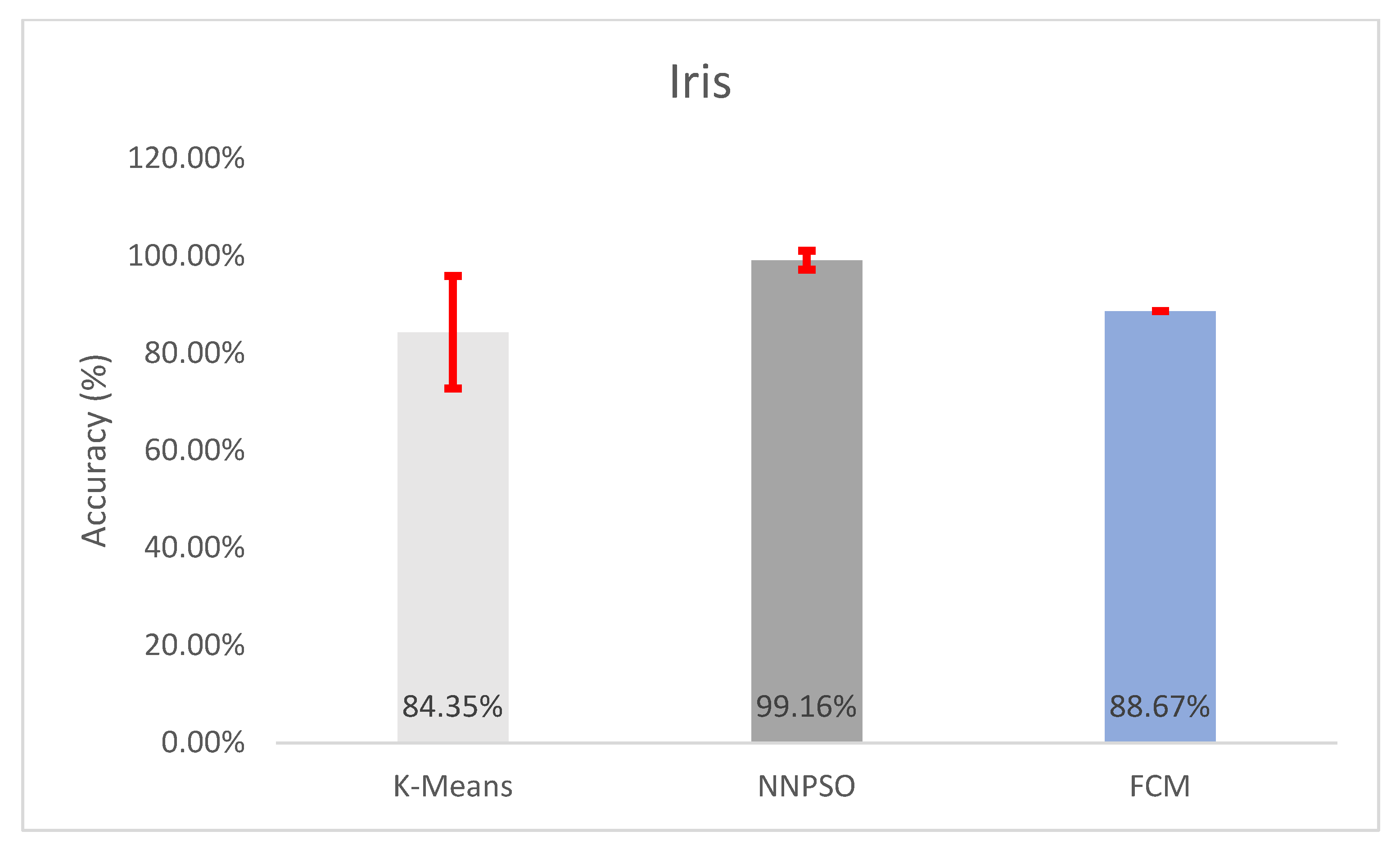
5.2. Observations on Iris
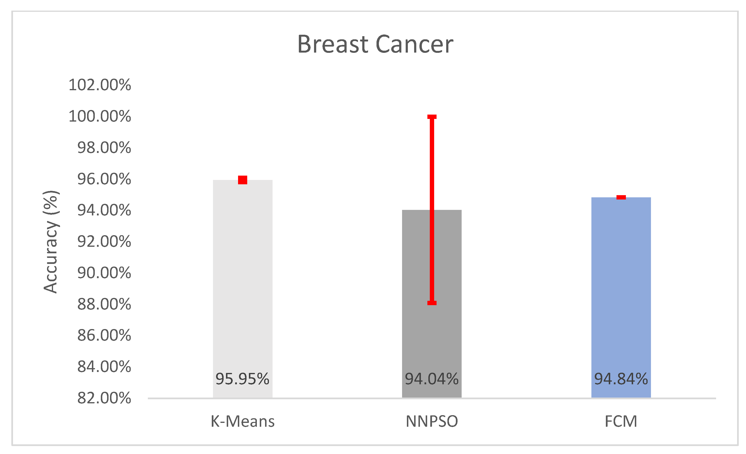
5.3. Observations on Breast Cancer
5.4. Observations on Seeds
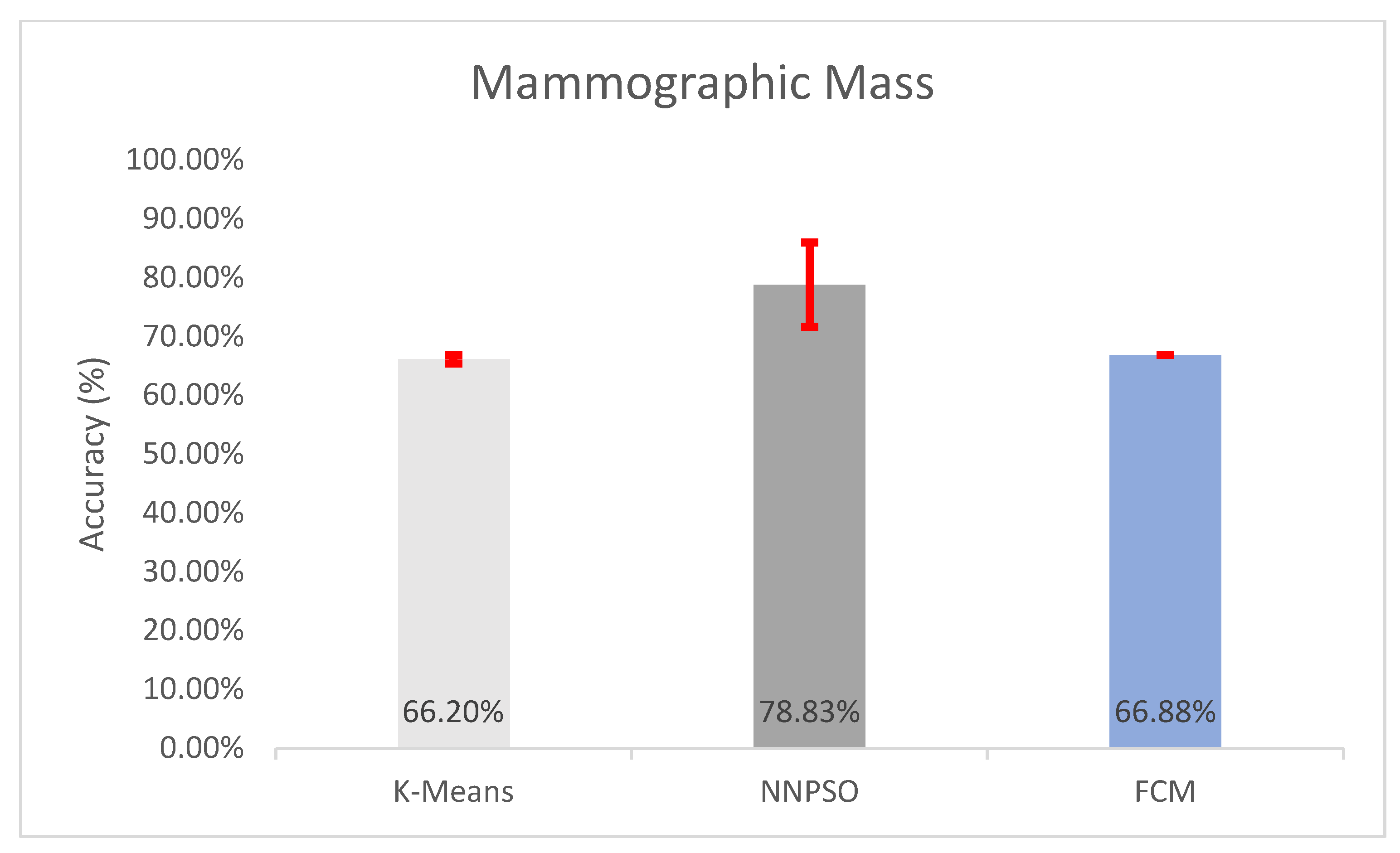
5.5. Observations on Mammographic Mass
5.6. Observations on Sonar
Author Contributions
Funding
Institutional Review Board Statement
Informed Consent Statement
Data Availability Statement
Acknowledgments
Conflicts of Interest
References
- Ahmadyfard, A.; Modares, H. Combining PSO and k-means to enhance data clustering. In Proceedings of the 2008 International Symposium on Telecommunications, Tehran, Iran, 27–28 August 2008; pp. 688–691. [Google Scholar]
- Sengupta, S.; Basak, S.; Peters, R.A. Data clustering using a hybrid of fuzzy c-means and quantum-behaved particle swarm optimization. In Proceedings of the 2018 IEEE 8th Annual Computing and Communication Workshop and Conference (CCWC), Las Vegas, NV, USA, 8–10 January 2018; pp. 137–142. [Google Scholar]
- Sengupta, S.; Basak, S.; Saikia, P.; Paul, S.; Tsalavoutis, V.; Atiah, F.; Ravi, V.; Peters, A. A review of deep learning with special emphasis on architectures, applications and recent trends. Knowl. Based Syst. 2020, 194, 105596. [Google Scholar] [CrossRef] [Green Version]
- Merwe, D.W.; Engelbrecht, A.P. Data Clustering Using Particle Swarm Optimization. In Proceedings of the 2003 Congress on Evolutionary Computation, Canberra, Australia, 8–12 December 2003; pp. 215–220. [Google Scholar]
- MacQueen, J. Some methods for classification and analysis of multivariate observations. In Proceedings of the Fifth Berkeley Symposium on Mathematical Statistics and Probability, Berkeley, CA, USA, 21 June–18 July 1965; Volume 1, pp. 281–297. [Google Scholar]
- Tarkhaneh, O.; Shen, H. Training of feedforward neural networks for data classification using hybrid particle swarm optimization, Mantegna Lévy flight and neighborhood search. Heliyon 2019, 5, e01275. [Google Scholar] [CrossRef] [Green Version]
- Zhang, C.; Shao, H. Particle Swarm Optimisation in Feedforward Neural Network. In Artificial Neural Networks in Medicine and Biology. Perspectives in Neural Computing; Malmgren, H., Borga, M., Niklasson, L., Eds.; Springer: London, UK, 2000. [Google Scholar] [CrossRef]
- Karaboga, D.; Akay, B.; Ozturk, C. Artificial Bee Colony (ABC) Optimization Algorithm for Training Feed-Forward Neural Networks. In Modeling Decisions for Artificial Intelligence; Torra, V., Narukawa, Y., Yoshida, Y., Eds.; MDAI 2007. Lecture Notes in Computer Science; Springer: Berlin/Heidelberg, Germany, 2017; Volume 4617. [Google Scholar] [CrossRef]
- Kennedy, J.; Eberhart, R. Particle swarm optimization. In Proceedings of the ICNN’95-International Conference on Neural Networks, Perth, WA, Australia, 27 November–1 December 1995; Volume 4, pp. 1942–1948. [Google Scholar]
- Karaboga, D.; Basturk, B. A powerful and efficient algorithm for numerical function optimization: Artificial bee colony (ABC) algorithm. J. Glob. Optim. 2007, 39, 459–471. [Google Scholar] [CrossRef]
- Sengupta, S.; Basak, S.; Peters, R.A. QDDS: A Novel Quantum Swarm Algorithm Inspired by a Double Dirac Delta Potential. In Proceedings of the 2018 IEEE Symposium Series on Computational Intelligence (SSCI), Bangalore, India, 18–21 November 2018; pp. 704–711. [Google Scholar] [CrossRef] [Green Version]
- Yang, X.S.; Deb, S. Cuckoo Search via Lévy flights. In Proceedings of the 2009 World Congress on Nature & Biologically Inspired Computing (NaBIC), Coimbatore, India, 9–11 December 2009; pp. 210–214. [Google Scholar]
- Colorni, A.; Dorigo, M.; Maniezzo, V. Distributed Optimization by Ant Colonies. In Actes de la Première Conférence Européenne sur la vie Artificielle, Paris, France; Elsevier Publishing: Amsterdam, The Netherlands, 1991; pp. 134–142. [Google Scholar]
- Sengupta, S.; Basak, S.; Peters, R.A., II. Chaotic Quantum Double Delta Swarm Algorithm Using Chebyshev Maps: Theoretical Foundations, Performance Analyses and Convergence Issues. J. Sens. Actuator Netw. 2019, 8, 9. [Google Scholar] [CrossRef] [Green Version]
- Sha, D.; Lin, H.-H. A multi-objective PSO for job-shop scheduling problems. Expert Syst. Appl. 2010, 37, 1065–1070. [Google Scholar] [CrossRef]
- Chen, C.; Zhou, K. Application of Artificial Bee Colony Algorithm in Vehicle Routing Problem with Time Windows. In Proceedings of the 2018 International Conference on Sensing, Diagnostics, Prognostics, and Control (SDPC), Xi’an, China, 15–17 August 2018; pp. 781–785. [Google Scholar] [CrossRef] [Green Version]
- Marinakis, Y.; Marinaki, M.; Migdalas, A. Particle Swarm Optimization for the Vehicle Routing Problem: A Survey and a Comparative Analysis. In Handbook of Heuristics; Martí, R., Pardalos, P., Resende, M., Eds.; Springer: Cham, Switzerland, 2018. [Google Scholar]
- Sengupta, S.; Basak, S. Computationally efficient low-pass FIR filter design using Cuckoo Search with adaptive Levy step size. In Proceedings of the 2016 International Conference on Global Trends in Signal Processing, Information Computing and Communication (ICGTSPICC), Jalgaon, India, 22–24 December 2016; pp. 324–329. [Google Scholar] [CrossRef]
- Dhabal, S.; Sengupta, S. Efficient design of high pass FIR filter using quantum-behaved particle swarm optimization with weighted mean best position. In Proceedings of the 2015 Third International Conference on Computer, Communication, Control and Information Technology (C3IT), Hooghly, India, 7–8 January 2015; pp. 1–6. [Google Scholar] [CrossRef]
- Zhu, H.; Wang, Y.; Wang, K.; Chen, Y. Particle Swarm Optimization (PSO) for the constrained portfolio optimization problem. Expert Syst. Appl. 2011, 38, 10161–10169. [Google Scholar] [CrossRef]
- Kumar, D.; Mishra, K. Portfolio optimization using novel co-variance guided Artificial Bee Colony algorithm. Swarm Evol. Comput. 2017, 33, 119–130. [Google Scholar] [CrossRef]
- Basak, S.; Sun, F.; Sengupta, S.; Dubey, A. Data-Driven Optimization of Public Transit Schedule. In Big Data Analytics; Madria, S., Fournier-Viger, P., Chaudhary, S., Reddy, P., Eds.; BDA 2019. Lecture Notes in Computer Science; Springer: Cham, Switzerland, 2019; Volume 11932. [Google Scholar] [CrossRef] [Green Version]
- Majhi, S.K.; Biswal, S. Optimal cluster analysis using hybrid K-Means and Ant Lion Optimizer. Karbala Int. J. Mod. Sci. 2018, 4, 347–360. [Google Scholar] [CrossRef]
- K-Means Advantages and Disadvantages|Clustering in Machine Learning. 2021. Available online: https://developers.google.com/machine-learning/clustering/algorithm/advantages-disadvantages (accessed on 10 February 2021).
- Nayak, J.; Naik, B.; Behera, H.S. Fuzzy C-Means (FCM) Clustering Algorithm: A Decade Review from 2000 to 2014. Blockchain Technol. Innov. Bus. Process. 2015, 2, 133–149. [Google Scholar]
- Bezdek, J.C. Modified Objective Function Algorithms. In Pattern Recognition with Fuzzy Objective Function Algorithms; Springer US Science & Business Media: New York, NY, USA, 1981; pp. 155–201. [Google Scholar]
- Torra, V. On Fuzzy c -Means and Membership Based Clustering. In International Work-Conference on Artificial Neural Networks; Springer: Cham, Switzerland, 2015; pp. 597–607. [Google Scholar]
- Zhang, J.; Ma, Z. Hybrid Fuzzy Clustering Method Based on FCM and Enhanced Logarithmical PSO (ELPSO). Comput. Intell. Neurosci. 2020, 2020, 1–12. [Google Scholar] [CrossRef] [PubMed] [Green Version]
- Feng, Y.; Lu, H.; Xie, W.; Yin, H.; Bai, J. An Improved Fuzzy C-Means Clustering Algorithm Based on Multi-chain Quantum Bee Colony Optimization. Wirel. Pers. Commun. 2017, 102, 1421–1441. [Google Scholar] [CrossRef]
- Figueiredo, E.M.; Ludermir, T. Investigating the use of alternative topologies on performance of the PSO-ELM. Neurocomputing 2014, 127, 4–12. [Google Scholar] [CrossRef]
- Sengupta, S.; Basak, S.; Peters, R. Particle Swarm Optimization: A Survey of Historical and Recent Developments with Hybridization Perspectives. Mach. Learn. Knowl. Extr. 2018, 1, 10. [Google Scholar] [CrossRef] [Green Version]
- UCI Machine Learning Repository. Available online: http://archive.ics.uci.edu/ml/ (accessed on 10 February 2021).
- Scikit-learn Library. Available online: https://scikit-learn.org/stable/ (accessed on 10 February 2021).
- Patel, G.K.; Dabhi, V.K.; Prajapati, H.B. Clustering Using a Combination of Particle Swarm Optimization and K-means. J. Intell. Syst. 2016, 26, 457–469. [Google Scholar] [CrossRef]
- Soni, K.G.; Patel, A. Comparative Analysis of K-means and K-medoids Algorithm on IRIS Data. Int. J. Comput. Intell. Res. 2017, 13, 899–906. [Google Scholar]
- Bação, F.; Lobo, V.; Painho, M. Self-organizing Maps as Substitutes for K-Means Clustering. In Computational Science–ICCS 2006; Springer: Berlin/Heidelberg, Germany, 2005; pp. 476–483. [Google Scholar] [CrossRef] [Green Version]
- Bayrak, E.A.; Kirci, P.; Ensari, T. Comparison of Machine Learning Methods for Breast Cancer Diagnosis. In Proceedings of the 2019 Scientific Meeting on Electrical-Electronics & Biomedical Engineering and Computer Science (EBBT), Istanbul, Turkey, 24–26 April 2019. [Google Scholar] [CrossRef]
- Lavanya, D.; Rani, K.U. Ensemble Decision Making System for Breast Cancer Data. Int. J. Comput. Appl. 2012, 51, 19–23. [Google Scholar] [CrossRef]
- Eldem, A. An Application of Deep Neural Network for Classification of Wheat Seeds. Avrupa Bilim Ve Teknol. Derg. 2020, 19, 213–220. [Google Scholar]
- Williamson, S.; Vijayakumar, K.; Kadam, V.J. Predicting breast cancer biopsy outcomes from BI-RADS findings using random forests with chi-square and MI features. Multimed. Tools Appl. 2021, 1–21. [Google Scholar] [CrossRef]
- Mosavi, M.R.; Khishe, M.; Ebrahimi, E. Classification of sonar targets using OMKC, genetic algorithms and statistical moments. J. Adv. Comput. Res. 2016, 7, 143–156. [Google Scholar]
- Hanif, M. Parallelized PSO Clustering; GitHub Repository. 2020. Available online: https://github.com/ms03831/parallelized-PSO-clustering (accessed on 10 February 2021).
- Shriti, K. Fuzzy C Means Clustering; GitHub Repository. 2020. Available online: https://github.com/ShristiK/Fuzzy-C-Means-Clustering (accessed on 10 February 2021).
- Ahmad, Z. Train Neural Network (Numpy)-Particle Swarm Optimization (PSO). 2020. Available online: https://medium.com/@zeeshanahmad10809/train-neural-network-numpy-particle-swarm-optimization-pso-93f289fc8a8e (accessed on 10 February 2021).
- Prateekk94. Fuzzy C-Means Clustering on Iris Dataset. 2020. Available online: https://www.kaggle.com/prateekk94/fuzzy-c-means-clustering-on-iris-dataset (accessed on 10 February 2021).


| Data Set | Inertia Weight Range | Cognitive Factor | Social Factor |
|---|---|---|---|
| Iris | 0.7–0.9 | 0.5 | 0.7 |
| Breast Cancer | 0.9–0.9 | 0.4 | 0.1 |
| Seeds | 0.7–0.9 | 0.9 | 0.1 |
| Mammographic Mass | 0.6–0.9 | 0.1 | 0.9 |
| Sonar | 0.9–0.9 | 0.2 | 0.1 |
| Number of Instances | Number of Attributes | Number of Categories | |
|---|---|---|---|
| Iris | 150 | 4 | 3 |
| Breast Cancer | 699 | 10 | 2 |
| Seeds | 210 | 7 | 3 |
| Mammographic Mass | 961 | 6 | 2 |
| Sonar | 208 | 60 | 2 |
| Data | Accuracy | Inter Cluster Distance | Intra Cluster Distance | Quantization Error | F-Score |
|---|---|---|---|---|---|
| Iris | 84.3467 ± 11.5433% | 9.9448 ± 0.5077 | 100.9036 ± 9.1452 | 0.6525 ± 0.0174 | 0.8435 ± 0.1154 |
| Breast Cancer | 95.9484 ± 0.1393% | 27.5215 ± 0.0287 | 3050.4339 ± 1.2969 | 5.2425 ± 0.0069 | 0.9595 ± 0.0014 |
| Seeds | 89.2952 ± 0.2379% | 15.9245 ± 0.1182 | 313.4652 ± 0.2585 | 1.4967 ± 0.0003 | 0.893 ± 0.0024 |
| Mammographic Mass | 66.2042 ± 0.7268% | 47.8242 ± 0.2174 | 6993.7479 ± 10.2771 | 7.2945 ± 0.0048 | 0.662 ± 0.0073 |
| Sonar | 52.6442 ± 3.7956% | 2.5068 ± 0.0124 | 235.1373 ± 0.4677 | 1.127 ± 0.0056 | 0.5264 ± 0.038 |
| Data | Accuracy | Inter-Cluster Distance | Intra-Cluster Distance | Quantization Error | F-Score |
|---|---|---|---|---|---|
| Iris | 88.6667 ± 1.1102e-14% | 9.994 ± 3.7006e-15 | 96.9562 ± 2.309e-14 | 0.646 ± 9.5505e-17 | 0.8867 ± 1.1102e-16 |
| Breast Cancer | 94.8424 ± 2.2204e-14% | 26.9631 ± 7.4012e-15 | 2681.0984 ± 4.5475e-13 | 4.7631 ± 1.2243-15 | 0.9484 ± 2.2204e-16 |
| Seeds | 89.5238 ± 1.1102e-14% | 16.1425 ± 1.4921e-14 | 312.5735 ± 4.9555e-14 | 1.4936 ± 1.3688e-16 | 0.8952 ± 1.1102e-16 |
| Mammographic Mass | 66.875 ± 2.2204e-14% | 48.7586 ± 0.572e-14 | 7023.1509 ± 5.2389e-12 | 7.3333 ± 4.432e-15 | 0.6687 ± 2.2204e-16 |
| Sonar | 55.2885 ± 0.0000% | 1.8598 ± 1.1508e-14 | 237.3494 ± 4.5848e-13 | 1.139 ± 1.9135e-15 | 0.5529 ± 0.0000 |
| Data | Accuracy | Global Best Loss | F-Score |
|---|---|---|---|
| Iris | 99.1556 ± 1.9317% | 0.0481 ± 0.0353 | 0.9916 ± 0.0193 |
| Breast Cancer | 94.0381 ± 5.9493% | 0.1541 ± 0.109 | 0.9404 ± 0.0595 |
| Seeds | 81.7143 ± 7.4872% | 0.4653 ± 0.0995 | 0.8171 ± 0.0749 |
| Mammographic Mass | 78.8264 ± 7.1728% | 0.4864 ± 0.0638 | 0.7883 ± 0.0717 |
| Sonar | 71.2666 ± 8.492% | 0.546 ± 0.0809 | 0.7127 ± 0.0849 |
Publisher’s Note: MDPI stays neutral with regard to jurisdictional claims in published maps and institutional affiliations. |
© 2021 by the authors. Licensee MDPI, Basel, Switzerland. This article is an open access article distributed under the terms and conditions of the Creative Commons Attribution (CC BY) license (https://creativecommons.org/licenses/by/4.0/).
Share and Cite
Pickens, A.; Sengupta, S. Benchmarking Studies Aimed at Clustering and Classification Tasks Using K-Means, Fuzzy C-Means and Evolutionary Neural Networks. Mach. Learn. Knowl. Extr. 2021, 3, 695-719. https://doi.org/10.3390/make3030035
Pickens A, Sengupta S. Benchmarking Studies Aimed at Clustering and Classification Tasks Using K-Means, Fuzzy C-Means and Evolutionary Neural Networks. Machine Learning and Knowledge Extraction. 2021; 3(3):695-719. https://doi.org/10.3390/make3030035
Chicago/Turabian StylePickens, Adam, and Saptarshi Sengupta. 2021. "Benchmarking Studies Aimed at Clustering and Classification Tasks Using K-Means, Fuzzy C-Means and Evolutionary Neural Networks" Machine Learning and Knowledge Extraction 3, no. 3: 695-719. https://doi.org/10.3390/make3030035