Optimization and Prediction of Thermal Conductivity and Electrical Conductivity of Vacuum Sintered Ti-6Al-4V-SiC(15 Wt.%) Using Soft Computing Techniques

Abstract

Titanium silicon carbide (Ti₃SiC₂) is a novel composite material that has found a multitude of uses in the aerodynamics, automobile, and marine industries due to its excellent properties such as high strength and modulus, high thermal and electrical conductivity, high melting point, excellent corrosion resistance, and high-temperature oxidation resistance. These properties are strongly associated with physical properties and microstructural features. Due to difficulties in the synthesis of this material, there have been very few investigations on the relationship between microstructure and physical characteristics of titanium silicon carbide composites processed through powder metallurgical process. However, the importance of thermal conductivity and electrical conductivity of titanium silicon carbide composites in various potential applications has led to keen attention from several researchers. Hence, in this paper, optimization, and prediction of process input parameters during processing under vacuum sintering for achieving maximum electrical and thermal conductivity of Ti-6Al-4V-SiC(15 Wt.%) has been presented. Using Taguchi’s L₉ Orthogonal Array, it has been observed that aging temperature (1150 °C), aging time (four hours), heating rate (25 °C/min), and cooling rate (5 °C/min) result in optimum input parameters for achieving the highest electrical conductivity values during the processing of Ti-6Al-4V-SiCp composites. Further, for maximum thermal conductivity values during the processing of Ti-6Al-4V-SiCp composites, aging temperature (1150 °C), aging time (four hours), heating rate (5 °C/min), and cooling rate (5 °C/min) are preferred. A second-order response surface model generated can be effectively used for predicting the electrical conductivity and thermal conductivity during the processing of Ti-6Al-4V-SiCp composites with an accuracy of 99.28% (electrical conductivity) and 99.14% (thermal conductivity). By comparing the experimental results along with the results of the mathematical model and the BPANN model results for nine trials, it was observed that the estimated value is accurate for all tests with an error of 0.39% (electrical conductivity) and 0.48% (thermal conductivity). Further, from X-ray diffraction studies and microstructural analysis, it has been observed that aging at 1150 °C for four hours resulted in the formation of a ternary carbide phase of titanium silicon carbide (Ti₃SiC₂), which resulted in maximum electrical conductivity (4,260,000 Ω⁻¹ m⁻¹) and thermal conductivity (36.42 W/m·K) of the Ti-6Al-4V-SiC (15 Wt.%) composite specimen.

1. Introduction

Titanium silicon carbide (Ti₃SiC₂) is a novel composite material that has found a multitude of uses in the aerodynamics, machining, and marine industries due to its excellent properties such as high strength and modulus, high thermal and electrical conductivity, high melting point, excellent corrosion resistance, and high-temperature oxidation resistance. These properties are strongly associated with physical properties and microstructure features. Due to difficulties in the synthesis of this material, there have been very few investigations on the relationship between microstructure and physical characteristics. Titanium silicon carbide (Ti₃SiC₂) has attracted a lot of attention in the last ten years as a “representative compound of the ternary Mn+1AXn phases (or MAX phases)”, where M is denoted as metal that transitions early with examples like Ti, Cr, Al, and Si, X is denoted by either carbon or nitrogen (some exceptions with both carbon and nitrogen), and n represents a number (1,2,3, etc) [1,2,3]. Its crystal structure consists of three relatively tightly packed Ti layers that contain C atoms in the octahedral positions between three hexagonal nets of Si atoms [4]. This material, which has a density of 4.52 g/cm³, is a potential material for structural and functional materials used in high-temperature applications. It has a hardness value of HV 4 GPa, making it comparatively soft with a strong thermal shock resistance [1]. The first account of the synthesis of Ti₃SiC₂ via chemical reaction was noted in 1967 by Jeitschko and Nowotny [5]. Goto and Hirai [4] analyzed the processing of Ti₃SiC₂ following the(CVD) chemical vapor deposition route in 1987. Barsoum et al. (2,3) successfully processed a composite material with a relatively high Ti₃SiC₂ content (almost 98 vol%) from mixtures of Ti-SiC-C following the hot-isostatic pressing (HIP) method.

Few other examples of Ti/Si/C and Ti/Si/TiC combinations were produced successfully using the HIP approach or other techniques [6,7,8,9,10,11,12]. However, the current sintering methods were frequently carried out for extended periods at a high temperature (1400–1600 °C). For the quick reactive sintering of ceramics and intermetallic materials, a novel method known as pulse discharge sintering (PDS), sometimes known as spark plasma sintering (SPS), was employed [13]. Particularly at high temperatures, titanium can potentially benefit greatly from ceramic reinforcement in terms of its mechanical properties. The difficulties of preventing an interfacial chemical reaction, either during manufacturing or in applications, which is known to damage the mechanical properties, especially if its thickness is greater than roughly one micron, is a main concern among researchers. Though properties like thermal conductivity and thermal expansivity are crucial in defining the thermal shock resistance and other qualities related to use at high temperatures, relatively few studies have been conducted to analyze the thermal and electrical properties of Ti-SiC and Ti-Ti.B2 composites processed through the powder metallurgical route. Several authors have emphasized the significance of electrical and thermal conductivity for metal-matrix composites (MMCS) in various prospective applications [14,15,16,17,18]. From both the practical and theoretical perspectives, the thermal characteristics of SiC/Ti and TiB2/Ti are of great interest due to their improved thermal and electrical conductivity compared to the majority of reference data showing that these ceramics have a higher conductivity than titanium. As phonons, which are easily scattered by defects, are the only mode of heat transfer in SiC and TiB2, the thermal conductivity of these materials is strongly dependent on structural elements such as grain size and porosity. Furthermore, heat must be transported across the matrix–reinforcement interface to improve (or even retain) the matrix thermal conductivity in a composite. Very little research has been conducted to understand the effectiveness of this occurrence in MMCs, where transport is often mostly accomplished by phonons in the ceramic and electrons in the matrix. The size of the reinforcing inclusion should also be taken into account. In addition to the expected increase in phonon scattering at boundaries with small entities, it is evident that bigger reinforcement will result in less frequent displacement of heat, as it is transmitted through a composite material [19]. Hence, in this paper, the optimization and prediction of process input parameters during processing under vacuum sintering for achieving the maximum electrical and thermal conductivity of Ti-l-4V-SiC (15 Wt.%) have been presented. The prime objective of this research is to establish the favorable vacuum sintering process parameters for Ti-6Al-4V-SiC (15 Ti-6Al-4V-SiC (15Wt.%) composites under different aging temperature (°C), aging time (h), heating rate (°C/min) and cooling rate (°C/min) to maximize the electrical conductivity and thermal conductivity using Taguchi’s L₉ orthogonal array. Further, response surface methodology and back propagation artificial neural networks have been used to predict the optimum process input parameters. Finally, microstructure analysis along with X-ray diffraction confirms the formation of ternary carbide phase (Ti₃SiC₂) which increased the electrical and thermal conductivity of Ti-6Al-4V-SiC (15 Wt.%) composites, has also been discussed.

2. Methodology

In this experiment, silicon carbide (SiC) with a particle size of 100 microns was employed as a reinforcement in a titanium alloy (Ti-6Al-4V) matrix. The processing flowchart for the titanium silicon carbide composite employed in this investigation is shown in Figure 1.

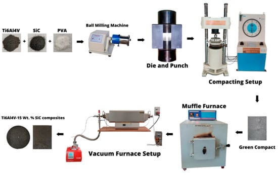
Figure 1. Flowchart of Titanium Silicon Carbide composite processing [20].

Table 1, Table 2, Table 3 and Table 4 exhibit the chemical composition, mechanical, and thermal characteristics of silicon carbide and titanium alloy, respectively. The powders were blended using a planetary ball mill followed by compaction using custom-manufactured dies. Green titanium silicon carbide composites were vacuum sintered utilizing an RHTC 80-710/15 HTV high-temperature vacuum sintering machine after being pre-sintered at 500 °C in a muffle furnace to vaporize binder material. The vacuum sintering process was carried out under various conditions, such as aging temperature (°C), aging time (h), heating rate (°C/min), and cooling rate (°C/min) [20].

Table 1. Composition (Wt%) of Ti-6Al-4V alloy [20].

Element	Aluminium	Vanadium	Iron	Oxygen	Carbon	Nitrogen	Titanium
Wt (%)	6.1063	4.103	0.1675	0.1124	0.0235	0.0193	Balance

Table 2. Composition (Wt%) of SiC reinforcement particle [20].

Element	Carbon	Iron	Nitrogen	Aluminum	Calcium	Oxygen	Potassium	Silicon
Wt (%)	1.172	0.664	1.4353	0.2557	0.1454	0.8642	0.3243	Balance

Table 3. Thermal properties and Mechanical Properties of Ti-6Al-4V alloy [20].

Properties	Values (Units)
Density	4.43 g/cm3
Melting Point	1604–1660 °C
Beta Transitional Temperature	980 °C
Tensile Strength, Ultimate	1170 Mpa
Tensile Strength, Yield	1100 Mpa
Compressive Strength	1070 Mpa
Modulus of Elasticity	114 Gpa
Brinell Hardness	379 BHN

Table 4. Thermal properties and Mechanical Properties of SiC [20].

Properties	Values (Units)
Density	3.1 g/cm3
Melting Point	2730 °C
Beta Transitional Temperature	2000 °C
Tensile Strength, Ultimate	390 Mpa
Compressive Strength	2000 Mpa
Modulus of Elasticity	410 Gpa
Vicker’s Hardness	2720 Hv

The electrical conductivity of the Ti-6Al-4V-SiC(15 Wt.%) sample of size 20 × 10 × 2 mm (Figure 2) was measured using a Keith 400 low-temperature resistivity measuring instrument (Figure 3).

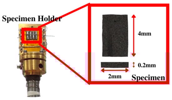
Figure 2. Workpiece for measuring electrical conductivity.

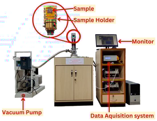
Figure 3. Keith 400 low-temperature electrical resistivity measuring instrument.

The four probes have been attached to the sample using thermal paste at an interval of 5mm each and placed inside the vacuum chamber. The temperature is increased to 360 °C and decreased to 10 °C while the values of voltage (V) versus current (I) are recorded using a data acquisition system. Resistivity was calculated using Equation (1). Further, electrical conductivity was measured using Equation (2).

$$\rho =\frac{V}{I}\frac{\pi t}{ln\frac{sinh\frac{t}{s}}{sinh\frac{t}{2s}}}$$

(1)

where,

• ρ = Resistivity of the sample,
• V = voltage,
• I = current,
• t = thickness of the sample,
• s = distance between the probes

$$\sigma =\frac{1}{\rho }$$

(2)

where,

• σ = electrical conductivity of the sample.

For thermal conductivity, a Ti-6Al-4V-SiC(15 Wt.%) composite material of diameter 12.7 mm and thickness 5mm (Figure 4) was analyzed using ‘DLF-2™, Waters, Austria’ laser flash thermal analysis system (Figure 5).

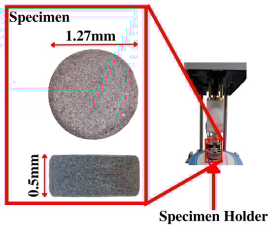
Figure 4. Workpiece for measuring thermal conductivity.

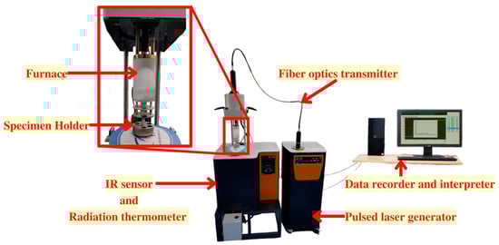
Figure 5. LASER flash thermal analysis system.

In this procedure, a laser-generated very brief pulse of energy was used to evenly irradiate the specimen’s front face up to the desired temperature range. The sample’s thermal diffusivity was calculated using the time-dependent thermograph of the back face. Thermal diffusivity along with specific heat capacity was measured for a temperature range of 30 °C to 1000 °C with the machine-specified error of ⁺/₋ 2%. Thermal diffusivity is related to thermal conductivity as shown in Equation (3).

$$\mathrm{Thermal}\mathrm{Diffusivity}\alpha =\frac{k}{\rho C_p}$$

(3)

where,

• k = thermal conductivity;
• ρ = density;
• C_p = specific heat capacity.

To find the ideal process input parameters, Taguchi’s L₉ orthogonal array was used. Further, this experiment employs response surface methodology to predict the process output parameters using a second-order equation. Powder X-ray diffraction analysis of sintered Ti-6Al-4V-SiC (15 Wt.%) composite powders was performed using Rigaku Miniflex 600 X-ray Diffractometer for 0–80° 2θ value. Microstructure and elemental mapping of the samples were conducted using an Olympic System Optical Microscope and an EVO MA18 Scanning Electron Microscope with Oxford EDS (X-act).

2.1. Taguchi’s Design of Experiments (TDOE)

Engineering applications frequently use the Taguchi design of experiments to attain the highest values of quality attributes under various circumstances. Users with little statistical understanding can easily adapt and use Taguchi’s approach to experiment design, which has led to its widespread acceptance in the engineering and scientific communities [21,22,23,24,25,26,27,28,29]. In this experiment, the S/N ratio characteristic (larger the better) has been adopted for electrical and thermal conductivity as given in Equation (4).

$$\mathrm{Larger}\mathrm{the}\mathrm{better}\mathrm{characteristic}\frac{S}{N}=-\log \frac{1}{n}\left({\displaystyle \sum \frac{1}{y^2}}\right)$$

(4)

where n represents the “number of observations” and y represents the “observed data”. In this paper, Taguchi L₉ orthogonal array has been used to identify the optimal vacuum sintering process parameters. The levels and factors used for vacuum sintering (TDOE) are shown in Table 5. The orthogonal array with factors and levels is shown in Table 6.

Table 5. Levels and Control factors for vacuum sintering (TDOE) [20].

Control Factors	Levels
	1	2	3
Aging Temperature (°C)	1050	1150	1250
Aging time (h)	2	3	4
Heating Rate (°C/min)	5	15	25
Cooling Rate (°C/min)	1	3	5

Table 6. L₉ Orthogonal Array.

Trial No.	Factors and Levels
	Aging Temp (°C)	Aging Time (h)	Heating Rate (°C/min)	Cooling Rate (°C/min)
1	1	1	1	1
2	1	2	2	2
3	1	3	3	3
4	2	1	2	3
5	2	2	3	1
6	2	3	1	2
7	3	1	3	2
8	3	2	1	3
9	3	3	2	1

2.2. Response Surface Methodology

Electrical conductivity and thermal conductivity have been the most critical process output characteristics for metal matrix composites when subjected to a variety of engineering applications due to these factors’ impact on thermal shock resistance, fatigue resistance, and corrosion resistance. To predict the quality features, the response surface approach has become an increasingly prominent method for determining the process output parameters in any experimental domain [30,31,32,33].

$$y={\beta }_0+{\displaystyle \sum }_{i=1}^k{\beta }_i{x}_i+{\displaystyle \sum }_{i=1}^k{\beta }_{ii}{x}_i^2{\displaystyle \sum \sum }{\beta }_{ij}{x}_i{x}_j+\epsilon$$

(5)

The least squares approach can be used to calculate the β coefficients utilized in the given model. In cases where the response function is unknown or nonlinear, the second-order model (Equation (5)) is typically applied. Empirical connections between the process parameters are established using the central composite design (CCD) of RSM (Table 7). Table 8 displays the vacuum sintering (RSM) levels and variables. Further, −1 signifies the lowest value of a parameter while +1 signifies the highest value of the respective parameter. Input parameters selected are aging temperature, aging time, heating rate, and cooling rate.

Table 7. L₃₁ Central Composite Design.

Test No.	Blocks	A	B	C	D
1	1	−1	−1	−1	−1
2	1	1	−1	−1	−1
3	1	−1	1	−1	−1
4	1	1	1	−1	−1
5	1	−1	−1	1	−1
6	1	1	−1	1	−1
7	1	−1	1	1	−1
8	1	1	1	1	−1
9	1	−1	−1	−1	1
10	1	1	−1	−1	1
11	1	−1	1	−1	1
12	1	1	1	−1	1
13	1	−1	−1	1	1
14	1	1	−1	1	1
15	1	−1	1	1	1
16	1	1	1	1	1
17	1	−1	0	0	0
18	1	1	0	0	0
19	1	0	−1	0	0
20	1	0	1	0	0
21	1	0	0	−1	0
22	1	0	0	1	0
23	1	0	0	0	−1
24	1	0	0	0	1
25	1	0	0	0	0
26	1	0	0	0	0
27	1	0	0	0	0
28	1	0	0	0	0
29	1	0	0	0	0
30	1	0	0	0	0
31	1	0	0	0	0

Table 8. Control factors and levels for vacuum sintering (RSM).

Control Factors	Levels
	−1	+1
Aging Temperature (°C)	1050	1250
Aging time (h)	2	4
Heating Rate (°C/min)	5	25
Cooling Rate (°C/min)	1	5

2.3. Back Propagation Artificial Neural Network

Figure 6 depicts the overall design of a 3-layered multilayer perception (MLP). MLP utilizes a backpropagation algorithm (BPA) for network training. The learning process involves two passes over distinct network tiers, a forward pass, and a reverse pass. During the forward pass, the input pattern is applied to the nodes of the input layers, and its influence propagates layer by layer across the network. During the forward pass, all synaptic weights remain constant. The failure (difference between the actual output and the planned output), is communicated as a backward pass to update the synaptic weights. The weights are continually changed whenever input patterns are supplied to the network, and the process continues until the network’s actual output approaches the desired output. Once all input patterns have been transmitted throughout the network, the cycle or epoch comes to a close. These networks now constitute the basis for the bulk of the actual application. The back propagation neural network (BPNN) is comprised of four input neurons representing aging temperature, aging time, heating rate, and cooling rate, as well as two output neurons representing electrical conductivity and thermal conductivity. The number of hidden layers is one with 27 neurons. The training was done with input values that were normalized. Figure 7 depicts the neural network setups.

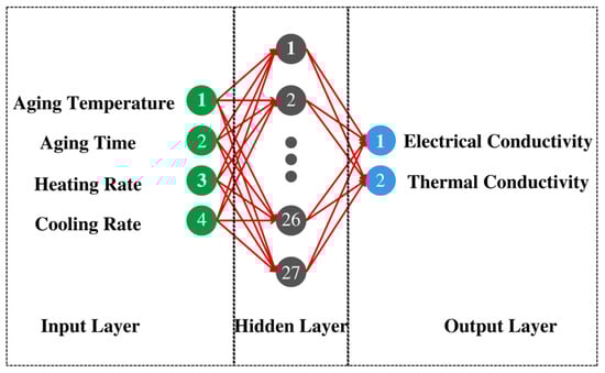
Figure 6. Structure of Back Propagation Artificial Neural Network used in the study.

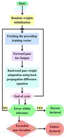
Figure 7. Algorithm for the back-propagation artificial neural network program.

Back-propagation network—algorithm:

Using a flowchart depicted in Figure 7, the algorithm for the back-propagation network software is discussed in the next section.

Step 1: Choosing the number of hidden layers;

Step 2: Choosing the number of neurons for both the input and output layers. The number of neurons in the input layer corresponds to the number of input variables, and the number of neurons in the output layer corresponds to the number of required outputs;

Step 3: Importing the input training pattern;

Step 4: Assigning minimal weight values to the neurons interconnected between the input, hidden, and output layers;

Step 5: Calculating the output values for all neurons in the output and hidden layers using Equation (6)

$$ou{t}_i=f\left(ne{t}_1\right)=f\left({\displaystyle \sum }_{w_{ij}}ou{t}_j+{\theta }_1\right)$$

(6)

where, out ‘i’ = “output of the ith neuron”; out ‘j’ = “output of the jth neuron” and ‘f’ = “sigmoid function” (Equation (7))

$$f\left(ne{t}_1\right)=\frac{1}{1+e^{-net\frac{i}{q}}}$$

(7)

where q is termed as temperature;

Step 6: Establish the performance at the output layer and correlate the results to the required output values.

Establish the inaccuracy of the output neurons,

error = desired output − actual output

Similarly, establish the “root mean square error value” of the output neurons using Equation (8).

$$E_p=\frac{1}{2}\sum {\left(t_{pj}-O_{pj}\right)}^2$$

(8)

where, E_p = “error for the pth presentation vector”, t_pj = “desired value for the jth output neuron” and O_pj = “desired output of the jth output neuron”;

Step 7: Compute the error available at the hidden layer neurons and back-propagate it against the weight values linking the hidden layer neurons and input layer neurons. Back propagate the errors visible at the output values, connecting the hidden layer and output layer neurons using Equations (9)–(11).

$$error {\delta }_{pi}=\left(t_{pi}-O_{pi}\right)O_{pi}\left(1-O_{pi}\right)$$

(9)

For output neurons

$$error {\delta }_p=(t_{pi}-O_{pi})O_{pi}\sum {\delta }_{pi}{W}_{ki}$$

(10)

For hidden neurons

Weight adjustment is made as follows:

$$\Delta W_{ij}\left(n=1\right)=\vartheta \left({\delta }_{pi}{O}_{pi}\right)=\alpha \Delta W_{ij}\left(n\right)$$

(11)

where $\vartheta$ is the learning rate parameter and αis the momentum factor;

Step 8: Continue to Step 3 and calculate through Step 7. After the cycle, compute the root-mean-square error, the standard proportion of error, and the lowest error percentage for the entire pattern. If the inaccuracy is reasonable, go to Step 9; if not, return to Step 3 and repeat Steps 3 through 7;

Step 9: Stop the loop and record the final weight values for the neurons in the output layer and the hidden layer;

Step 10: Evaluate the neural model using training weight values, computing output for testing pattern, and deciding if the deviation from the predicted value is acceptable. If not, attempt back-propagation by altering the number of neurons, training rate parameters, momentum level, and temperature value of the modified network. Typical network performance findings collected during pattern testing are displayed in Table 9.

Table 9. Observations of the output response.

Itinerary	Description
Configuration of the network	4-27-2
Hidden Layer	1
Hidden neurons	27
Applied transfer function	“Logsig (sigmoid)”
Training pattern count	9
Testing pattern count	9
Epoch count	8000
(η) Factor for learning	0.6
(α) Factor of momentum	1

3. Results and Discussions

Electrical and thermal conductivity study following the processing of Ti-6Al-4V-SiC (15 Wt%.) has proven to be the most effective method for determining the physical properties. In this part, therefore, the influence of process input parameters such as aging temperature (°C), aging time (h), heating rate (°C/min), and cooling rate (°C/min) on process output parameters such as electrical and thermal conductivity based on L₉ Orthogonal Array is explored. In addition, the response surface methodology and back propagation artificial neural network technique have been modified to anticipate the optimal process input parameters to optimize electrical and thermal conductivity. Finally, the microstructural investigation of Ti-6Al-4V-SiC (15 Wt%.) under various processing parameters has been discussed.

3.1. Electrical Conductivity

From the experimental results (Figure 8) using Taguchi’s L₉ orthogonal array for electrical conductivity we can observe that the electrical conductivity decreased at 1050 °C and 1250 °C aging temperatures, compared to 1150 °C, which is considered the optimum aging temperature for the formation of ternary carbides of titanium silicon carbide (Ti₃SiC₂). At 1150 °C aging temperature, highly dense Ti₃SiC₂ structures are formed due to the higher diffusion rates compared to 1250 °C aging temperature where a less electrically conductive TiSi₂ phase is formed. Further aging time of four hours is the optimum aging time allowing for the complete transformation of Ti₃SiC₂. Heating and cooling rates during processing did not show much difference in electrical conductivity compared to aging temperature and aging time. However, with an 1150 °C aging temperature and four hours of aging time with a 25 °C/min heating rate and a 5 °C/min cooling rate, the lowest porosity was observed (Figure 8) However, the electrical conductivity of a material is affected by the percentage of porosity due to the hindered flow of free electrons [34]. Therefore, the highest electrical conductivity of 4,260,000 Ω⁻¹ m⁻¹ has been observed with the samples with the lowest percentage of porosity.

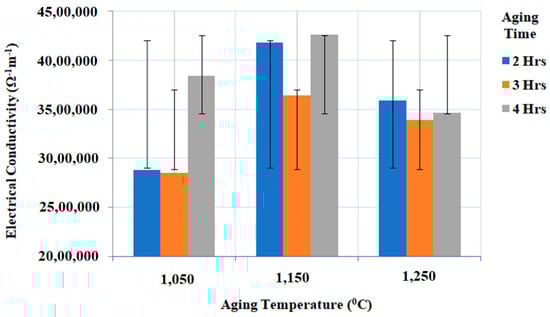
Figure 8. Experimental results of electrical conductivity (Ω⁻¹ m⁻¹) under different aging temperatures (°C) and aging times (h) with the constant heating rate (°C/min), and cooling rate (°C/min).

Figure 9 presents the electrical conductivity versus temperature for Ti-6Al-4V-SiC (15 Wt.%) specimen processed at aging temperature (1150 °C), aging time (4 h), heating rate (25 °C/min) and cooling rate (5 °C/min) while cooling from (a) 360–13 °C and (b) heating from 13–360 °C. From the graphical representation (Figure 9b) we can observe that, with temperature increases, the electrical conductivity of the Ti-6Al-4V-SiC (15 Wt.%) composite decreases.

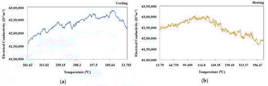
Figure 9. Electrical conductivity versus temperature for Ti-6Al-4V-SiC (15 Wt.%) specimen processed at aging temperature (1150 °C), aging time (four hours), heating rate (25 °C/min), and cooling rate (5 °C/min) while cooling from 360–13 °C.

From the main effects plot (Figure 10) for electrical conductivity, it can be seen that the selection of aging temperature (1150 °C), aging time (four hours), heating rate (25 °C/min), and cooling rate (5 °C/min) have resulted as the optimal combination for obtaining the highest electrical conductivity value during the processing of Ti-6Al-4V-SiC (15 Wt.%) composites.

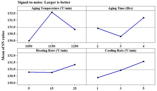
Figure 10. Main effects plot for electrical conductivity (Ω⁻¹ m⁻¹).

Further, from Figure 11, using XRD, the presence of Ti₃SiC₂ phase under aging temperature (1150 °C), aging time (four hours), heating rate (25 °C/min), and cooling rate (5 °C/min) resulted in increased thermal and electrical conductivity [35].

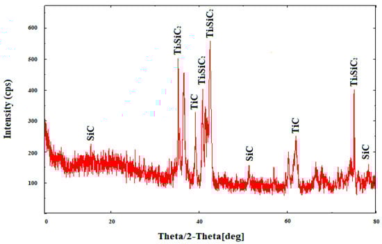
Figure 11. XRD Peaks of Ti-6Al-4V-SiC(15 Wt.%) processed under aging temperature (1150 °C), aging time (four hours), heating rate (5 °C/min), and cooling rate (5 °C/min).

The second order model (Equation (12)) which has been generated using response surface methodology for electrical conductivity can be expressed as a “function of processing parameters” such as aging temperature (°C), aging time (h), heating rate (°C/min) and cooling rate (°C/min) as shown in Equation (6) from the coefficients of regression estimated (Table 10).

Electrical Conductivity (Ω⁻¹ m⁻¹) = 3,825,280 + 134,444A + 153,333B + 16,667C + 321,667D − 774,773A² + 305,227B² + 75,227C² + 80,227D² + 26,250AB − 18,750AC + 53,750AD − 18,750BC + 13,750BD − 18,750CD

(12)

Table 10. Estimated Regression Coefficients for Electrical Conductivity (Ω⁻¹ m⁻¹).

Term	Coef	SE Coef	T	P
Constant	3,825,280	22,155	172.660	0.000
A	134,444	17,603	7.637	0.000
B	153,333	17,603	8.710	0.000
C	16,667	17,603	0.947	0.358
D	321,667	17,603	18.273	0.000
A*A	−774,773	46,361	−16.712	0.000
B*B	305,227	46,361	6.584	0.000
C*C	75,227	46,361	1.623	0.124
D*D	80,227	46,361	1.730	0.103
A*B	26,250	18,671	1.406	0.179
A*C	−18,750	18,671	−1.004	0.330
A*D	53,750	18,671	2.879	0.011
B*C	−18,750	18,671	−1.004	0.330
B*D	13,750	18,671	0.736	0.472
C*D	−18,750	18,671	−1.004	0.330

Aging Temperature (°C)—A; Aging Time (h)—B; Heating Rate (°C/min)—C; Cooling Rate (°C/min)—D.

The ANOVA result for the response function (electrical conductivity) has been provided in Table 11. This analysis was conducted using a “5% level of significance, or a 95% level of confidence”. It can be seen that the estimated F value is more than the F-table value (F_0.05,14,16 = 59.57), indicating that the generated second-order response function is fairly sufficient.

Table 11. Analysis of variance for electrical conductivity.

Source	DF	Seq SS	Adj SS	Adj MS	F	P
Regression	14	4.65159 × 1012	4.65159 × 1012	3.32257 × 1011	59.57	0.000
Residual Error	16	89,244,311,111	89,244,311,111	5,577,769,444		0.000
Total	30	4.74084 × 1012

Contour and surface plots for electrical conductivity (Ω⁻¹ m⁻¹) presented in Figure 12a, clearly indicate that maximum electrical conductivity (<44,766,021 Ω⁻¹ m⁻¹) has been achieved with aging temperature (1150 °C), aging time (four hours), heating rate (25 °C/min), and cooling rate (5 °C/min).

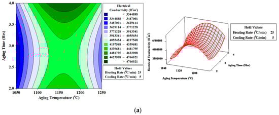
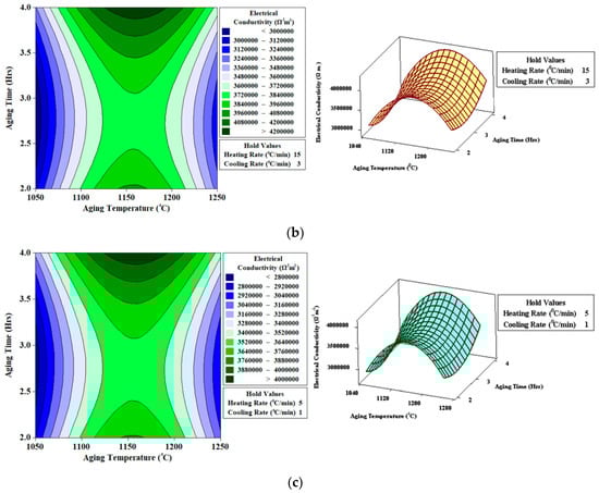
Figure 12. Contour and surface plots for electrical conductivity (Ω⁻¹ m⁻¹) (a) Heating Rate (25 °C/min); Cooling Rate (5 °C/min) (b) Heating Rate (15 °C/min); Cooling Rate (3 °C/min) (c) Heating Rate (5 °C/min); Cooling Rate (1 °C/min).

3.2. Thermal Conductivity

From experimental results using an L₉ orthogonal array, in Figure 13 it is observed that the thermal conductivity decreased at 1050 °C and 1250 °C aging temperature, compared to 1150 °C. Aging temperature and aging time determine the density of the Ti-6Al-4V-SiC composites and facilitate the proper formation of Ti₃SiC₂. At 1150 °C aging temperature and four hours of aging time, minimum porosity corresponding to maximum thermal conductivity (36.15 W/m·K) has been observed. Further, with a heating rate of 25 °C/min and a rapid cooling rate of 5 °C/min, delocalized electrons were formed which improved the thermal conductivity of the Ti-6Al-4V-SiC (15 Wt.%) composite. Furthermore, strong localized bonds of Ti-C and Ti-Si were formed at 1150 °C compared to the 1250 °C aging temperature, improving the thermal conductivity of the Ti-6Al-4V-SiC (15 Wt.%) composite specimen.

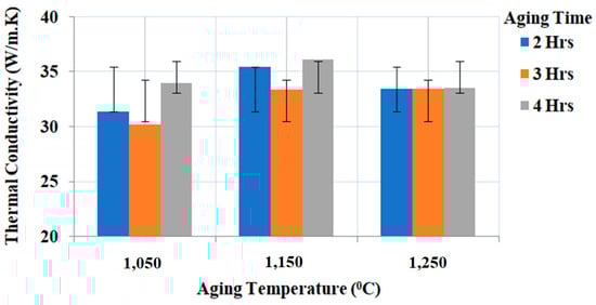
Figure 13. Experimental results plot for thermal conductivity.

Figure 14 presents the thermal conductivity versus temperature for Ti-6Al-4V-SiC (15 Wt.%) specimen processed at aging temperature (1150 °C), aging time (four hours), heating rate (25 °C/min), and cooling rate (5 °C/min), while heating from 30–1000 °C.

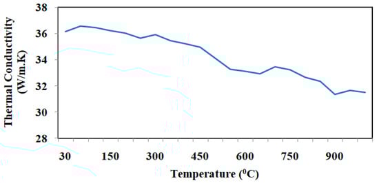
Figure 14. Thermal conductivity versus temperature plot of Ti-6Al-4V-SiC(15 Wt.%) processed under aging temperature (1150 °C), aging time (four hours), heating rate (5 °C/min), and cooling rate (5 °C/min).

From the main effects plot (Figure 15) for thermal conductivity, it can be observed that the combination of aging temperature (1150 °C), aging time (three hours), heating rate (25 °C/min), and cooling rate (5 °C/min) has resulted in the higher thermal conductivity value during the processing of Ti-6Al-4V-SiC(15 Wt.%) composites.

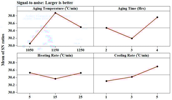
Figure 15. Main effects plot for thermal conductivity.

The second-order model representing the thermal conductivity can be expressed as a “function of processing parameters”(Equation (13)) such as aging temperature (°C), aging time (hours), heating rate (°C/min), and cooling rate (°C/min) as shown in Equation (8) using the estimated regression coefficients (Table 12).

Thermal Conductivity = 33.8420 + 0.4628A + 0.5256B + 0.0567C + 0.8506D − 2.559A² + 1.356B² + 0.156C² + 0.521D² + 0.2075AB − 0.0637AC + 0.0875AD − 0.0637BC − 0.0225BD − 0.0638CD

(13)

Table 12. Estimated regression coefficients for thermal conductivity (W/m·K).

Term	Coef	SE Coef	T	P
Constant	33.8480	0.09255	365.719	0.000
A	0.4628	0.07354	6.293	0.000
B	0.5256	0.07354	7.147	0.000
C	0.0567	0.07354	0.771	0.452
D	0.8506	0.07354	11.566	0.000
A*A	−2.5590	0.19367	−13.213	0.000
B*B	1.3560	0.19367	7.002	0.000
C*C	0.1560	0.19367	0.805	0.432
D*D	0.5210	0.19367	2.690	0.016
A*B	0.2075	0.07800	2.660	0.017
A*C	−0.0637	0.07800	−0.817	0.426
A*D	0.0875	0.07800	1.122	0.278
B*C	−0.0637	0.07800	−0.817	0.426
B*D	−0.0225	0.07800	−0.288	0.777
C*D	−0.0638	0.07800	−0.817	0.426

Aging Temperature (°C)—A; Aging Time (h)—B; Heating Rate (°C/min)—C; Cooling Rate (°C/min)—D.

Table 13 presents the ANOVA result for the response function thermal conductivity. This analysis was conducted using a “5% level of significance, or a 95% level of confidence”. Analysis from Table 13 demonstrates that the estimated F value is bigger than the F-table value (F_{0.05,14, 14} = 30.69), indicating that the generated second-order response function is fairly sufficient.

Table 13. Analysis of variance for thermal conductivity (W/m·K).

Source	DF	Seq SS	Adj SS	Adj MS	F	P
Regression	14	41.822	41.8222	2.98730	30.69	0.000
Residual Error	16	1.5574	1.5574	0.09734
Total	30	43.3796

Contour and surface plots for electrical conductivity (Ω⁻¹ m⁻¹) presented in Figure 16a, clearly show that maximum thermal conductivity (36.7214–37.2107 W/m·K) can be achieved with aging temperature (1150 °C), aging time (four hours), heating rate (25 °C/min), and cooling rate (5 °C/min).

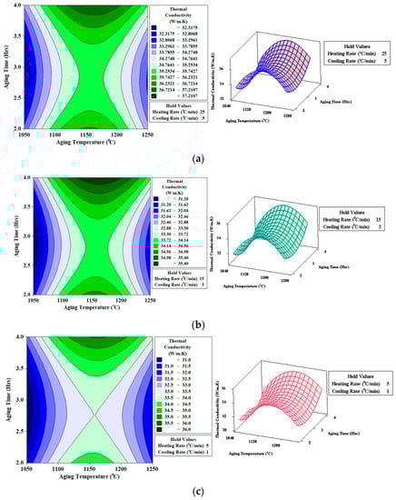
Figure 16. Contour and surface plots for thermal conductivity (W/m·K) (a) Heating Rate (25 °C/min); Cooling Rate (5 °C/min) (b) Heating Rate (15 °C/min); Cooling Rate (3 °C/min) (c) Heating Rate (5 °C/min); Cooling Rate (1 °C/min).

3.3. Validation of Electrical and Thermal Conductivity

For the validation of electrical and thermal conductivity values obtained from the L₉ orthogonal array with second-order response surface model and BPANN model for nine sets of trials, it was noted that the value estimated is very accurate for all the conducted tests with a minimal error of 0.72% and 0.86% with RSM and 0.39% and 0.48% with BPANN estimated values for electrical conductivity and thermal conductivity, respectively. However, BPANN has been trained with 27 nodes in the hidden layer. The performance of BPANN while testing all the patterns (training and testing) was found to be excellent with a minimal error (1.47%). The BPANN model has been rigorously tested utilizing the training data and corresponding graphs that have been plotted using predicted and tested values (Figure 17) (Table 14). The results indicate that the BPANN model has been successfully applied with an error percentage of 0.39% for electrical conductivity (Ω⁻¹ m⁻¹)and 0.48% for thermal conductivity (W/m·K), respectively. The calculated error is considered reasonable and shows that the BPANN model has been successfully applied for predicting the electrical and thermal conductivity of vacuum-sintered Ti-6Al-4V-SiC (15 Wt.%).

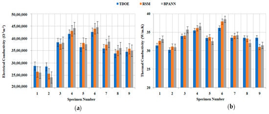
Figure 17. Experimental versus RSM versus BPANN prediction values of (a) electrical conductivity and (b) thermal conductivity.

Table 14. Electrical conductivity and thermal conductivity of Ti-6Al-4V-SiC(15 Wt.%) specimen processed under various processing conditions.

Trial No.	Electrical Conductivity (Ω−1 m−1)			Error (%)		Thermal Conductivity (W/m·K)			Error (%)
	TDOE	RSM	BPANN	RSM	BPANN	TDOE	RSM	BPANN	RSM	BPANN
1	2,880,000	2,641,592	2,611,491	9.025	1.152	31.41	32.59844	33.1425	3.645	1.641
2	2,850,000	2,567,891	2,415,789	10.98	6.296	30.22	31.11954	30.95	2.89	0.547
3	3,840,000	3,769,585	3,825,495	1.867	1.461	33.95	34.05957	35.6830	0.321	4.549
4	4,180,000	4,305,898	4,413,895	2.923	2.446	35.46	36.07785	36.5815	1.712	1.376
5	3,640,000	3,812,258	3,764,822	4.518	1.259	33.41	33.64925	32.5512	0.711	3.373
6	4,260,000	4,393,699	4,452,174	3.042	1.313	36.15	37.88915	38.4951	4.59	1.574
7	3,590,000	3,745,102	3,862,733	4.141	3.045	33.46	33.99454	34.1920	1.572	0.577
8	3,390,000	3,508,955	3,605,897	3.390	2.688	33.49	33.24958	32.0552	0.723	3.726
9	3,460,000	3,577,488	3,498,621	3.284	2.254	33.51	31.01259	31.4586	8.052	1.417

3.4. Microstructural Analysis

Figure 18a–i presents the microscopic images of vacuum sintered Ti-6Al-4V-SiC(15 Wt.%) composite based on L₉ orthogonal array using an Olympus IMS BX53M system optical microscope. Different grades of porosity characterized as black spots can be observed depending on the process input parameters of the vacuum sintering process i.e., aging temperature (°C), aging time (hours), heating rate (°C/min), and Cooling Rate (°C/min). The lowest porosity corresponding to the highest electrical and thermal conductivity has been observed with the sample produced at an aging temperature (1150 °C), aging time (four hours), heating rate (25 °C/min), and cooling rate (5 °C/min).

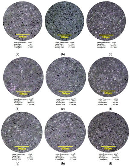
Figure 18. Metallographic images of Ti-6Al-4V-SiC(15 Wt.%) processed under various conditions.

Scanning electron microscopy with elemental mapping using X-rays was used to analyze the microstructure of a Ti-6Al-4V-SiC (15 Wt.%) specimen processed under aging temperature (1150 °C), aging time (four hours), heating rate (25 °C/min), and cooling rate (5 °C/min). The microstructure (Figure 19) grains of Ti₃SiC₂ can be identified along with void spaces and un-transformed SiC particulates embedded in the Ti-6Al-4V matrix alloy. From the elemental mapping (Figure 20) of the Ti-6Al-4V-SiC(15 Wt.%) specimen, the distribution of elements (titanium, silicon, and, carbon) can be seen. The homogenous distribution of carbon indicates the isotropic presence of ternary carbide phases of titanium, ascertaining the formation of Ti₃SiC₂.

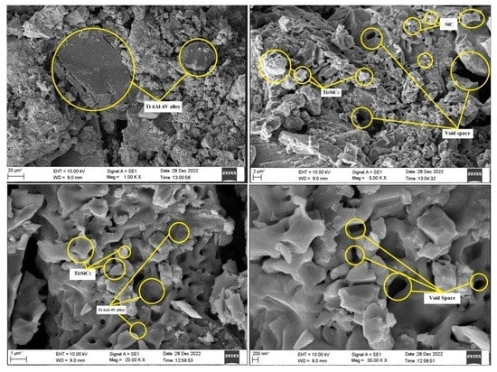
Figure 19. Scanning Electron Microscope images of Ti-6Al-4V-SiC(15 Wt.%) processed under aging temperature (1150 °C), aging time (four hours), heating rate (25 °C/min), and cooling rate (5 °C/min).

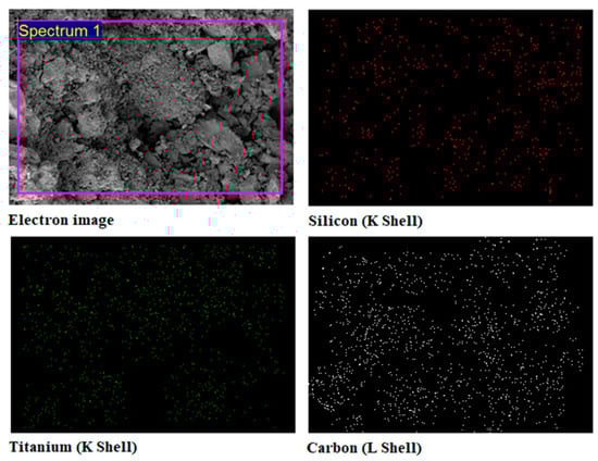
Figure 20. Elemental Mapping of Ti-6Al-4V-SiC(15 Wt.%) composite processed under aging temperature (1150 °C), aging time (four hours), heating rate (25 °C/min), and cooling rate (5 °C/min) from electron dispersive X-ray analysis.

4. Conclusions

The electrical conductivity and thermal conductivity of Ti-6Al-4V-SiCp composites processed under various processing conditions have been studied utilizing Taguchi’s L₉ orthogonal array, response surface methodology (RSM), and back propagation artificial neural network (BPANN). Based on the results, the following conclusions are drawn:

• Using Taguchi’s L₉ Orthogonal Array it has been observed that, aging temperature (1150 °C), aging time (four hours), heating rate (25 °C/min), and cooling rate (5 °C/min) result as optimum input parameters for achieving the highest electrical conductivity values during the processing of Ti-6Al-4V-SiCp composites. Furthermore, for maximum thermal conductivity values during the processing of Ti-6Al-4V-SiCp composites, aging temperature (1150 °C), aging time (four hours), heating rate (5 °C/min), and cooling rate (5 °C/min) are preferred;
• A second-order response surface model generated can be effectively used for predicting the electrical conductivity and thermal conductivity during the processing of Ti-6Al-4V-SiCp composites with an accuracy of 99.28% (electrical conductivity) and 99.14% (thermal conductivity);
• By comparing the experimental results along with the results of the mathematical model and BPANN model results for nine trials, it was observed that the estimated value is accurate for all tests with an error of 0.39% (electrical conductivity) and 0.48% (thermal conductivity);
• Furthermore, from X-ray diffraction studies and microstructural analysis, it has been observed that, aging at 1150 °C for four hours resulted in the formation of a ternary carbide phase of titanium silicon carbide (Ti₃SiC₂) which resulted in maximum electrical conductivity (4,260,000 Ω⁻¹ m⁻¹) and thermal conductivity (36.42 W/m·K) of Ti-6Al-4V-SiC (15 Wt.%) composite specimen.

References

- Barsoum, M.W. The MN+1AXN phases: A new class of solids: Thermodynamically stable nanolaminates. Prog. Solid St. Chem. 2000, 28, 201. [Google Scholar] [CrossRef]
- Barsoum, M.W.; El-Raghy, T. Synthesis and Characterization of a Remarkable Ceramic: Ti3SiC2. J. Am. Ceram. Soc. 1996, 79, 1953–1956. [Google Scholar] [CrossRef]
- El-Raghy, T.; Barsoum, M.W. Processing and Mechanical Properties of Ti3SiC2: I, Reaction path and microstructure evolution. J. Am. Ceram. Soc. 1999, 82, 2849–2854. [Google Scholar] [CrossRef]
- Goto, T.; Hirai, T. Chemically vapour deposited Ti3SiC2. Mater. Res. Bull. 1987, 22, 1195. [Google Scholar] [CrossRef]
- Jeitschko, W.; Nowotny, H. Synthesis of Ti3SiC2–Bi-carbide based ceramic electro-thermal explosion. Mon. Chem. 1967, 98, 329. [Google Scholar] [CrossRef]
- Li, J.T.; Miyamoto, Y. Fabrication of Monolithic Ti3SiC2 ceramic through reactive sintering of Ti/SiC2TiC. J. Mater. Synth. Proc. 1999, 7, 91. [Google Scholar] [CrossRef]
- Sun, Z.M.; Hashimoto, H. Synthesis and Characterization of a Metallic Ceramic Material—Ti3SiC2. Metall. Mater. Trans. 2002, 33, 3321–3328. [Google Scholar]
- Pampuch, R.; Lis, J.; Stobierski, L.; Tymkiewicz, M. Synthesis of Sinterable beta-SiC powders by a Solid Combustion method. J. Eur. Ceram. Soc. 1989, 5, 283. [Google Scholar] [CrossRef]
- Gonzalez, C.; Llroca, J. Micro-mechanical modelling of deformation and failure in Ti-6Al-4V/SiC composites. Acta Mater. 2001, 49, 3505–3519. [Google Scholar] [CrossRef]
- Misra, S.; Hussain, M.; Gupta, A.; Kumar, V.; Kumar, S.; Das, A.K. Fabrication and characteristic evaluation of direct metal laser sintered SiC particulate reinforced Ti6Al4V metal matrix composites. J. Laser Appl. 2019, 31, 012005. [Google Scholar] [CrossRef]
- Sivakumar, G.; Ananthi, V.; Ramanathan, S. Production and mechanical properties of nano SiC particle reinforcedTi-6Al-4V matrix composite. Trans. Nonferrous Met. Soc. China 2017, 27, 82–90. [Google Scholar] [CrossRef]
- Amiri, S.H.; Kakroudi, M.G.; Rabizadeh, T.; Asl, M.S. Characterization of hot-pressed Ti3SiC2-SiC composites. Int. J. Refract. Met. Hard Mater. 2020, 90, 105232. [Google Scholar] [CrossRef]
- Sun, Z.M.; Wang, Q.; Hashimoto, H.; Tada, S.; Abe, T. Synthesis and characterization of a metallic ceramic material—Ti3SiC2. Intermetallics 2003, 11, 63. [Google Scholar] [CrossRef]
- Prajapati, P.K.; Chaira, D. Fabrication and Characterization of Cu-B4C Metal Matrix Composite by Powder Metallurgy: Effect of B4C on Microstructure, Mechanical properties and Electrical Conductivity. Trans. Indian Inst. Met. 2019, 72, 673–684. [Google Scholar] [CrossRef]
- Islak, B.Y.; Ayas, E. Evaluation of properties of Spark plasma sintered Ti3SiC2 and Ti3SiC2/SiC composites. Ceram. Int. 2019, 45, 12297–12306. [Google Scholar] [CrossRef]
- Esmati, M.; Sharifi, H.; Raesi, M.; Atrian, A.; Rajaee, A. Investigation into thermal expansion coefficient, thermal conductivity and thermal stability of Al-Graphite composite prepared by powder metallurgy. J. Alloys Compd. 2018, 773, 503–510. [Google Scholar] [CrossRef]
- Sergi, A.; Raja Khan, H.U.; Irukuvarghula, S.; Meisnar, M.; Makaya, A.; Attallah, M.M. Development of Ni-base metal matrix composites by powder metallurgy hot isostatic pressing for space applications. Adv. Powder Technol. 2022, 3, 103411. [Google Scholar] [CrossRef]
- Kumar, M.; Gupta, R.K.; Pandey, A. Study on properties and selection of metal matrix and reinforcement material for composites. Int. J. Interact. Des. Manuf. 2022, 1–12. [Google Scholar] [CrossRef]
- Hasselman, D.P.H.; Donaldson, K.Y.; Geiger, A.L. Effect of Reinforcement Particle size on the thermal conductivity of a particulate silicon carbide reinforced aluminium matrix composite. J. Am. Ceram. Soc. 1992, 75, 3137–3140. [Google Scholar] [CrossRef]
- Hegde, A.L.; Shetty, R.; Chiniwar, D.; Naik, N.; Nayak, R.; Nayak, M. Optimization and Prediction of Mechanical Characteristics on Vacuum Sintered Ti-6Al-4V-SiCp Composites using Taguchi’s Design of Experiments, Response Surface Methodology and Random Forest Regression. J. Compos. Sci. 2022, 6, 339. [Google Scholar] [CrossRef]
- Shetty, R.; Hegde, A. Taguchi based fuzzy logic model for optimization and prediction of surface roughness during AWJM of DRCUFP composites. Manuf. Rev. 2022, 9, 2. [Google Scholar] [CrossRef]
- Shetty, R.; Pai, R.B.; Rao, S.S.; Nayak, R. Taguchi’s technique in machining of metal matrix composites. J. Braz. Soc. Mech. Sci. Eng. 2009, 31. [Google Scholar] [CrossRef]
- Shetty, R.; Pai, R.; Rao, S.S. Experimental Studies on Turning of Discontinuosuly Reinforced Aluminium Composites under Dry, Oil Water Emulsion and Steam Lubricated conditions using Taguchi’s technique. Gazi Univ. J. Sci. 2009, 22, 21–32. [Google Scholar]
- Jayashree, P.K.; Sharma, S.S.; Shetty, R.; Mahato, A.; Gowrishankar, M.C. Optimization of TIG welding parameters for 6061 Al alloy using Taguchi’s design of experiments. Mater. Today Proc. 2018, 5, 23648–23655. [Google Scholar] [CrossRef]
- Balakrishna, M.; Radhika, P.B.; Vivek, S. Statistical Evaluation of Mechanical Properties of Green Cement Concretes—Taguchi Integrated Supervized Learning Approach. Eng. Sci. 2022, 18, 148–158. [Google Scholar]
- Kamath, G.; Subramaniam, K.; Devesh, S. Multi-response optimization of milling process parameters for Aluminium–Titanium Diboride Metal Matrix Composite Machining using Taguchi-Data Envelopment Analysis Ranking approach. Eng. Sci. 2022, 18, 271–277. [Google Scholar] [CrossRef]
- Hiremath, A.; Thipperudrappa, S.; Bhat, R. Surface Morphology Analysis using Atomic Force Microscopy and Statistical Method for Glass Fiber Reinforced Epoxy-Zinc Oxide nanocomposites. Eng. Sci. 2022, 18, 308–319. [Google Scholar] [CrossRef]
- Chougale, A.; Shelke, H.D.; Prasad, B.; Jadkar, S.R.; Naik, N.; Pathan, H.M.; Shindhe, D.R. Simulation of p-CdTe and n-TiO2 Heterojunction solar cell efficiency. J. Comput. Mech. Manag. 2023, 2, 1. [Google Scholar] [CrossRef]
- Natesh, C.P.; Shashidhara, Y.M.; Amarendra, H.J.; Shetty, R.; Harisha, S.R.; Shenoy, P.V.; Nayak, M.; Hegde, A.; Shetty, D.; Umesh, U. Tribological and Morphological Study of AISI 316L Stainless Steel during Turning under Different Lubrication conditions. Lubricants 2023, 11, 52. [Google Scholar] [CrossRef]
- Shetty, R.; Pai, R.; Barboza, A.B.; Shetty, Y. Statistical and surface metallurgical study during electric discharge machining of Ti-6Al-4V. ARPN J. Eng. Appl. Sci. 2018, 13, 3594–3600. [Google Scholar]
- Shetty, R.; Barboza, A.B.V.; Kini, L.G. Empirical study on stress distribution zone during machining of DRACs using finite element analysis, Taguchi’s design of experiments and response surface methodology. ARPN J. Eng. Appl. Sci. 2019, 14, 2576–2582. [Google Scholar]
- Karthik, S.R.; Londe, N.V.; Shetty, R.; Nayak, R.; Hegde, A. Optimization and prediction of hardness, wear and surface roughness on age hardened stellite 6 alloys. Manuf. Rev. 2022, 9, 10. [Google Scholar] [CrossRef]
- Shetty, R.; Gurupur, P.R.; Hindi, J.; Hegde, A.; Naik, N.; Ali, M.S.S.; Patil, I.S.; Nayak, M. Processing, Mechanical Characterization and Electric discharge machining of Stir cast and Spray forming-based Al-Si alloy reinforced with ZrO2 particulate composites. J. Compos. Sci. 2022, 6, 323. [Google Scholar] [CrossRef]
- Sun, T.M.; Dong, L.M.; Wang, C.; Liang, T.X. Effect of porosity on the electrical resistivity of carbon materials. New Carbon Mater. 2013, 28, 349–354. [Google Scholar] [CrossRef]
- Jiang, M.; Chengguo, L.; Gao, S.; Kate, S.H. Reactively synthesized porous Ti3SiC2 compound and its mechanical properties with different apertures. Crystals 2020, 10, 82. [Google Scholar] [CrossRef]
Disclaimer/Publisher’s Note: The statements, opinions and data contained in all publications are solely those of the individual author(s) and contributor(s) and not of MDPI and/or the editor(s). MDPI and/or the editor(s) disclaim responsibility for any injury to people or property resulting from any ideas, methods, instructions or products referred to in the content. |
© 2023 by the authors. Licensee MDPI, Basel, Switzerland. This article is an open access article distributed under the terms and conditions of the Creative Commons Attribution (CC BY) license (https://creativecommons.org/licenses/by/4.0/).