Evaluation of a Baseline Controller for Autonomous “Figure-8” Flights of a Morphing Geometry Quadcopter: Flight Performance

1
Department of Aerospace and Mechanical Engineering, Parks College of Engineering, Aviation and Technology, Saint Louis University, St. Louis, MO 63103, USA
2
Aerospace Engineering Parks College of Engineering, Aviation and Technology, Saint Louis University, St. Louis, MO 63103, USA
*
Author to whom correspondence should be addressed.
†
These authors contributed equally to this work.
Drones 2019, 3(3), 70; https://doi.org/10.3390/drones3030070
Submission received: 5 July 2019
/
Revised: 28 August 2019
/
Accepted: 28 August 2019
/
Published: 31 August 2019
Abstract
:This article describes the design, fabrication, and flight test evaluation of a morphing geometry quadcopter capable of changing its intersection angle in-flight. The experiments were conducted at the Aircraft Computational and Resource Aware Fault Tolerance (AirCRAFT) Lab, Parks College of Engineering, Aviation and Technology at Saint Louis University, St. Louis, MO. The flight test matrix included flights in a “Figure-8” trajectory in two different morphing configurations (21° and 27°), as well as the nominal geometry configuration, two different flight velocities (1.5 m/s and 2.5 m/s), two different number of waypoints, and in three planes—horizontal, inclined, and double inclined. All the experiments were conducted using standard, off-the-shelf flight controller (Pixhawk) and autopilot firmware. Simulations of the morphed geometry indicate a reduction in pitch damping (42% for 21° morphing and 57.3% for 27° morphing) and roll damping (63.5% for 21° morphing and 65% for 27° morphing). Flight tests also demonstrated that the dynamic stability in roll and pitch dynamics were reduced, but the quadcopter was still stable under morphed geometry conditions. Morphed geometry also has an effect on the flight performance—with a higher number of waypoints (30) and higher velocity (2.5 m/s), the roll dynamics performed better as compared to the lower waypoints and lower velocity condition. The yaw dynamics remained consistent through all the flight conditions, and were not significantly affected by asymmetrical morphing of the quadcopter geometry. We also determined that higher waypoint and flight velocity conditions led to a small performance improvement in tracking the desired trajectory as well.
1. Introduction
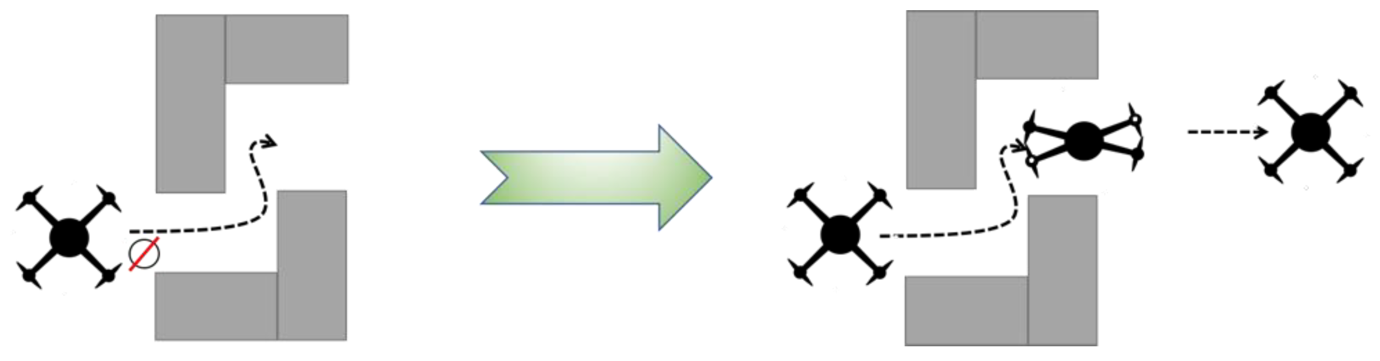
Multi-copters, including commonly used platforms such as quadcopters, hexacopters, octocopters, or their variants, are popular as base aerial platforms for many civilian applications, including remote sensing [1,2,3], aerial imaging [4,5], firefighting [6,7], environmental measurement [8,9,10], law enforcement [11,12,13], disaster relief and emergency management [14,15,16,17,18], situational awareness [19] infrastructure surveys [20], and several other military and commercial applications. Quadcopters can be considered to be representative of this general class of aircraft, and can be maneuvered by varying the power of the four motors symmetrically or asymmetrically in order to achieve translational and rotational flight. While these platforms are well suited to execute a wide variety of aerial tasks, their physical geometry plays a significant role in defining the applicability of a particular platform for a particular task; for instance, if the Unmanned Aerial System (UAS) is required to carry a suite of sensors, such as large cameras, LIDAR, or hyperspectral imagers, it then follows naturally that the UAS platform should be large enough to carry all the sensors, and be capable of executing the mission according to requirements. On the other hand, if the quadcopter is physically small (to fly through confined spaces), it then restricts the amount of payload it can carry and its flight endurance. This poses a problem in cases where the UAS platform is required to carry a large payload, but still be able to navigate through confined spaces. A compromise option that would allow the quadcopter to carry a higher payload, while remaining capable of navigating through confined spaces, would be a platform that could change or morph from one geometry to another geometry, reducing its footprint in the process. Such a scenario is illustrated in Figure 1.
In this paper, we present the results from flight test experiments of an asymmetrical morphing geometry quadcopter [21], flying a “Figure-8” flight path under different conditions, conducted at the Aircraft Computational and Resource Aware Fault Tolerance (AirCRAFT) laboratory [22], at Saint Louis University, St. Louis, MO. This quadcopter can temporarily change its physical structure by shrinking its lateral dimension to switch between a normal “X” style quadcopter into a slimmer “X” style quadcopter, with a reduced footprint.
Over the last few years there has been increasing interest in the development of multi-rotor UAS platforms with the ability to change their geometry in order to address similar problems. In a recent effort, the design of a morphing geometry quadcopter was explored, where the geometry of the quadcopter changes for short periods of time as and when traversing through a narrow opening in controlled conditions [23]. In another application [24], a quadcopter was designed to actively change its attitude to a relatively high value and fly through a narrow gap or channel, while maintaining a high translation velocity. In this case, when the quadcopter was highly inclined, the thrust generated a large lateral force and an appreciable increase in its lateral velocity. In order to avoid that case, the quadcopter must fly through the narrow gap with high initial velocity in a short time in order to avoid large lateral and vertical displacement. Another experimental quadcopter was designed with active morphing [25]. In this effort, a custom quadcopter was created with ability to morph by mechanically changing its arms’ length and angle. The authors also investigated LQR control on the full model with partial simplification and linearization, and developed nonlinear numeric optimal control approach; but the quadcopter’s flight with morphing was only tested in simulation. Other efforts have taken a different approach to the concept of morphing geometry, including the design of multirotor platforms with multilink geometries, to serve different goals [26,27]. In [28], a X-style quadcopter was experimentally tested with a crash resilient structure (two of the arms could be detached using magnets). In this effort, a custom developed MRAC flight control algorithm was implemented to accommodate for the uncertainties resulting from morphing geometry. In [29], the authors explore the morphing by pivoting individual arms, thus generating what they term as “H”, “O” and “T” morphologies and evaluated the performance of the quadcopter in both hover conditions and while executing circular trajectories. As with most of the other approaches, a customized Linear Quadratic Regulator (LQR) controller was implemented to maintain the stability and performance of the quadcopter in its morphed configurations.
Our effort is distinct in the fact that we are evaluating the effectiveness of readily available flight control algorithms (PID-based and without modifications)—this is typically included as a part of open source firmware (Ardupilot 3.4.1, in our case [30]) on COTS hardware (Pixhawk [31])—through flight tests in real world conditions, for longer durations as compared to other efforts. Additionally, the experiments flights featured longer flight durations under morphed geometry (approximately 15s on average over all the ~350 flights) and is appreciably different from the experiments described in references [24,30,32]. Furthermore, the flights were performed at different velocities, with a varying number of waypoints, and outdoors—this bringing with it the requirement of the flight controller to address real world disturbances, such as wind gusts.
This article is organized as follows. Section 2 describes the methods and materials used to fabricate the quadcopter and the onboard avionics. Section 3 describes the modeling of the moments of inertia of the quadcopter in its morphed geometry state, and Section 4 describes the simulation and flight test experiments, the results of the tests, as well as observations and conclusions.
2. Materials and Methods
The quadcopter UAS used in this effort was designed and fabricated in-house in the Aircraft Computational and Resource Aware Fault Tolerance (AirCRAFT) Laboratory, at Parks College of Engineering, Saint Louis University. Further details on the design and fabrication of this UAS are given in the following sections.
2.1. Design and Fabrication of the Morphing Geometry Quadcopter
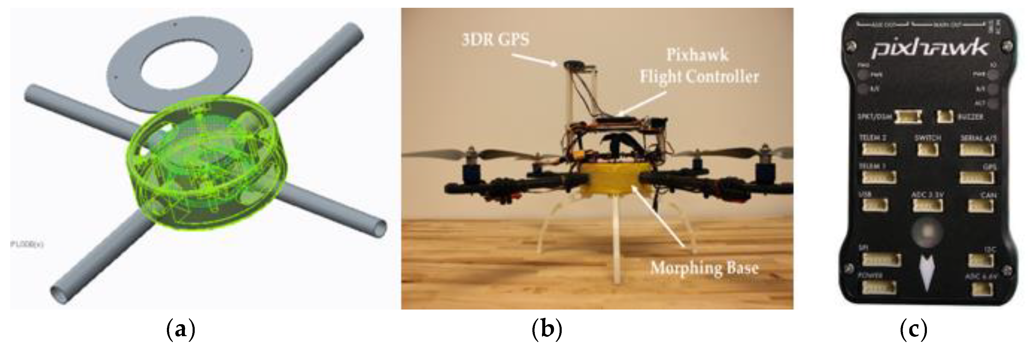
The quadcopter was configured to be an “X-style” platform, with the forward direction of the UAS and the flight controller aligned in between the arms. The central hub of this platform was designed to serve as the morphing base; it is driven by a digital servo mounted on the bottom section of the hub and with its drive shaft aligned with the central axis of rotation of the hub for achieving geometry morphing. A wireframe drawing of the morphing quadcopter assembly is shown in Figure 2a and the flight ready quadcopter is shown in Figure 2b.
2.1.1. Flight Controller
The morphing quadcopter features the widely available Pixhawk (Figure 2c) as the quadcopter’s flight controller; the off the shelf controller includes a three-axis inertial measurement unit (IMU), three-axis gyroscopes, magnetometer, barometer, and redundant interfaces for external sensors and devices. This is augmented with a 3DR GPS module for positioning and to facilitate waypoint navigation. Salient specifications of the Pixhawk controller are listed in Table 1. Additional details can be found in [32].
2.1.2. Propulsion System
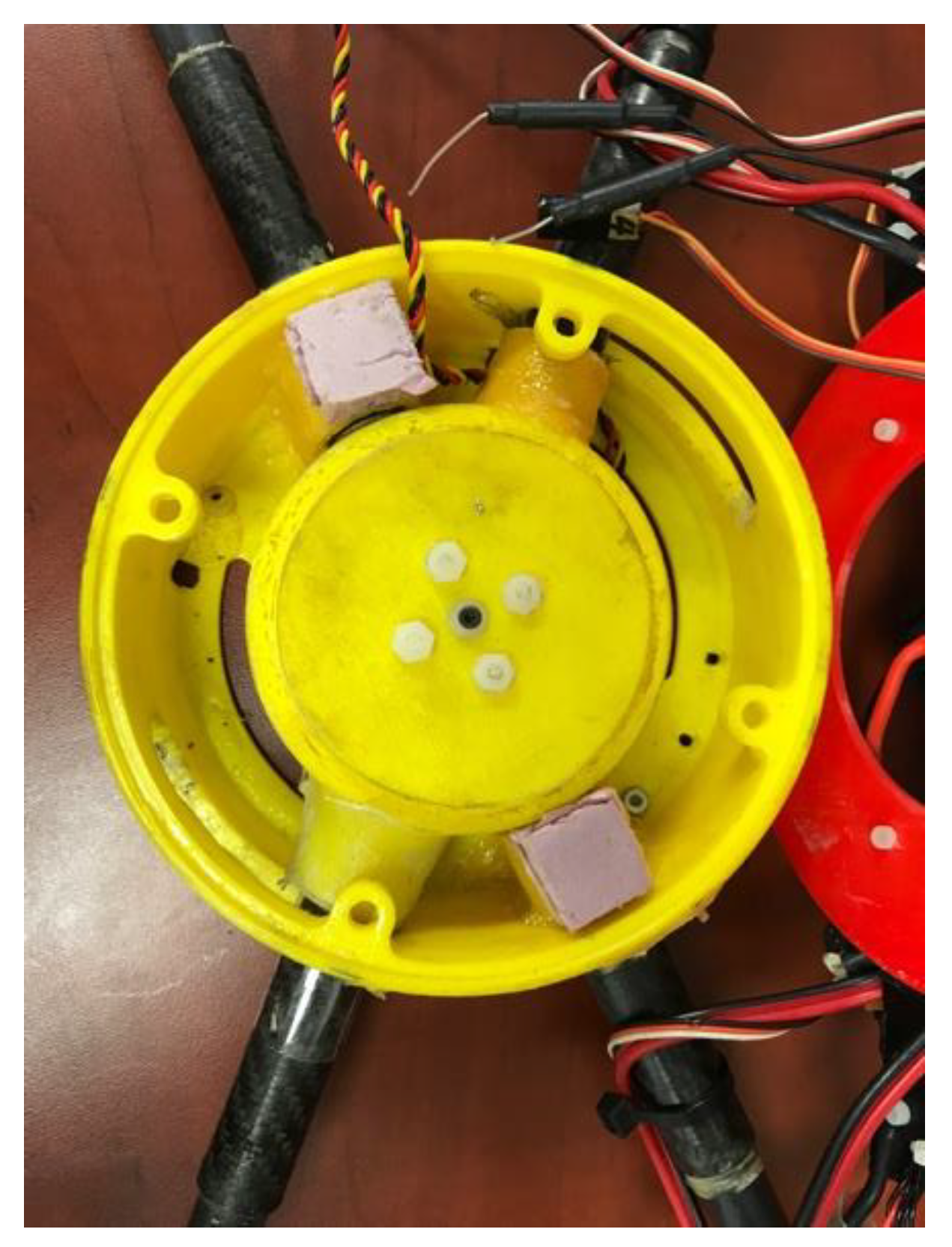
2.1.3. Fabrication of the Quadcopter and Morphing Mechanism
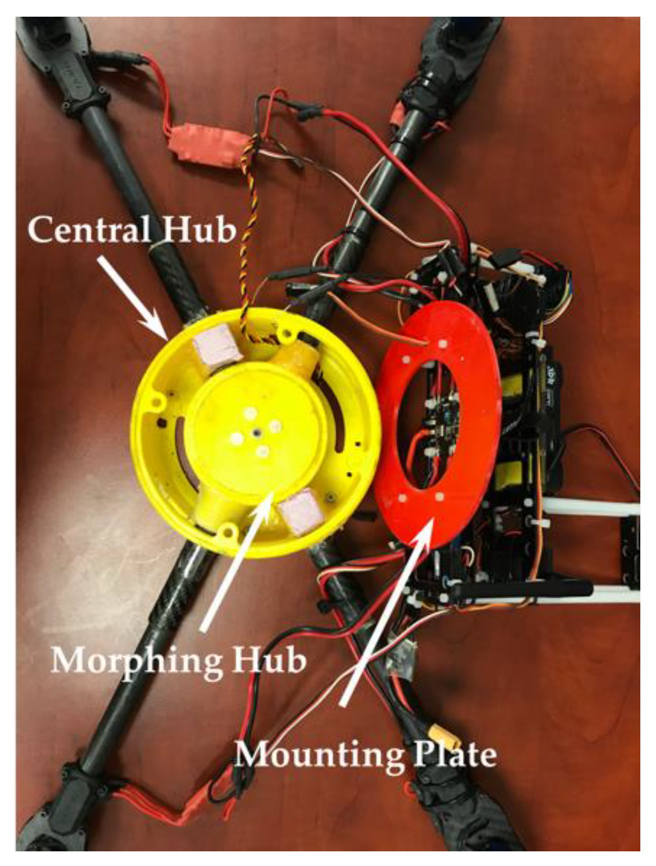
As was briefly mentioned earlier in this section, the quadcopter was designed with a central cylindrical hub with two co-axial cylindrical shells. The outer shell was designed to house the digital servo (HiTec HS-5625MG, [33]), whose drive shaft was connected to the inner shell. The outer shell featured mount points for two of the arms of the quadcopter, while the inner shell featured mount points for the other two arms of the quadcopter. This central hub was fabricated using additive manufacturing techniques, which allowed for a quick turn around in between iterations of the design and the ability to quickly replace the morphing platform in case of crashes. The fabricated hub is shown below in Figure 4 and Figure 5.
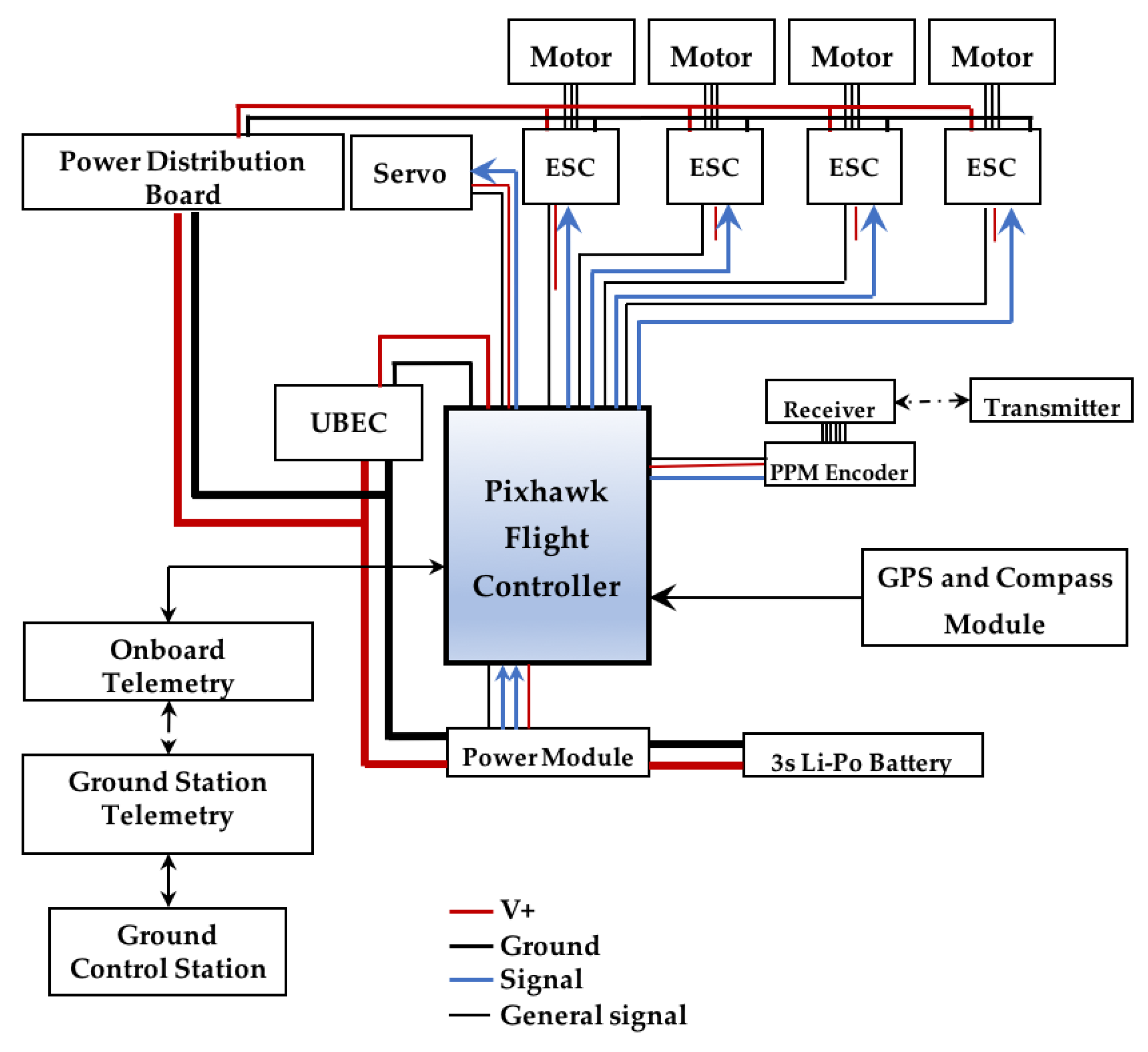
In order to power the servo driving the morping mechanism, an external battery elimination circuit (BEC) was used to provide sufficient input power on the servo rail of Pixhawk. This was necessary as the standard power module was only capable of powering the Pixhawk, receiver and the GPS module and not concurrently powering the drive servo. The specifications of the BEC are given in Table 3.
The finalized power distribution of the morphing quadcopter is illustrated in Figure 6 below:
3. Modeling of Quadcopter Moments of Inertia
The modeling and derivation of the equations of motion of a quadcopter are extensively addressed in published scientific literature, and can be found in the following references [34,35,36,37,38,39,40,41,42]. In the context of this experiment, the most critical aspect of the modeling of the quadcopter dynamics is in the derivation of the moment of inertia matrices for the nominal and morphed geometry configurations; in normal configuration, the quadcopter has a symmetric structure and so, the products of inertia are zero. On the other hand, morphed geometry results in an asymmetric configuration of the quadcopter, and consequently a change in the moments/products of inertia, particularly in non-zero products of inertia. In developing the inertia matrices for the normal and morphed configurations in this experiment, the following assumptions are made:
- i
- The model can be represented as two thin (massless) sticks intersecting at its center;
- ii
- The mass of the quadcopter is assumed to be concentrated at the ends of the intersecting arms, and are represented by point masses.
Based on these assumptions, the inertia matrix of the quadcopter, under normal geometry can be expressed as
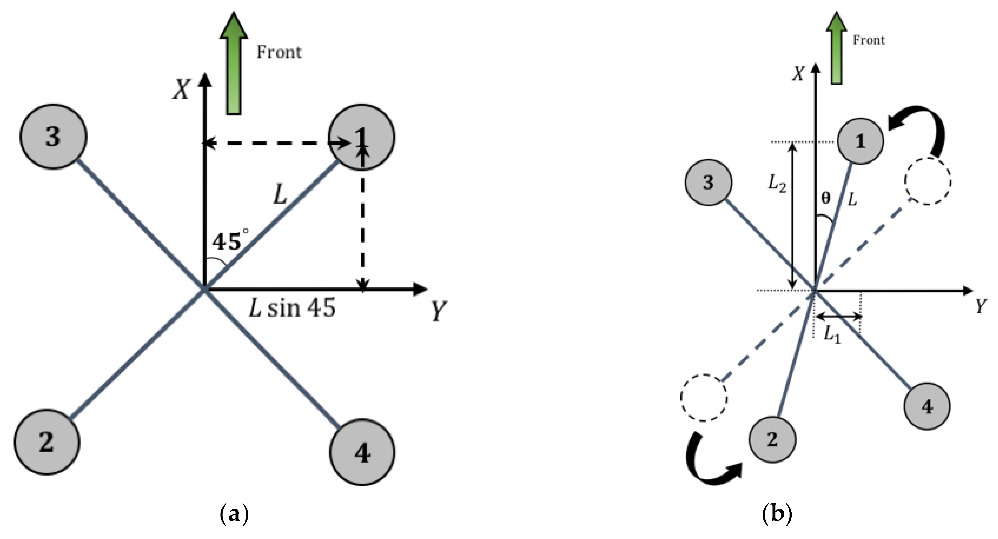
where , and are the moments of inertia about the , and body axes. Referring to Figure 7a for an illustration of the nominal configuration, these moments of inertia are determined as follows:
where is the mass of the point mass at the end of each arm, is the length of each arm, as measured from the center of the quadcopter to the shaft of the motor.
In the X-style quadcopter, the and body axes are not aligned with the arms of the quadcopter but point to the forward and lateral direction, respectively. In this configuration, any rotation of two arms of the quadcopter results in a change from a symmetric to an asymmetric structure about the body fixed reference frame, as can be seen from the illustration in Figure 7b. Note that the forward direction of the flight controller remains fixed even after transition to a morphed geometry. Also, as illustrated in Figure 7b, the angle represents the angle between the X-Axis and the arm supporting motors 1 and 2. It is the difference between nominal configuration and the angle of morphing. i.e.,
Thus, at a smaller morphing angle, the quadcopter is closer to its nominal configuration than it is at the larger morphing angle.
In the normal symmetrical configuration, the products of inertia are zero; however, a morphed geometry results in an asymmetric structure of the quadcopter, which affects the moments and products of inertia as well as the moment distance, and results in a non-zero product of inertia, and .
Under these conditions, the moments and products of inertia are given by the following expressions:
where L is the length of the arm.
In the case of morphed geometry, the moment of inertia matrix is given by
where is the moment of inertia of the morphed structure.
4. Simulation and Flight Test Experiments
4.1. Simulation of UAS Dynamics and Validation of Stability of under Morphed Geometry Conditions
It is necessary to evaluate the stability of different morphing geometries prior to executing complicated tasks such as the “Figure-8” flight path. In order to analyze the performance, the dynamics of the quadcopter were simulated within a custom developed Matlab simulation environment. The simulation was run using the same geometrical, physical and inertial parameters as that of the flight ready quadcopter. The parameters used in the simulation are listed below in Table 4.
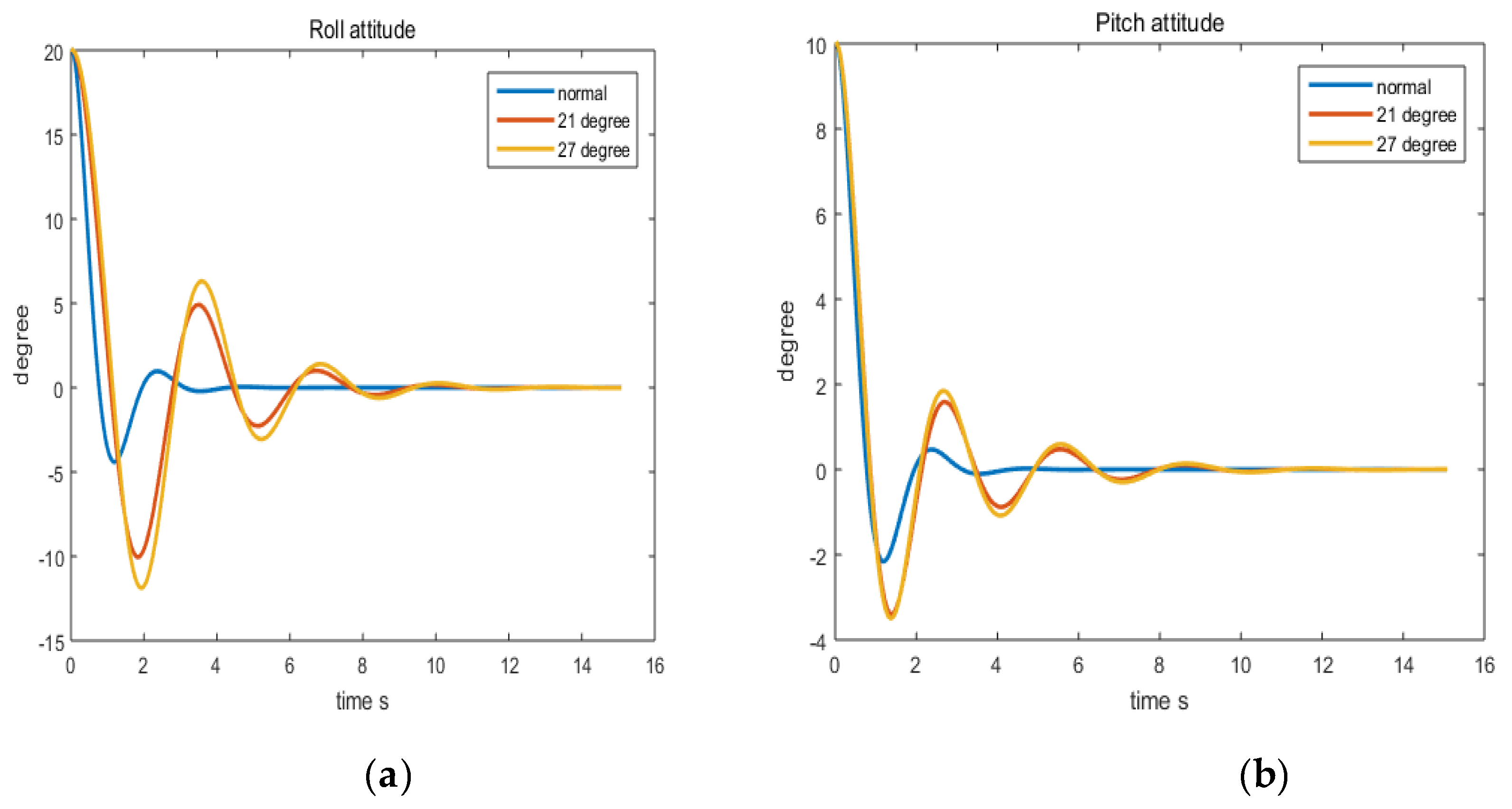
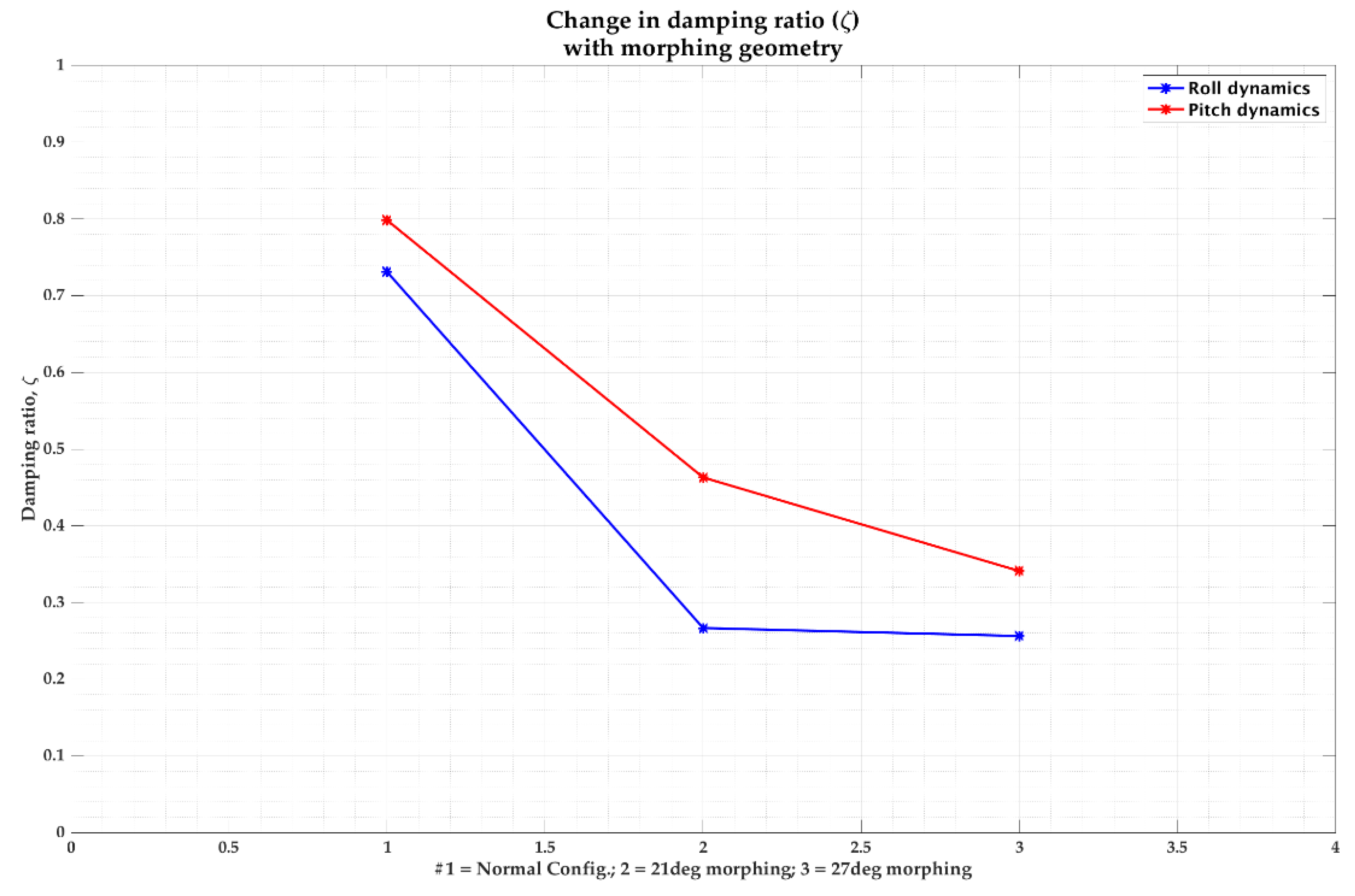
The response of the quadcopter to a step change in its attitude, under different morphing geometries is listed in Table 5 and plotted in Figure 8a,b below. Figure 8a represents the roll attitude response and Figure 8b the pitch attitude response. From the responses, it can be seen that at morphing, the quadcopter has less damping than at morphing, and in both cases significantly lower than the when under normal geometry. It can also be seen from the responses that the settling time increases with increasing morphing angle. The damping ratio corresponding to the second order roll and pitch dynamics of the quadcopter are shown in Figure 9—as can be seen clearly, from both Figure 8 and Figure 9, a change in the geometry of the quadcopter affects the lateral stability (roll) of the quadcopter more than the longitudinal (pitch) stability, and further, a small morphing () has a smaller effect than a large morphing ().
4.2. Flight Test Experiments
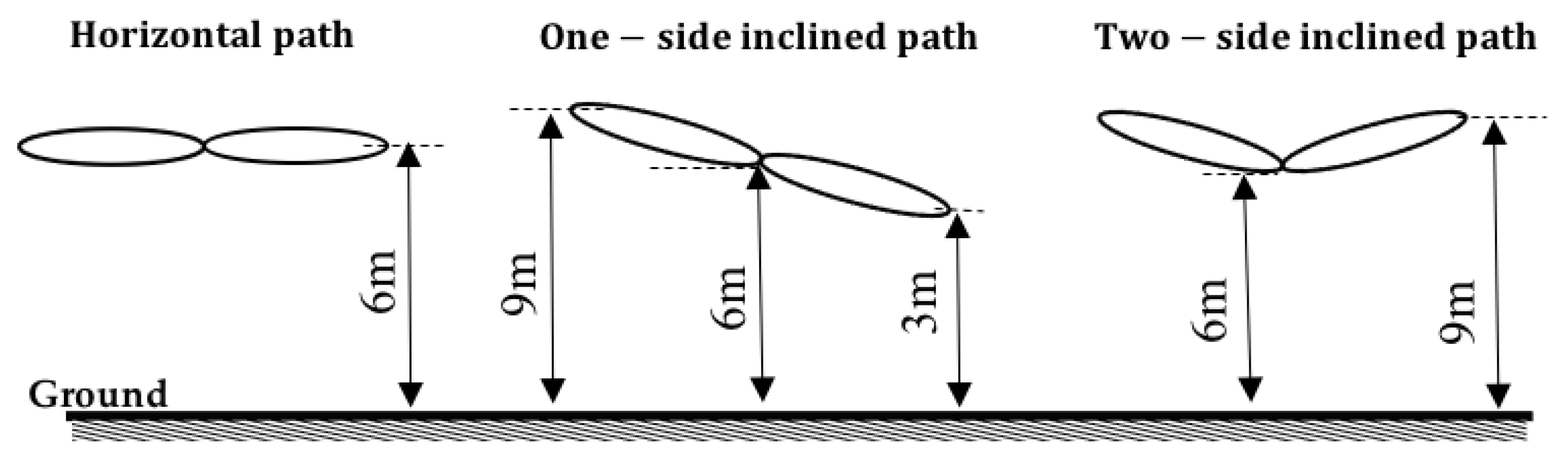
Following the validation of the stability of the quadcopter’s dynamic response under morphed geometry, the following experiments were designed to evaluate the performance of the morphing geometry quadcopter, while flying a “Figure-8” flight path. Each flight scenario (details of the flight test conditions are listed in Table 6) was repeated 10 times, following the steps described in Table 7, to ensure reasonably reliable statistics to assess flight performance. The “Figure-8” flight path was designed to be flown under different conditions by varying the velocity, number of waypoints, and angle of morphing. Due to limitations of the physical structure of the quadcopter (limitations imposed by the possibility of propeller overlap) the morphing angle was limited to and . In addition, the experiments were designed to include “Figure-8” flight paths in three different planar configurations: normal (single horizontal plane), single inclined ( inclined plane) and double inclined (the two lobes of the “Figure-8” were in two different planes inclined at from the horizontal plane)—these are illustrated in Figure 10 [43].
Each flight was flown similarly with manual take off, followed by autonomous flights from the center of the “Figure-8”, followed by a short hover (5 s) at the end of the flight, and landing, as described in Table 7 below. During autonomous flights, the pilot in command was always on standby to take over control of the quadcopter in case of abnormal behavior or other emergency situations.
4.2.1. Hover Flights, with Morphing
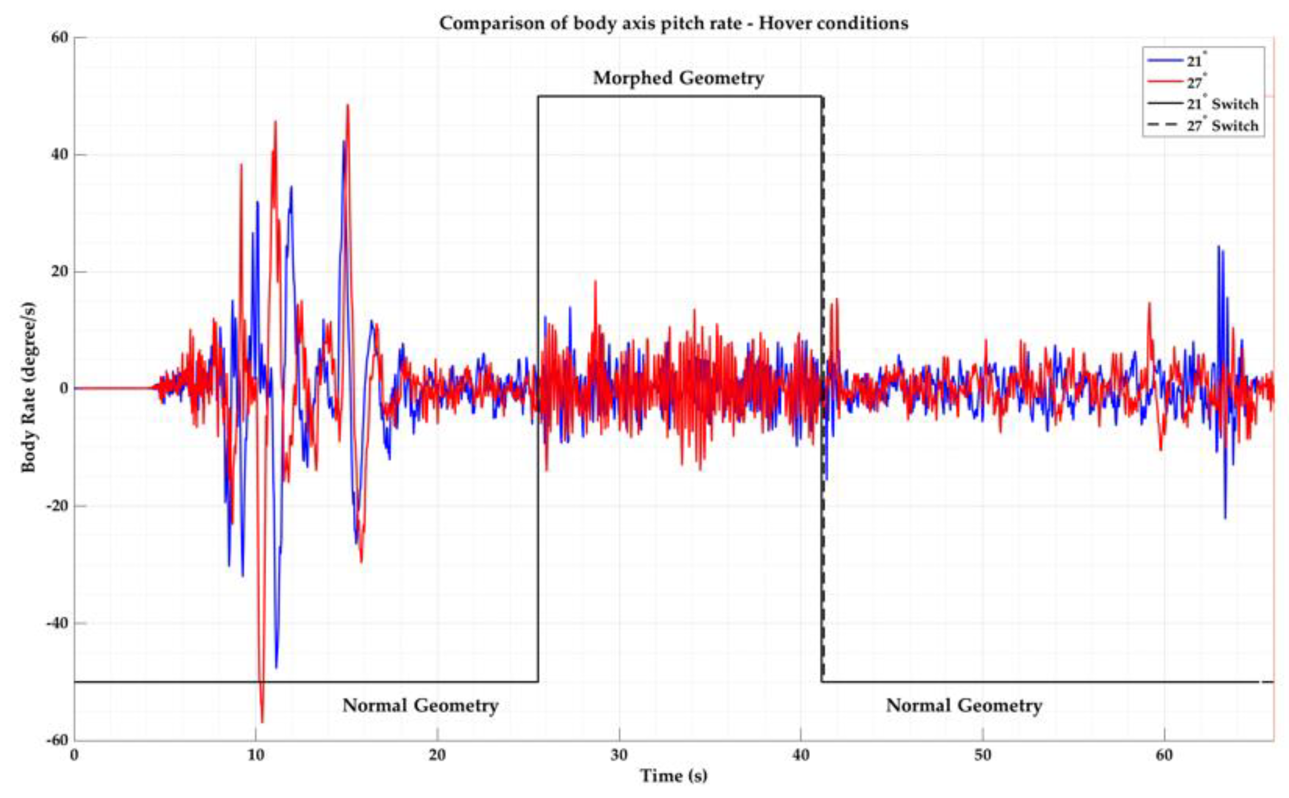
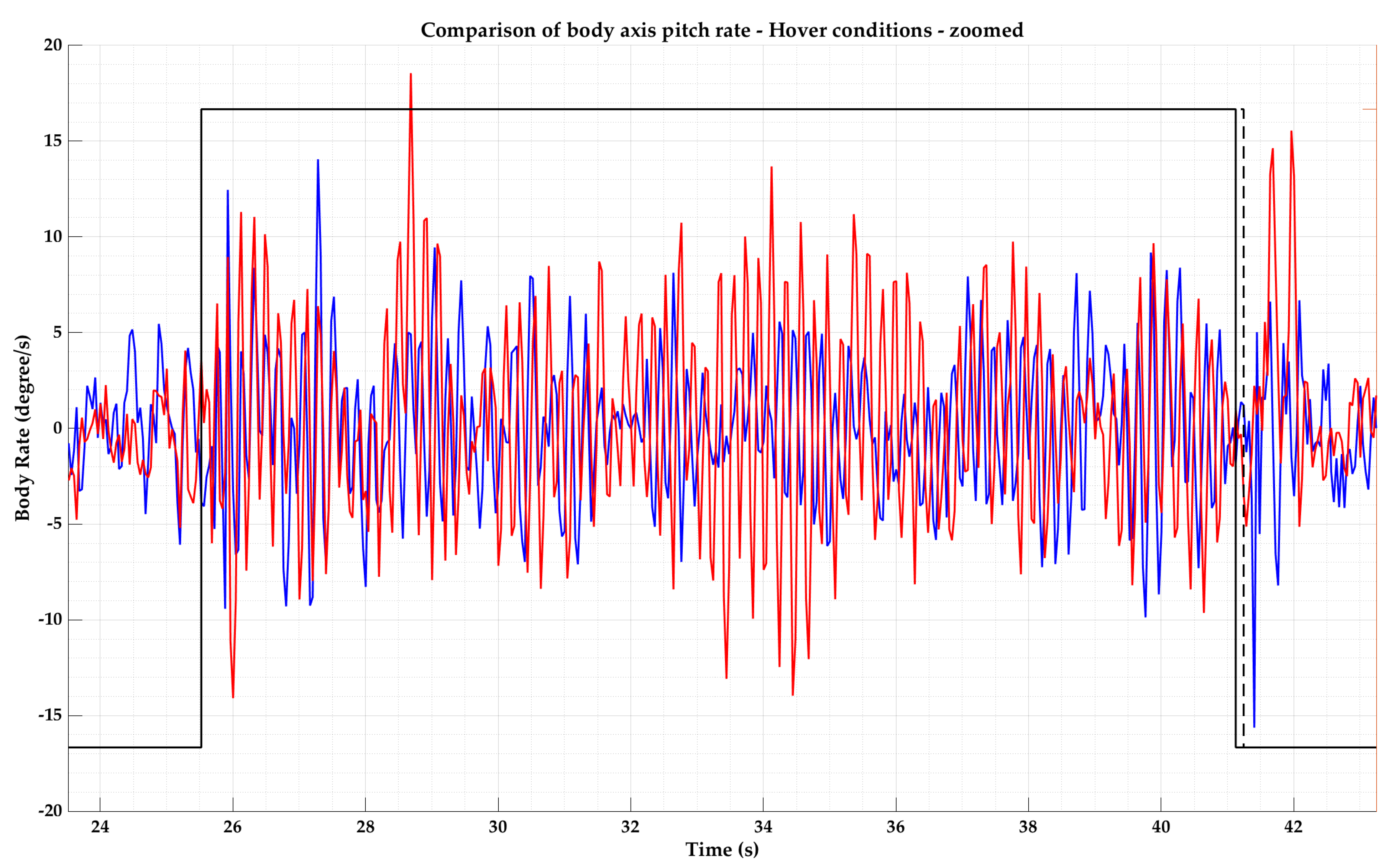
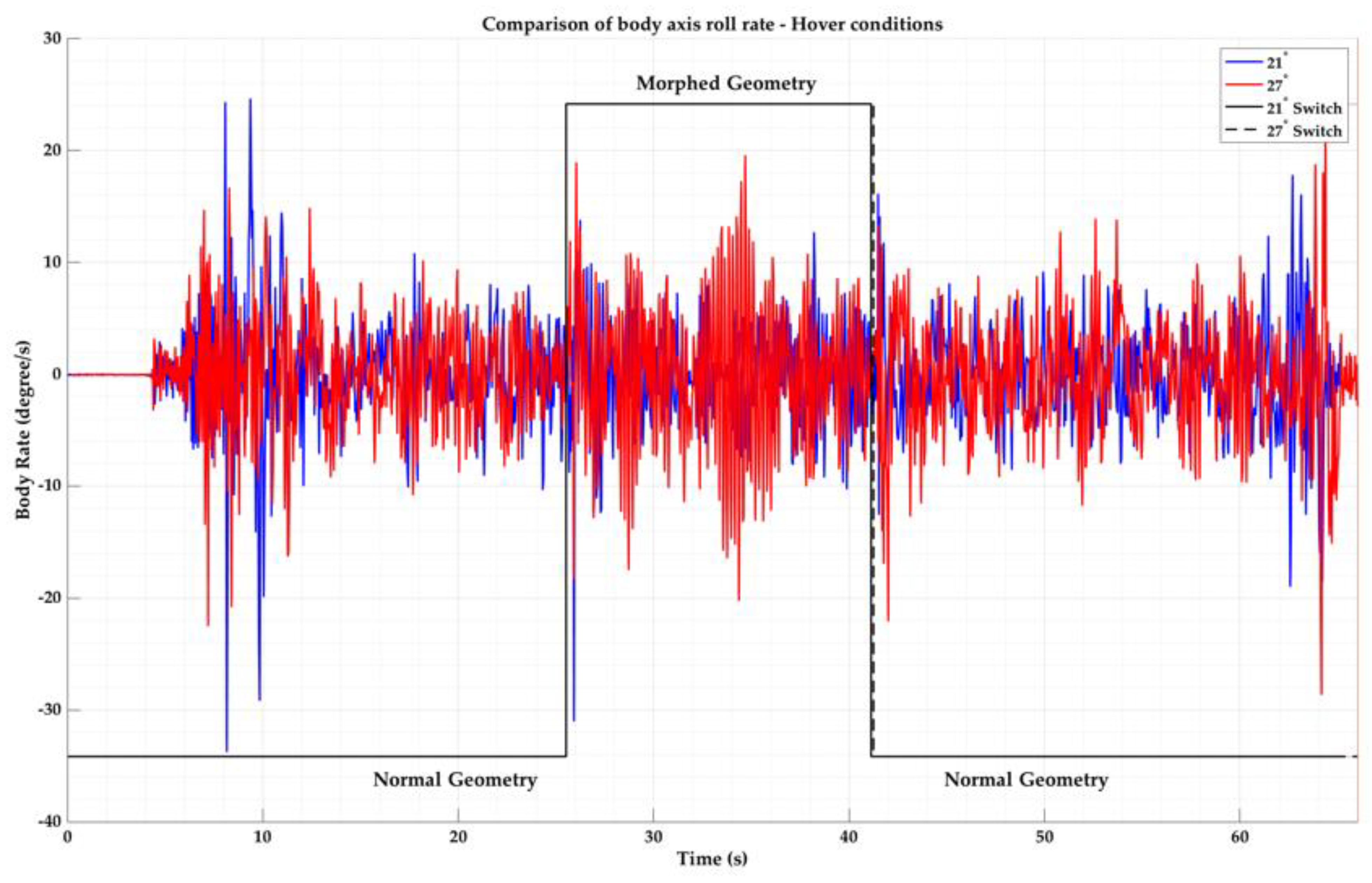
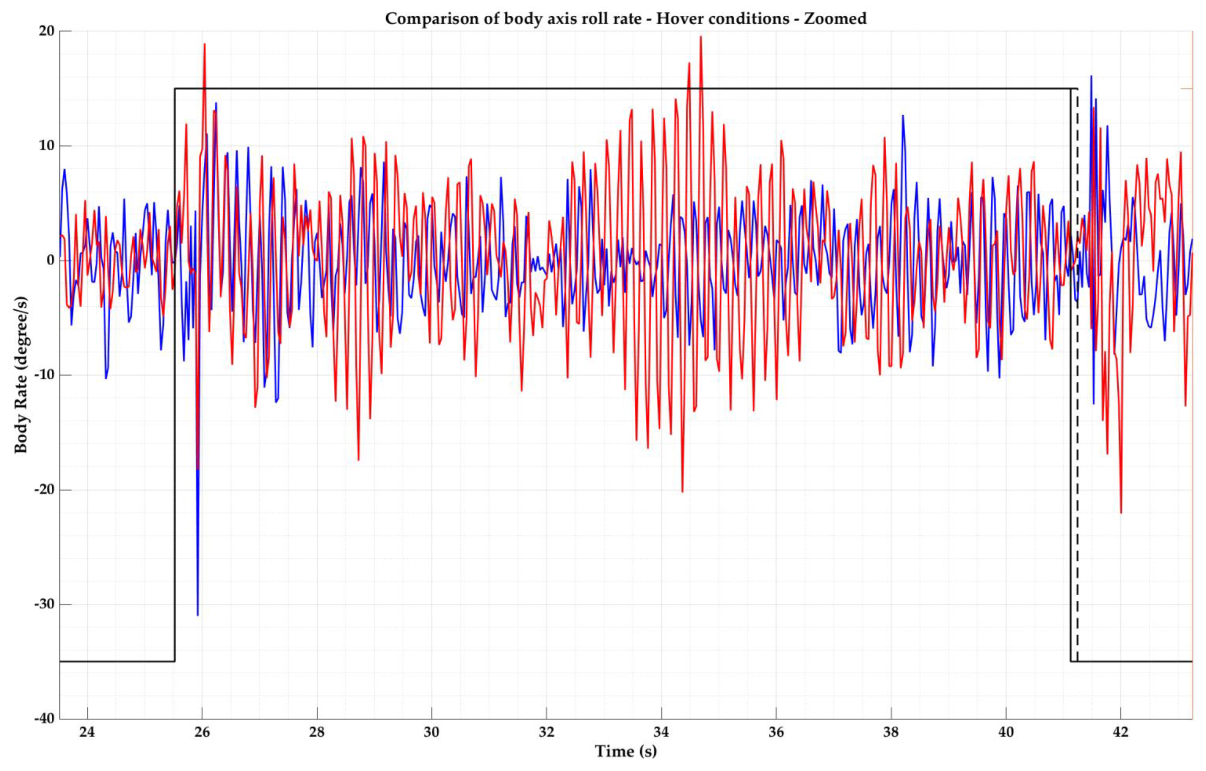
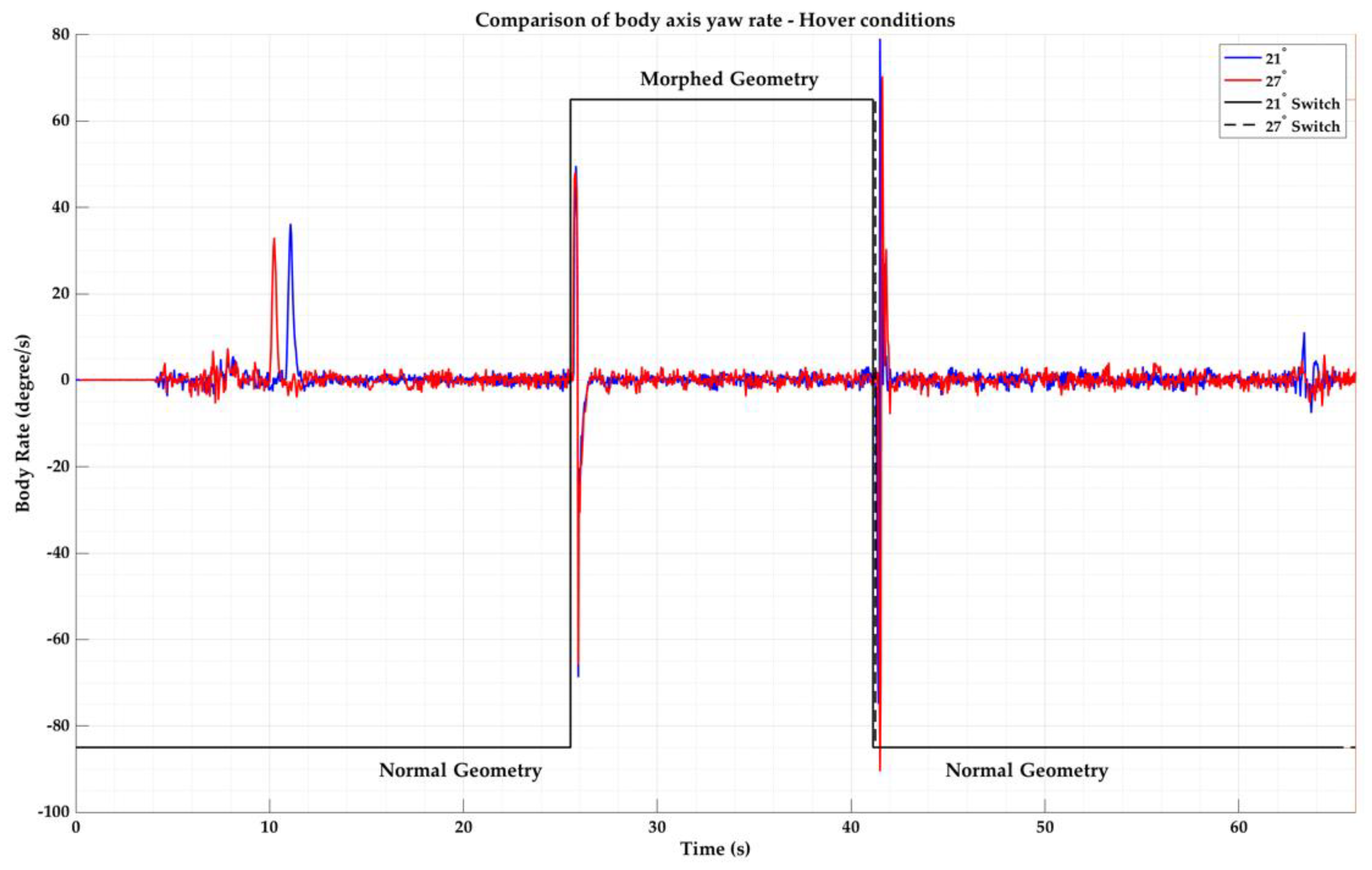
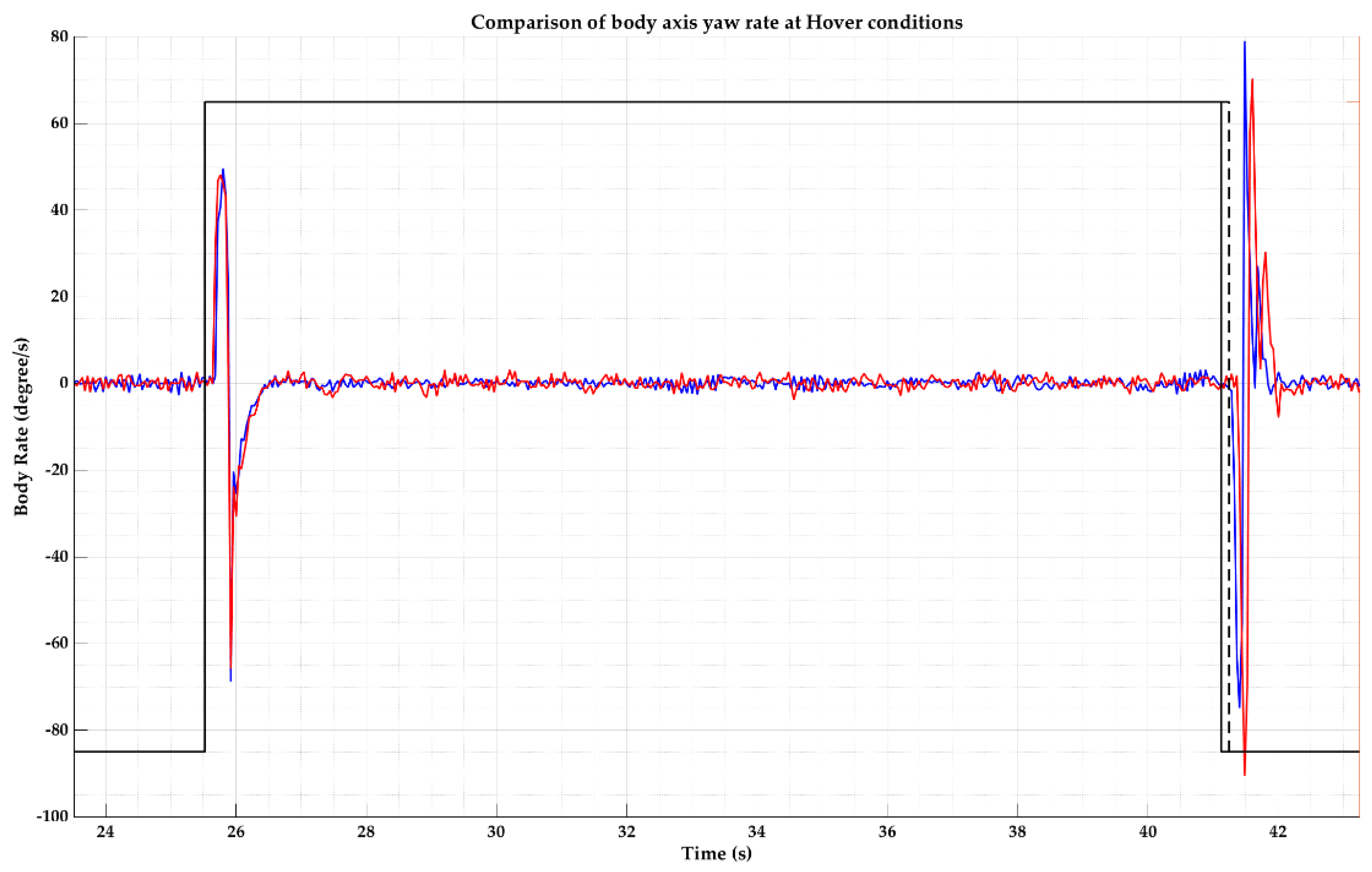
Following simulations, the quadcopter was tested under hover conditions, with morphing initiated, as the first step prior to full-fledged tests of the “Figure-8” flights. Following manual take-off and after reaching a desired altitude, the quadcopter was switched to the autonomous “position hold” mode and the geometry morphing was initiated to keep the new structure for approximately 15 s. This was followed by recovering its normal structure and landing (autonomous landing). The roll and pitch body axis rates during the and switch back from were analyzed under two conditions ( and ), and the responses are shown in Figure 11, Figure 12, Figure 13 and Figure 14 below. As can be seen from the figures, a larger morphing () results in a larger oscillation of the pitch and roll rate than morphing. As morphing does not affect moment distance and inertia related to the z axis, the yaw rates under both morphing conditions were relatively similar, considering the small differences in flight conditions, as is shown in Figure 15 and Figure 16.
Data from 10 flights of each morphing condition (, ) are presented below in Table 8. Note that in this article, flight performance worse than that in the normal geometry configuration is marked in red and flight performance better than that of normal geometry is marked in green.
From the table, it is clear that the mean values of the averages are very close to each other—as few conclusions can be drawn. On the other hand, the standard deviation of all the angular rates (mean of the 10 runs of roll, pitch, and yaw rates) during hover show an increasing trend with increasing morphing angle, indicating higher oscillations around the mean value and a reduction in dynamic stability. On average, the larger morphing angle resulted in an approximately 1.5-fold increase in the standard deviation of the angular rates (roll and pitch) as compared to the smaller morphing angle. This could be attributed to the fact that a large morphing angle decreases the damping ratio of the system dynamics more, as compared to a smaller morphing angle.
4.2.2. Figure-8 Flights, with Morphing
The primary goal of this effort was to determine the flight performance of the quadcopter in various morphing configurations, while performing a complex mission; as previously described, 10 flights of the “Figure 8” trajectory were executed in each configuration (morphing angle, #of waypoints, velocity and plane). Also note that the following flight conditions had a different number of flights than the standard 10 sets:
vel. = 1.5 m/s; wp = 30; morph = ; horizontal plane: 11 flights
vel. = 2.5 m/s; wp = 20; morph = ; horizontal plane: 9 flights
vel. = 2.5 m/s; wp = 30; morph = ; horizontal plane: 11 flights
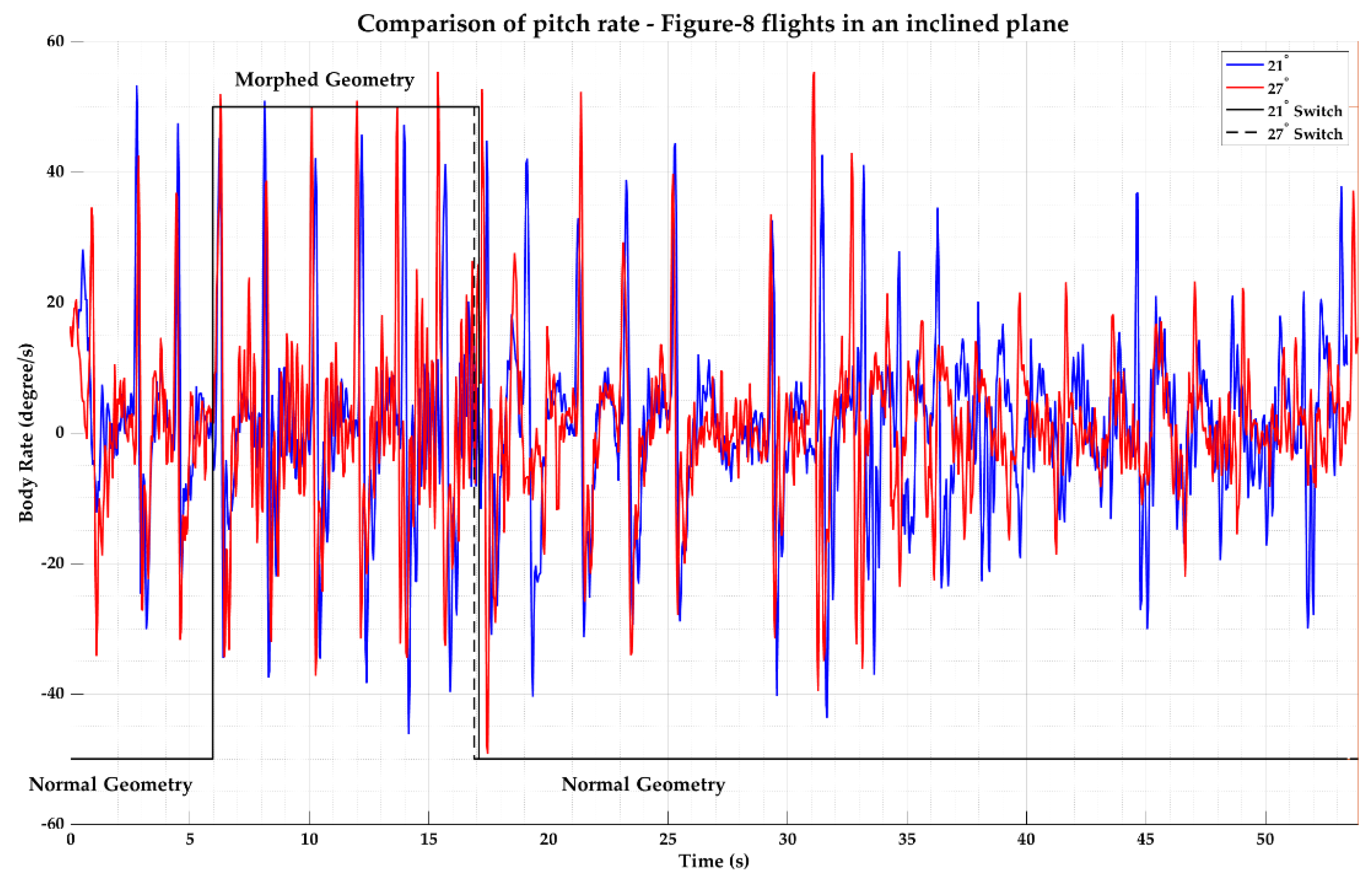
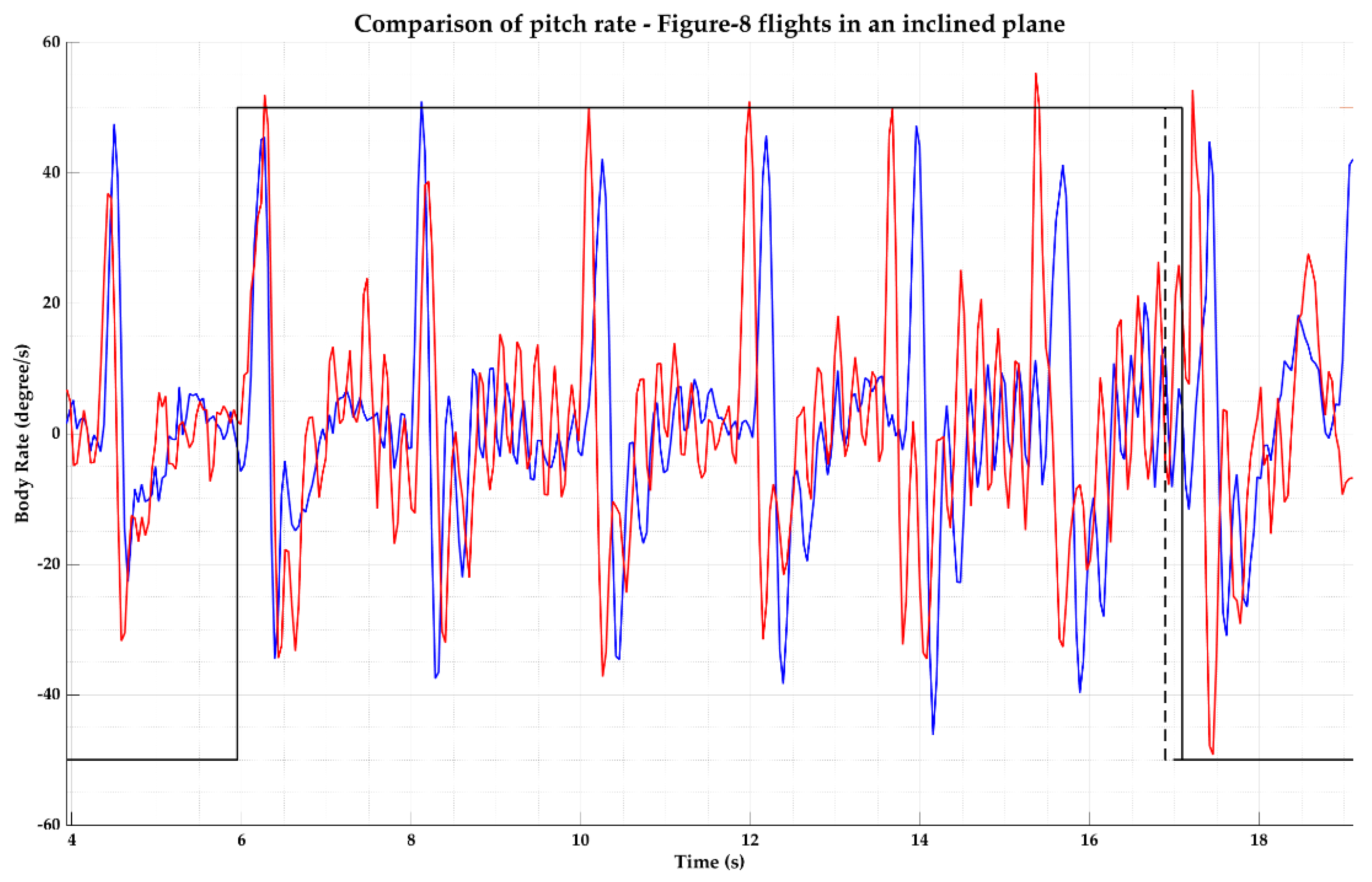
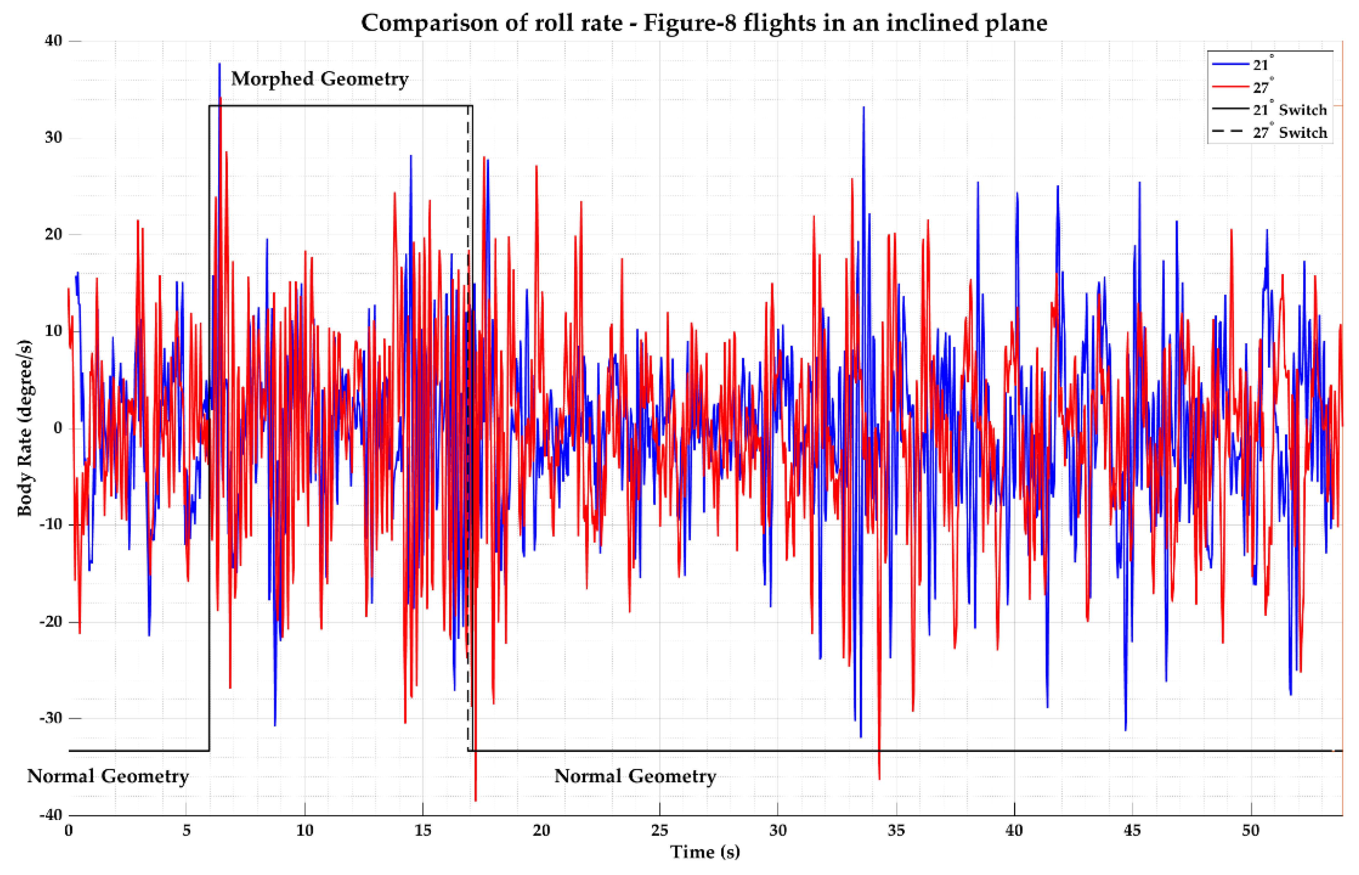
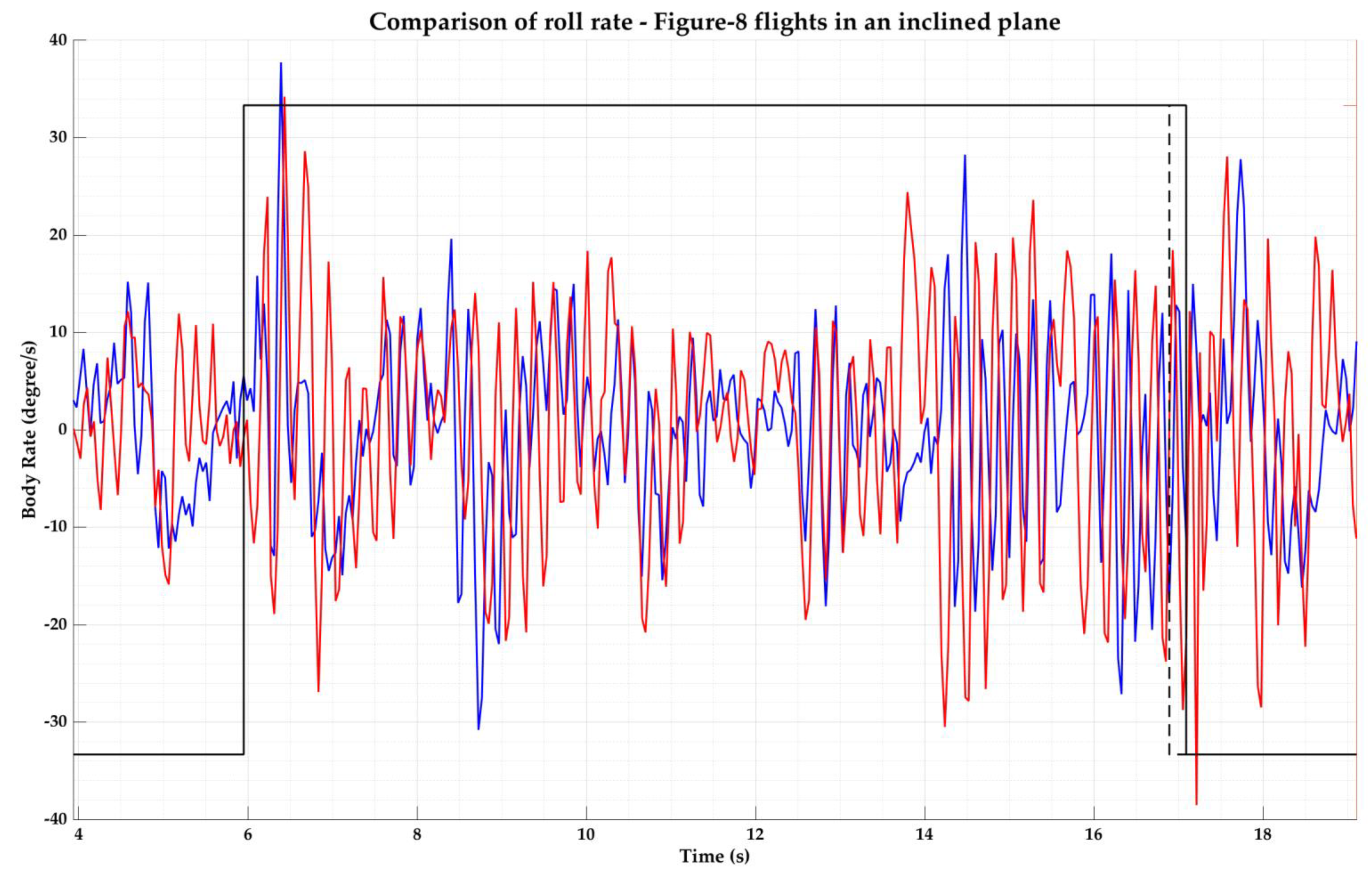
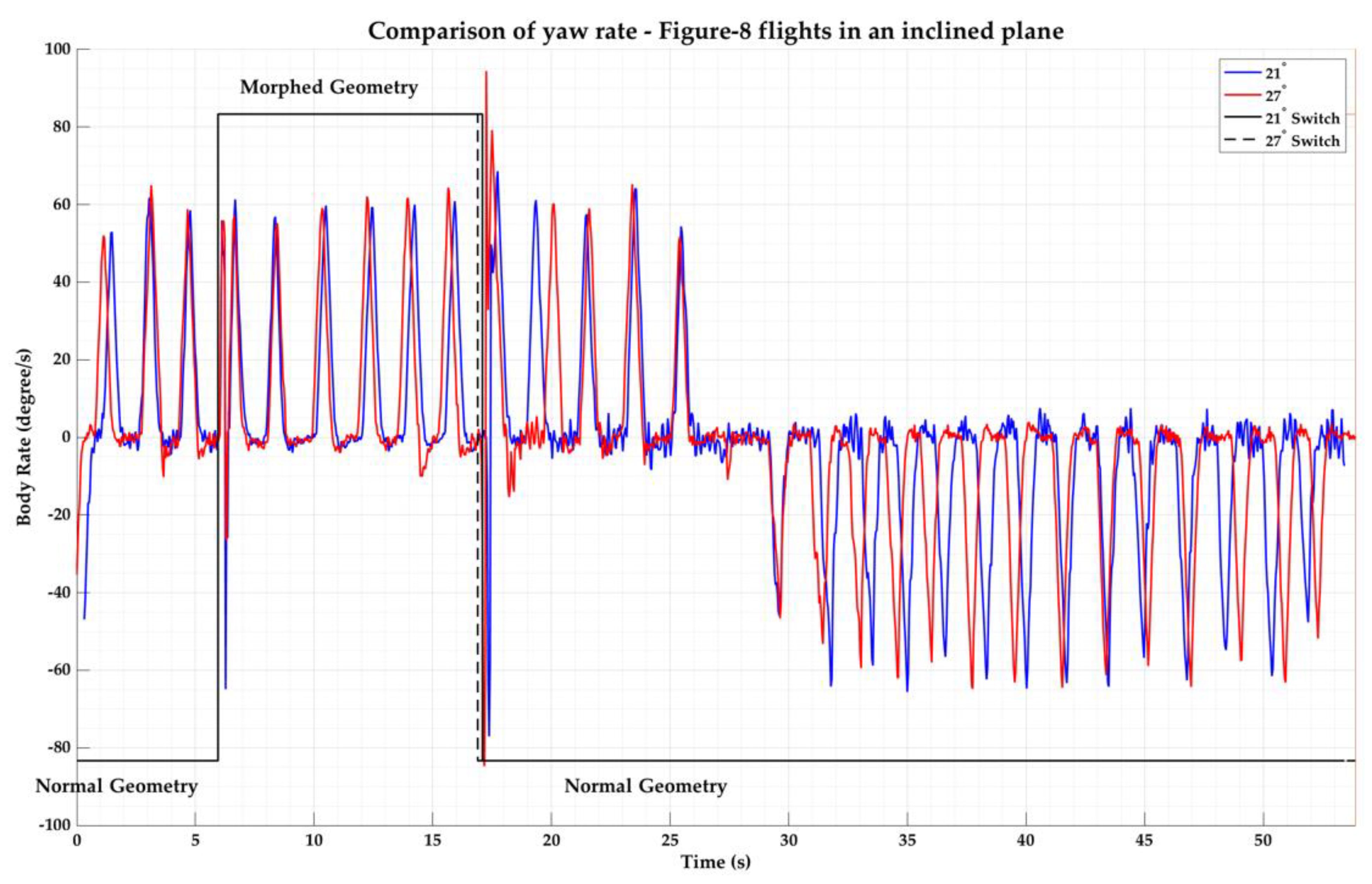
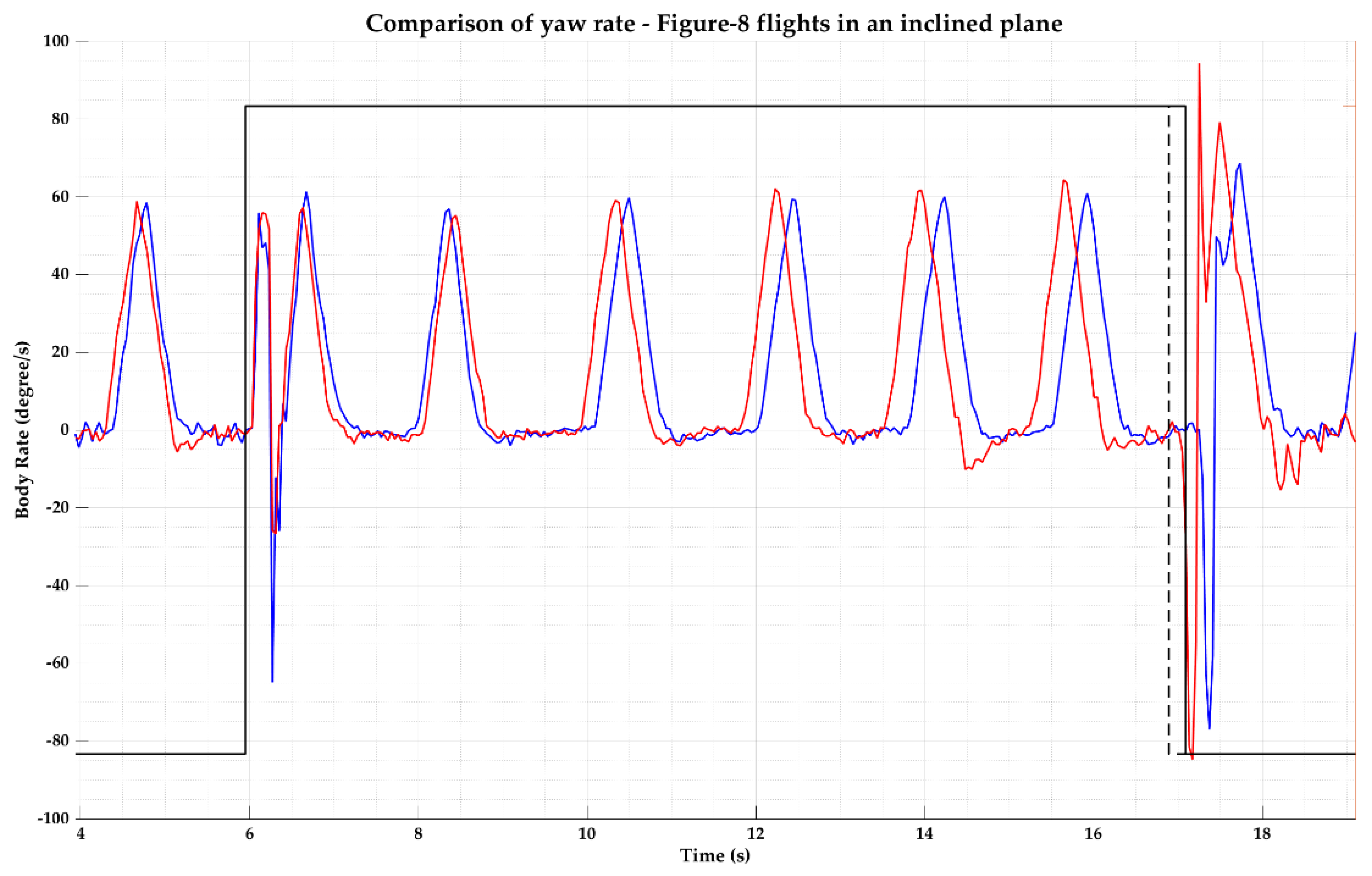
During these flights, geometry morphing was active only between two morphing waypoints (as listed in Table 6), and consequently, the body axis angular rates are analyzed only within this segment of the flight path. For comparison, results of small morphing (), and large morphing () are compared to normal geometry (), in different missions. The dynamic response of the quadcopter (at velocity, 30 waypoints, single inclined plane and and morphing) is shown in Figure 17, Figure 18, Figure 19, Figure 20, Figure 21 and Figure 22 below, for reference:
The standard deviation of the body axis angular rates of the quadcopter from the “Figure-8” flights in the segments with morphing geometry active are tabulated in Table 9, Table 10, Table 11, Table 12, Table 13 and Table 14.
From the data, it can be observed that the standard deviation of the roll rate of the quadcopter during the morphing flight segments are consistently larger under all flight conditions (# of waypoints, velocity and plane) than the corresponding value under normal geometry flights. Additionally, it was also observed that both the number of waypoints and the velocity had a significant effect on the roll rate—the performance of the quadcopter under morphing was consistently better than that under morphing by approximately 10% for the flight path with 20 waypoints at the lower velocity (1.5 m/s), and at a higher velocity (and 20 waypoints), the difference was more pronounced with the morphing condition performing 2–5 times better than the condition.
In the 30 waypoints flight condition, the morphing condition performed better than the two out of three times (in the inclined and double inclined plane) at the lower velocity (1.5 m/s). At the higher velocity condition, no significant difference was found in the performance (different morphing configurations) in all planes (horizontal, inclined and double inclined). From the data, it can be seen that under 20 waypoints and 1.5 m/s flight condition, the pitch rate follows the same trend as the roll rate—the morphing angle has smaller oscillations as compared to the morphing, although the magnitude of the differences between the two are not as pronounced as that for the roll rate. Except for one flight condition (, 1.5 m/s and inclined plane), under all the other flight conditions the difference from the baseline performance was within . In the case of yaw rate, while there were some observed differences between the morphed geometry conditions and normal flight conditions, it was within of the baseline performance.
The differences between the pitch and roll rate responses are consistent with the fact that morphing reduces the damping ratio of the roll dynamics more than that of the pitch dynamics. Additionally, the variations in the performance of the roll rate response in different morphing configurations and flight conditions— performing better in some cases than and vice versa, could be attributed to uncontrolled/unaccounted factors, including environmental conditions and artefacts of the physical structure of the UAS, especially in the connections between the arms of the quadcopter and the central hub.
4.2.3. Position Error
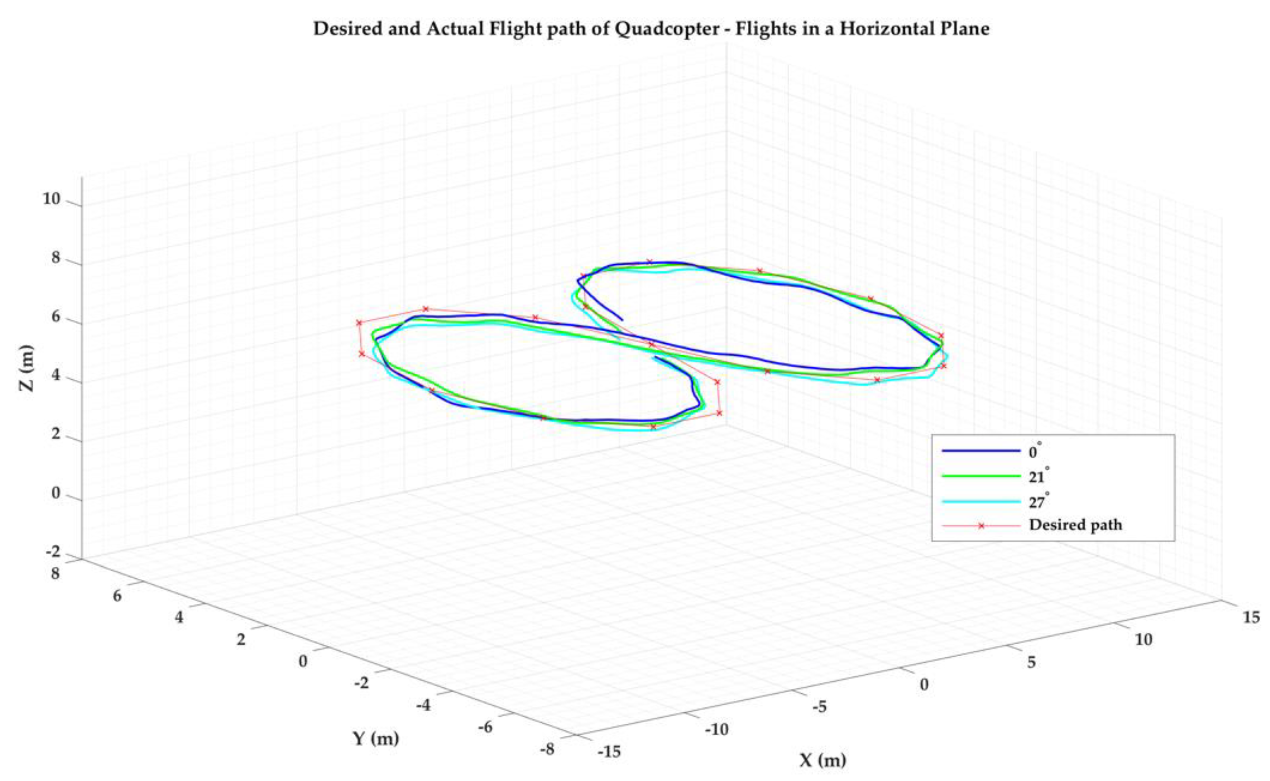
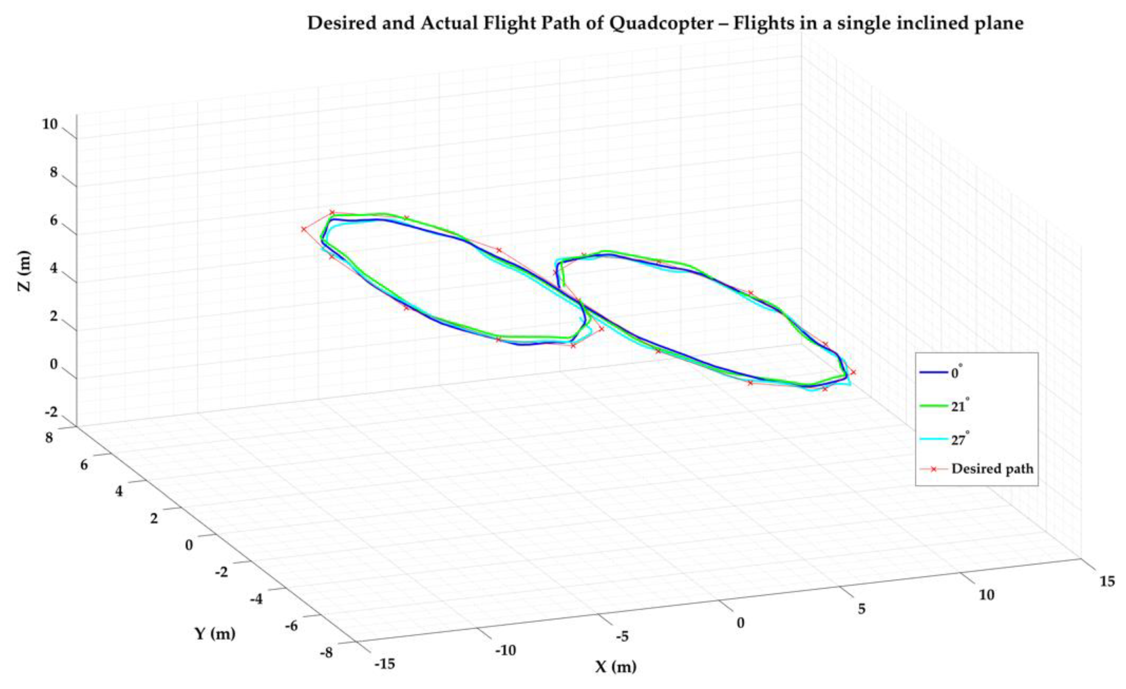
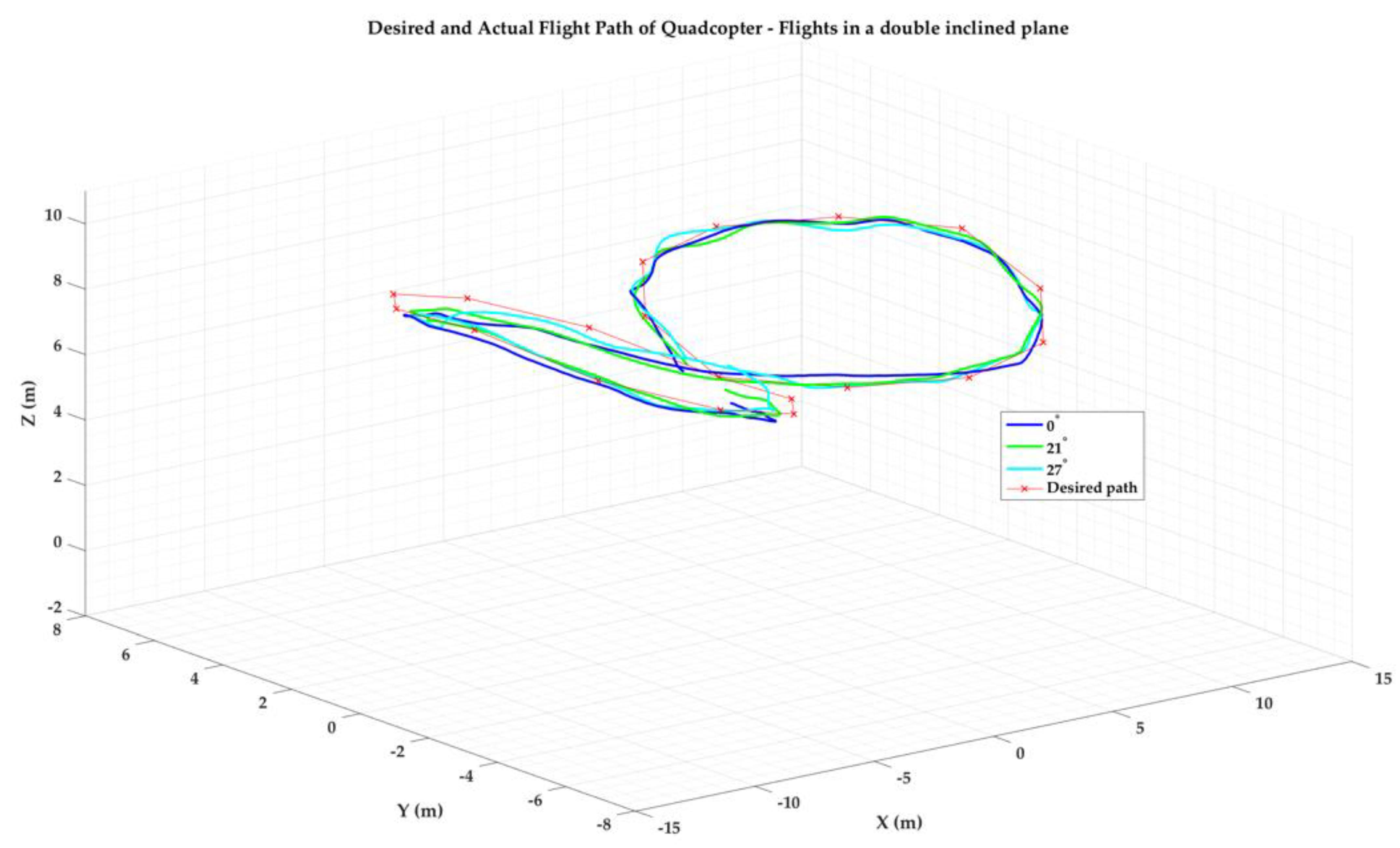
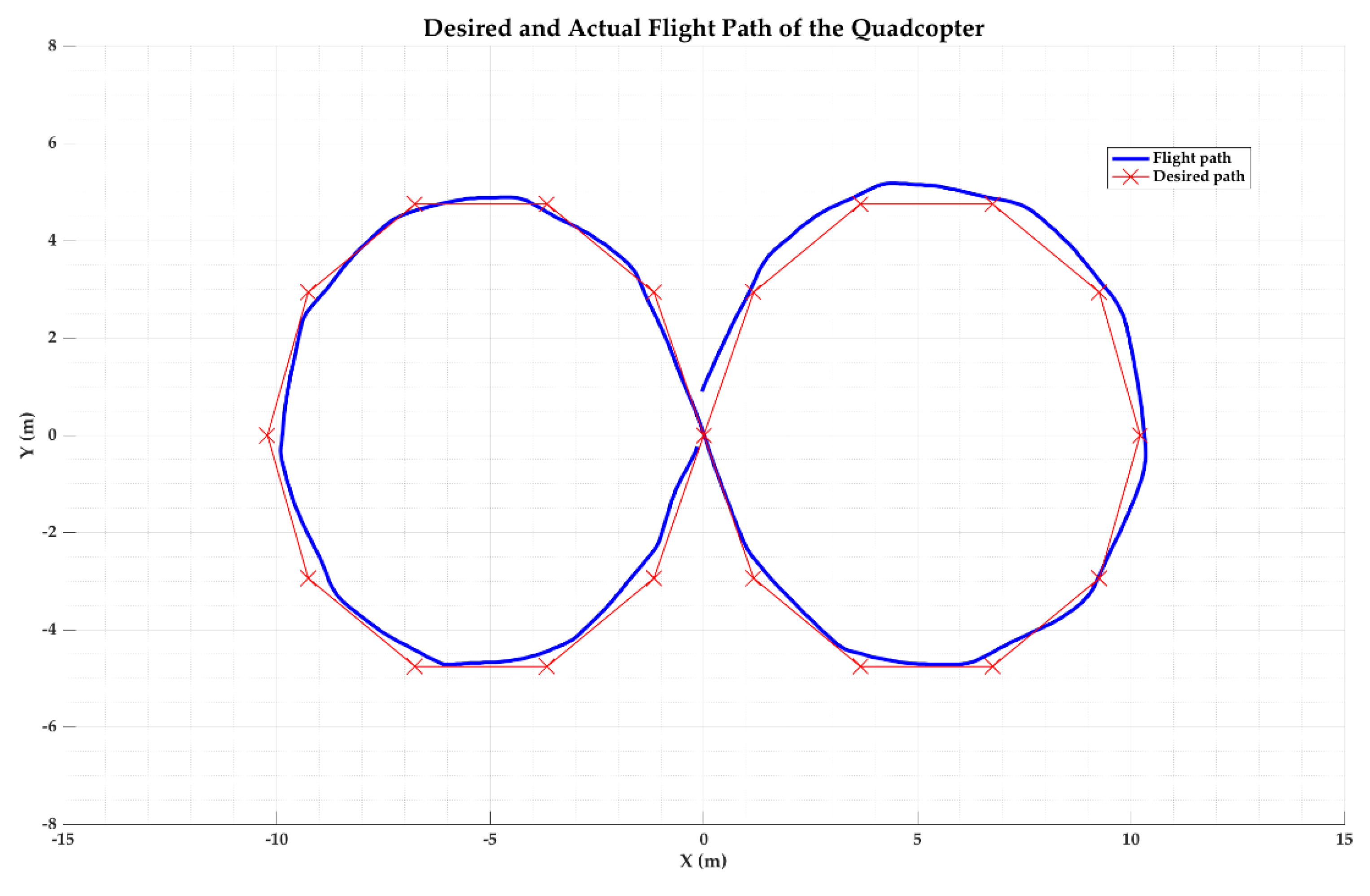
In addition to the analysis of the quadcopter’s angular rate responses during the morphing process, we also considered the overall performance of the quadcopter in following the desired flight path, with and without morphed geometry. In order to accurately assess this performance, it is critical to parse the flight data into appropriate segments between the waypoints that the quadcopter is programmed to fly through in a designated sequence. In our experiments, the drone is designed to start at the center of the “Figure-8”, fly through the two lobes of the “Figure-8” in both clockwise and counterclockwise directions, return to the center of “Figure-8” before landing. Sample 3D flight paths flown by the quadcopter are shown in the Figure 23, Figure 24 and Figure 25 below.
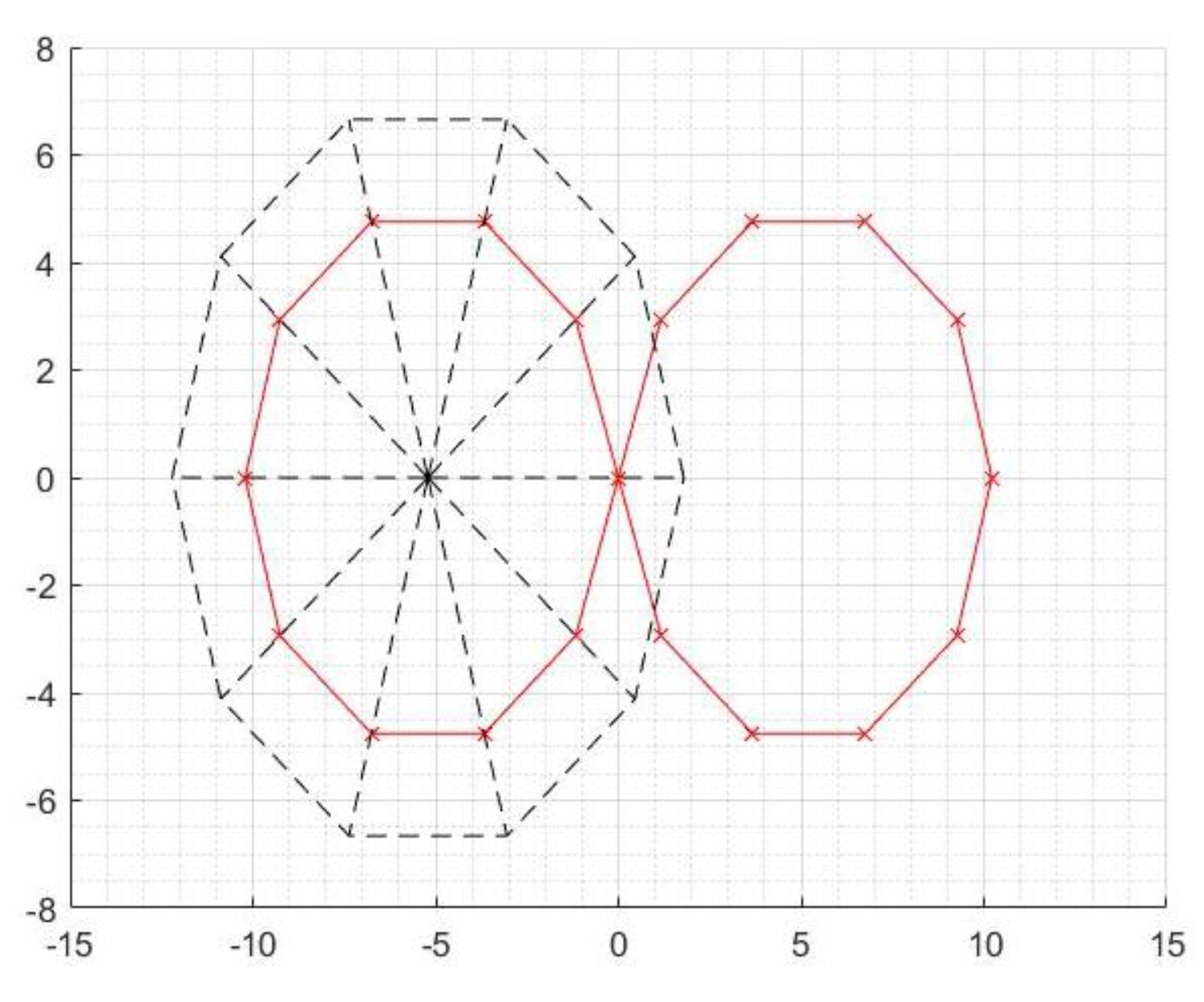
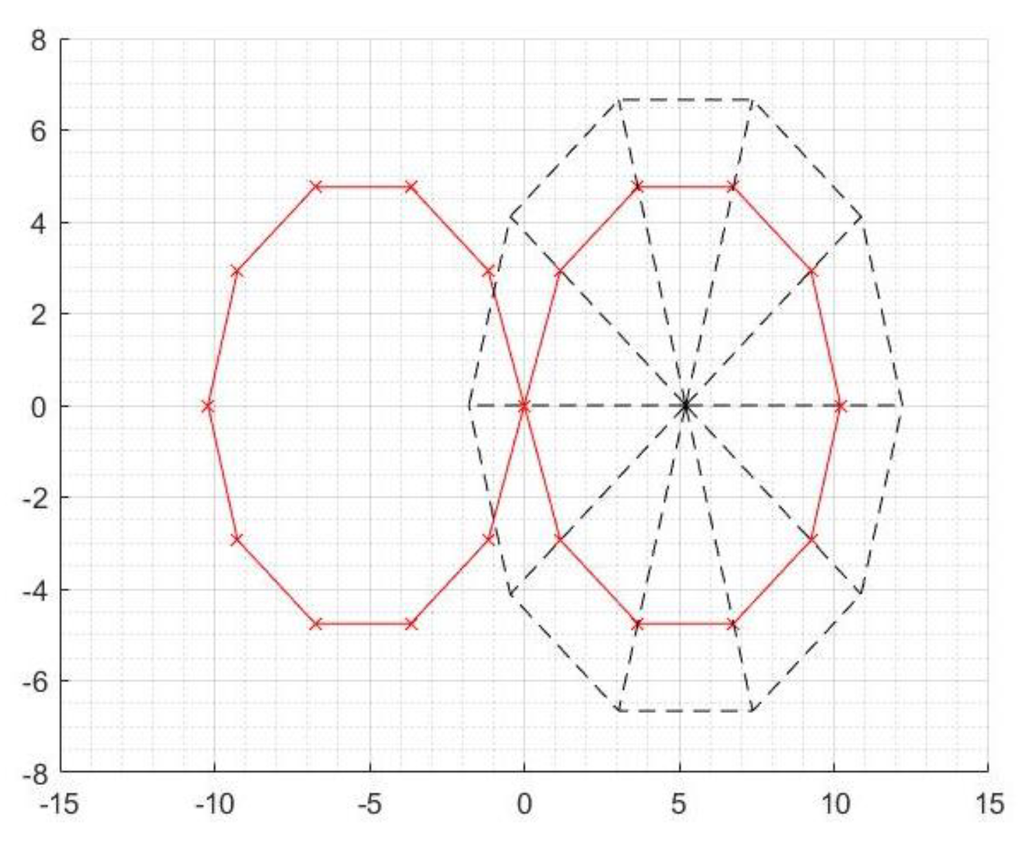
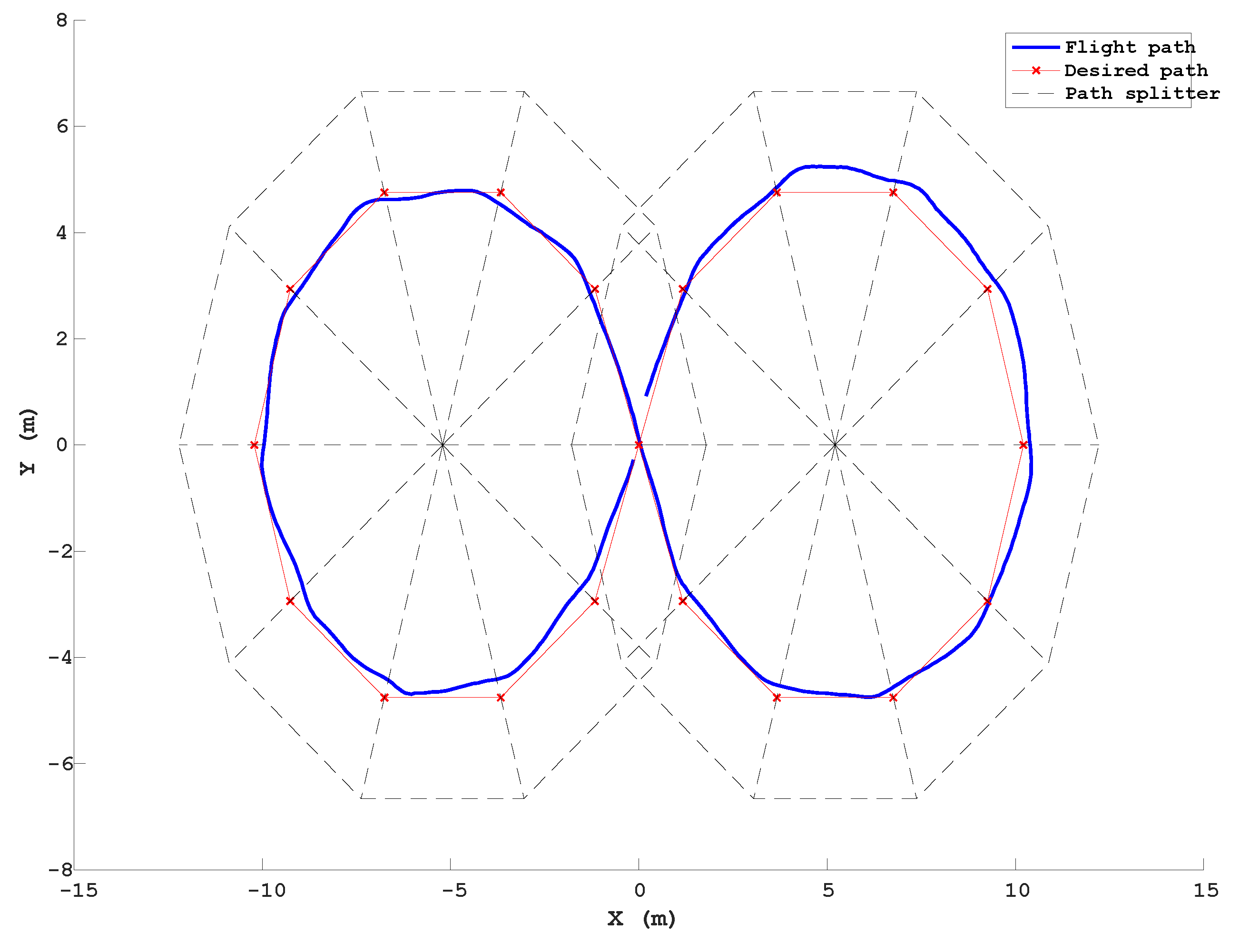
4.2.4. Splitting the Trajectory into Appropriate Segments Using a “Sliced Pie” Concept
In order to evaluate the performance of the quadcopter in following the desired flight path under both normal flight and morphed geometry, we introduce a method to split the “Figure-8” flight path data and analyze the position error. We term it the “sliced pie” method—similar to cutting a pizza pie into several slices. In this method, the trajectory is split (sliced) to correspond to segments between two consecutive waypoints. We then evaluate the position errors along each segment of the desired trajectory as the mean error of the recorded GPS trajectory from the desired straight-line segment. The process of splitting the trajectory into segments is as described in the Table 15.
4.2.5. Method of Triangles to Identify the Segments of Flight Path
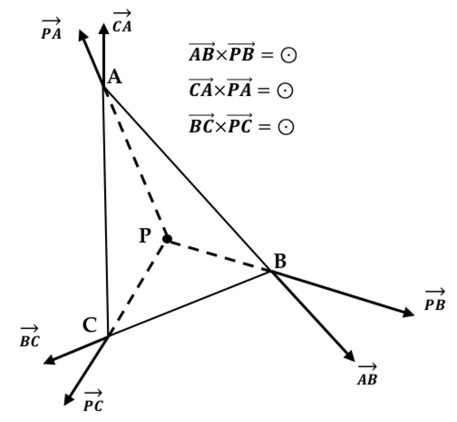
Following the generation of the “sliced pie”, it is necessary to confirm whether a segment of flight path (GPS location of the UAS) lies within the region covered by the current pie slice or not, to be enable generation of trajectory position errors. In order to do so efficiently, we use the concepts of vectors and vector cross-products.
Assume that the current GPS location of the UAS and the pie slice are represented by and , respectively. Six vectors related to the vertices of the triangle, , and the GPS location are represented as , , , , , respectively. If the point lies within the triangle , the direction of the cross product of the vectors , , and should all be out of the plane . On the other hand, if the point lies outside the triangle , the direction of the cross products will be into the plane, .
Numerically, assume all three coordinates vectors are in the plane of , which leads to the value of the coordinate of each vector being zero. After calculating the cross product, if the value of the coordinate of each result is all positive, it is indicative that the point lies inside the triangle . On the other hand, if one of the results are negative, it is indicative that the point lies outside of . In a marginal condition, is on one of the sides of , resulting in a zero value. This process is illustrated in Figure 30 and Figure 31 below.
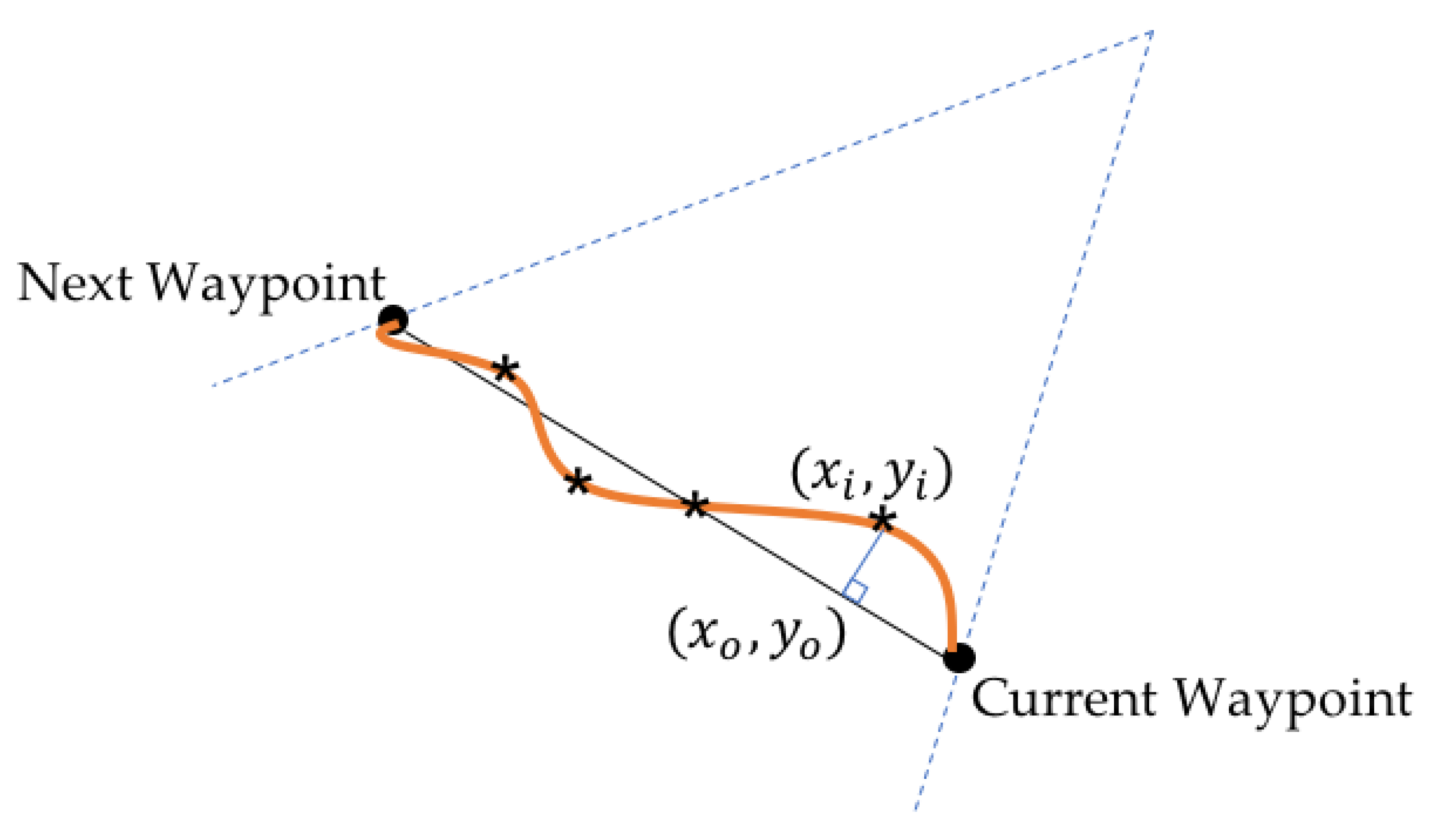
Since the quadcopter was programmed to execute the figure of eight path by flying in straight lines between waypoints, the accuracy of the flight trajectory was determined by calculating a trajectory error between two subsequent waypoints as the normal distance between each GPS point and a corresponding desired location between the waypoints. It is important to note that this trajectory error depends on a number of different factors, including the state of the battery, accuracy and stability of GPS signal, wind disturbance, reliability of the quadcopter’s structure, and morphing. In order to determine this trajectory error while flying between waypoints, in each segment, the desired position related to the current position (Figure 32) can be calculated as follows:
Based on two consecutive waypoints of a segment, a straight line connecting the waypoints can be expressed as:
If is the current GPS coordinate of the UAS, then another line, normal to the line , passing through can be written as:
The point of intersection of the two lines is the desired GPS coordinate that the UAS should have been at; it can be determined as . This would allow the calculation of the distance from the desired GPS location.
We consider this distance metric as the error in the trajectory of the UAS and the standard deviation of the trajectory error under all the flight configurations and flight conditions (mean value of the results of 10 runs of each flight condition) is listed below in Table 16. As can be seen from the table, the trajectory error is a mixed bag; in the morphed geometry flight condition, some flights (5 out of 12) exhibit a better tracking performance as compared to the baseline flights (normal geometry) while, for rest of the flights, the trajectory error is within of the value under normal geometry.
In the morphed geometry flight condition, the trend is similar; some flights exhibit a better tracking performance (4 out of 12) as compared to the baseline flights (normal geometry), while for rest of the flights, the spread is wider as compared to the configuration, with the maximum value of . It should be noted that for flights with a better performance than normal geometry, the improvement is not significant, with a maximum of . Some of these performance gains could be attributed to unrecorded factors, such as environmental conditions, wind gusts, or GPS coverage.
5. Discussion and Conclusions
In this article, we describe the fabrication and flight tests of a quadcopter capable of morphing its geometry in flight by changing its intersection angle. The quadcopter can morph from a nominal geometry to two morphed conditions, and —the limits allowed by its physical dimensions. The morphing is facilitated by a digital servo driving a 3D printed central hub. From simulations, it was determined that changing the geometry changes the moments and products of inertia of the quadcopter as well as the damping ratio of its roll and pitch dynamics; it was also determined that a larger morphing angle results in a larger change (decrease) in the damping ratio.
The quadcopter was also flight tested under various morphing conditions while executing a “Figure-8” flight trajectory. The flights were conducted at two different velocities, waypoints, and three planes (horizontal, inclined and double inclined). From the flight tests, we conclude that flight performance depends on many factors, including the configuration of the quadcopter itself (motors, speed controllers, batteries and materials).
Flight tests also demonstrated that the quadcopter displayed reduced dynamic stability in its roll and pitch dynamics, but it was still stable was stable under morphed geometry conditions, especially asymmetrical geometry. We also determined that, under morphed geometry, the design of the flight path has an effect on the flight performance, i.e., the higher the number of waypoints (30) and the higher the velocity (2.5 m/s), the better the roll dynamics performed as compared to the lower waypoints and lower velocity conditions. The yaw dynamics remained consistent through all the flight conditions, and were not significantly affected by asymmetrical morphing of the quadcopter geometry. We also determined that higher waypoint and flight velocity conditions led to a small performance improvement in tracking the desired trajectory as well.
Author Contributions
Conceptualization, S.G.; methodology, S.G. and Y.B.; software, Y.B.; validation, Y.B.; formal analysis, Y.B.; investigation, Y.B.; resources, S.G.; data curation, Y.B.; Writing—Original Draft preparation, Y.B. and S.G.; Writing—Review and Editing, S.G. and Y.B.; visualization, Y.B.; supervision, S.G.; project administration, S.G.
Funding
This research received no external funding.
Acknowledgments
The authors would like to acknowledge the support from all the members of the AirCRAFT lab, over the duration of this project.
Conflicts of Interest
The authors declare no conflict of interest.
References
- Colomina, I.; Molina, P. Unmanned aerial systems for photogrammetry and remote sensing: A review. ISPRS J. Photogramm. Remote Sens. 2014, 92, 79–97. [Google Scholar] [CrossRef] [Green Version]
- Sagan, V.; Maimaitijiang, M.; Sidike, P.; Eblimit, K.; Peterson, K.T.; Hartling, S.; Esposito, F.; Khanal, K.; Newcomb, M.; Pauli, D.; et al. UAV-Based high resolution thermal imaging for vegetation monitoring, and plant phenotyping using ICI 8640 P, FLIR Vue Pro R 640 and thermoMap Cameras. Remote Sens. 2019, 11, 330. [Google Scholar] [CrossRef]
- Sagan, V.; Maimaitijiang, M.; Sidike, P.; Maimaitiyiming, M.; Erkbol, H.; Hartling, S.; Peterson, K.T.; Peterson, J.; Burken, J.; Fritschi, F. UAV/Satellite multiscale data fusion for crop monitoring and early stress detection. Int. Arch. Photogramm. Remote Sens. Spat. Inf. Sci. 2019, 42, 715–722. [Google Scholar] [CrossRef]
- Ping, J.T.K.; Ling, A.E.; Quan, T.J.; Dat, C.Y. Generic unmanned aerial vehicle (UAV) for civilian application-A feasibility assessment and market survey on civilian application for aerial imaging. In Proceedings of the 2012 IEEE Conference on Sustainable Utilization and Development in Engineering and Technology (STUDENT), Kuala Lumpur, Malaysia, 6–9 October 2012; pp. 289–294. [Google Scholar] [CrossRef]
- Toth, C.; Jóźków, G. Remote sensing platforms and sensors: A survey. ISPRS J. Photogramm. Remote Sens. 2016, 115, 22–36. [Google Scholar] [CrossRef]
- Qin, H.; Li, J.; Bi, Y.; Lan, M.; Shan, M.; Liu, W.; Wang, K.; Lin, F.; Zhang, Y.F.; Chen, B.M.; et al. Design and implementation of an unmanned aerial vehicle for autonomous firefighting missions. In Proceedings of the 2016 12th IEEE International Conference on Control and Automation (ICCA), Kathmandu, Nepal, 1–3 June 2016; pp. 62–67. [Google Scholar] [CrossRef]
- Imdoukh, A.; Shaker, A.; Al-Toukhy, A.; Kablaoui, D.; El-Abd, M. Semi-autonomous indoor firefighting UAV. In Proceedings of the 2017 18th International Conference on Advanced Robotics (ICAR), Hong Kong, 10–12 July 2017; pp. 310–315. [Google Scholar] [CrossRef]
- Kim, H.G.; Park, J.-S.; Lee, D.-H. Potential of Unmanned Aerial Sampling for Monitoring Insect Populations in Rice Fields. Fla. Entomol. 2018, 101, 330–334. [Google Scholar] [CrossRef]
- Park, Y.-L.; Gururajan, S.; Thistle, H.; Chandran, R.; Reardon, R. Aerial release of Rhinoncomimus latipes (Coleoptera: Curculionidae) to control Persicaria perfoliata (Polygonaceae) using an unmanned aerial system. Pest Manag. Sci. 2018, 74, 141–148. [Google Scholar] [CrossRef] [PubMed]
- Zhang, C.; Kovacs, J.M. The application of small unmanned aerial systems for precision agriculture: A review. Precis. Agric. 2012, 13, 693–712. [Google Scholar] [CrossRef]
- Center for the Study of the drone at Bard College, Public Safety Drones: An Update. Available online: https://dronecenter.bard.edu/files/2018/05/CSD-Public-Safety-Drones-Update-1.pdf (accessed on 24 August 2019).
- ALDERTON, MATT, To the Rescue! Why Drones in Police Work Are the Future of Crime Fighting. Available online: https://lineshapespace.com/ drones-in-police-work-future-crime-fighting/ (accessed on 30 April 2015).
- REESE, HOPE. Police are Now Using Drones to Apprehend Suspects and Administer Non-Lethal Force: A Police Chief Weighs In. Available online: http://www.techrepublic.com/article/police-are-nowusing-drones-to-apprehend-suspects-and-administer-nonlethal-force-a-police-chief/ (accessed on 25 November 2015).
- The use of Remotely Piloted Aircraft Systems (RPAS) by the Emergency Services. A Report from the Joint EENA and DJI Pilot Project. Available online: https://d32xrmdsd5z66d.cloudfront.net/DJI+Enterprise/2016_11_07_EENA_DJI+Pilot+Project+Report_FINAL.pdf (accessed on 25 August 2019).
- Sampedro, C.; Rodriguez-Ramos, A.; Bavle, H.; Carrio, A.; Puente, P.D.L.; Campoy, P. Fully-Autonomous Aerial Robot for Search and Rescue Applications in Indoor Environments using Learning-Based Techniques. J. Intell. Robot. Syst. 2019, 95, 601–627. [Google Scholar] [CrossRef]
- Van Tilburg, C. First Report of Using Portable Unmanned Aircraft Systems (Drones) for Search and Rescue. Wilderness Environ. Med. 2017, 28, 116–118. [Google Scholar] [CrossRef] [PubMed] [Green Version]
- Karma, S.; Zorba, E.; Pallis, G.C.; Statheropoulos, G.; Balta, I.; Mikedi, K.; Vamvakari, J.; Pappa, A.; Chalaris, M.; Xanthopoulos, G.; et al. Use of unmanned vehicles in search and rescue operations in forest fires: Advantages and limitations observed in a field trial. Int. J. Disaster Risk Reduct. 2015, 13, 307–312. [Google Scholar] [CrossRef]
- Rodriguez, P.A.; Geckle, W.J.; Barton, J.D. An emergency response UAV surveillance system. AMIA Annu. Symp. Proc. 2006, 2006, 1078. [Google Scholar]
- Interagency Fire Unmanned Aircraft Systems Operations Guide. Available online: https://www.nwcg.gov/sites/default/files/publications/pms515.pdf (accessed on 30 August 2019).
- Martinez, C.; Sampedro, C.; Chauhan, A.; Collumeau, J.F.; Campoy, P. The Power Line Inspection Software (PoLIS): A versatile system for automating power line inspection. Eng. Appl. Artif. Intell. 2018, 71, 293–314. [Google Scholar] [CrossRef]
- Bai, Y. Control and Simulation of Morphing Quadcopter, Master’s Thesis, Parks College of Engineering, Aviation and Technology; Saint Louis University: St. Louis, MO, USA, 2017. [Google Scholar]
- Website: Aircraft Computational and Resource Aware Fault Tolerance (AirCRAFT) Lab, Parks College of Engineering, Aviation and Technology, Saint Louis University. Available online: https://sites.google.com/a/slu.edu/aircraft-lab/ (accessed on 4 July 2019).
- Riviere, V.; Manecy, A.; Viollet, S. Agile robotic fliers: A morphing-based approach. Soft Robot. 2018, 5, 541–553. [Google Scholar] [CrossRef]
- Emerging Technology, Watch This Robotic Quadcopter Fly Aggressively Through Narrow Gaps. Available online: https://www.technologyreview.com/s/603088/watch-this-robotic-quadcopter-fly-aggressively-through-narrow-gaps/ (accessed on 9 December 2016).
- Wallace, D.A. Dynamics and Control of a Quadrotor with Active Geometric Morphing; University of Washington: Seattle, WA, USA, 2016. [Google Scholar]
- Zhao, M.; Kawasaki, K.; Chen, X.; Noda, S.; Okada, K.; Inaba, M. Whole-body aerial manipulation by transformable multirotor with two-dimensional multilinks. In Proceedings of the 2017 IEEE International Conference on Robotics and Automation (ICRA), Singapore, 29 May–3 June 2017; pp. 5175–5182. [Google Scholar] [CrossRef]
- Zhao, M.; Anzai, T.; Shi, F.; Chen, X.; Okada, K.; Inaba, M. Design, Modeling, and Control of an Aerial Robot DRAGON: A Dual-Rotor-Embedded Multilink Robot with the Ability of Multi-Degree-of-Freedom Aerial Transformation. IEEE Robot. Autom. Lett. 2018, 3, 1176–1183. [Google Scholar] [CrossRef]
- Desbiez, A.; Expert, F.; Boyron, M.; Diperi, J.; Viollet, S.; Ruffier, F. X-Morf: A crash-separable quadrotor that morfs its X-geometry in flight. In Proceedings of the 2017 Workshop on Research, Education and Development of Unmanned Aerial Systems (RED-UAS), Linkoping, Sweden, 3–5 October 2017; pp. 222–227. [Google Scholar] [CrossRef]
- Falanga, D.; Kleber, K.; Mintchev, S.; Floreano, D.; Scaramuzza, D. The Foldable Drone: A Morphing Quadrotor That Can Squeeze and Fly. IEEE Robot. Autom. Lett. 2018, 4, 209–216. [Google Scholar] [CrossRef] [Green Version]
- ArduPilot Copter 3.4.1. Available online: https://diydrones.com/profiles/blogs/ardupilot-copter-3-4-1-released (accessed on 5 July 2019).
- Pixhawk. Available online: https://docs.px4.io/en/flight_controller/pixhawk.html (accessed on 5 July 2019).
- Bucki, N.; Mueller, M.W. Design and Control of a Passively Morphing quadcopter. In Proceedings of the International Conference on Robotics and Automation (ICRA), Montreal, QC, Canada, 20–24 May 2019. [Google Scholar]
- HiTec HS5625 Servo. Available online: https://hitecrcd.com/products/servos/sport-servos/digital-sport-servos/hs-5625mg/product (accessed on 25 August 2019).
- Barbaraci, G. Modeling and control of a quadrotor with variable geometry arms. J. Unmanned Veh. Syst. 2015, 3, 35–57. [Google Scholar] [CrossRef]
- Gibiansky, A. Quadcopter dynamics, simulation, and control, Andrew Gibiansky: Math-Code. 2012; Available online: http://andrew.gibiansky.com/blog/physics/quadcopter-dynamics/ (accessed on 30 August 2019).
- Hoffmann, G.M.; Huang, H.; Waslander, S.L.; Tomlin, C.J. Quadrotor Helicopter Flight Dynamics and Control: Theory and Experiment. In Proceedings of the AIAA Guidance, Navigation, and Control Conference, 2007, AIAA 2007-6461, Hilton Head, SC, USA, 20–23 August 2007. [Google Scholar]
- Durham, W. Aircraft Flight Dynamics and Control; John Wiley & Sons: Hoboken, NJ, USA, 2013. [Google Scholar]
- Robert Stengel, Aircraft Equations of Motion: Flight Path Computation, Lecture Notes. Available online: http://www.stengel.mycpanel.princeton.edu/MAE331Lecture11.pdf (accessed on 30 August 2019).
- Michael David, S. Simulation and Control of a Quadrotor Unmanned Aerial Vehicle. Master’s Theses, University of Kentucky, Lexington, Kentucky, 2011. Available online: https://uknowledge.uky.edu/gradschool_theses/93 (accessed on 30 August 2019).
- Balasubramanian, E.; Vasantharaj, R. Dynamic Modeling and Control of Quad Rotor. Int. J. Eng. Technol. 2013, 5, 63–69. [Google Scholar]
- Du, T.; Schulz, A.; Zhu, B.; Bickel, B.; Matusik, W. Computational multicopter design. ACM Trans. Graph. 2016, 35, 227. [Google Scholar] [CrossRef]
- Oktay, T.; Köse, O. Dynamic Modelling and Simulation of Quadcopter for Several Flight Conditions. Eur. J. Sci. Technol. 2019, 15, 132–142. [Google Scholar] [CrossRef]
- Gururajan, S.; Bai, Y. Autonomous Figure-8 Flights of a Quadcopter: Experimental Datasets. Data 2019, 4, 39. [Google Scholar] [CrossRef]
Figure 1.
Illustration of the rationale for morphing geometry capability on a quadcopter.

Figure 2.
(a) Wireframe of the Morphing Mechanism; (b) Flight Ready, Morphing Geometry quadcopter UAS; (c) Pixhawk flight controller.
Figure 2.
(a) Wireframe of the Morphing Mechanism; (b) Flight Ready, Morphing Geometry quadcopter UAS; (c) Pixhawk flight controller.

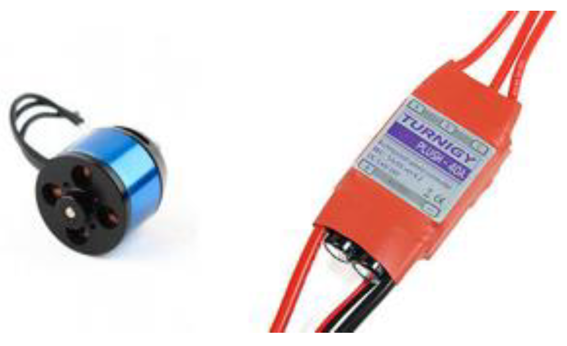
Figure 3.
Motor (left) and speed controller (right).

Figure 4.
Morphing Hub.

Figure 5.
Close-up of the Morphing Hub.

Figure 6.
General power distribution of the quadcopter.

Figure 7.
Quadcopter in (a) normal configuration and (b) quadcopter transitioning from normal to morphed configuration.
Figure 7.
Quadcopter in (a) normal configuration and (b) quadcopter transitioning from normal to morphed configuration.

Figure 8.
Simulation response of (a) roll (l) and (b) pitch (r) attitude between normal and morphed geometries.
Figure 8.
Simulation response of (a) roll (l) and (b) pitch (r) attitude between normal and morphed geometries.

Figure 9.
Trend of changing damping ratio, with changes in the morphing angle.

Figure 10.
Illustrations of the flight paths as described in Table 6.
Figure 10.
Illustrations of the flight paths as described in Table 6.

Figure 11.
Body axis pitch rate, during morphing at Hover conditions.

Figure 12.
Body axis pitch rate, during morphing at Hover conditions—zoomed in.

Figure 13.
Body axis roll rate, during morphing in hover conditions.

Figure 14.
Body axis roll rate during morphing in Hover conditions—zoomed in.

Figure 15.
Body axis yaw rate during morphing in hover conditions.

Figure 16.
Body axis roll rate during morphing at Hover conditions—zoomed in.

Figure 17.
Comparison of pitch rate of Figure-8 flights of the quadcopter in an inclined plane.

Figure 18.
Comparison of pitch rate of Figure-8 flights of the quadcopter in an inclined plane—zoomed in.
Figure 18.
Comparison of pitch rate of Figure-8 flights of the quadcopter in an inclined plane—zoomed in.

Figure 19.
Comparison of roll rate of Figure-8 flights of the quadcopter in an inclined plane.

Figure 20.
Comparison of roll rate of Figure-8 flights of the quadcopter in an inclined plane—zoomed in.
Figure 20.
Comparison of roll rate of Figure-8 flights of the quadcopter in an inclined plane—zoomed in.

Figure 21.
Comparison of yaw rate of Figure-8 flights of the quadcopter in an inclined plane.

Figure 22.
Comparison of yaw rate of Figure-8 flights of the quadcopter in an inclined plane—zoomed in.
Figure 22.
Comparison of yaw rate of Figure-8 flights of the quadcopter in an inclined plane—zoomed in.

Figure 23.
Desired and actual flight path of quadcopter—morphing flights in a horizontal plane.

Figure 24.
Desired and actual flight path of quadcopter—morphing flights in a single inclined plane.
Figure 24.
Desired and actual flight path of quadcopter—morphing flights in a single inclined plane.

Figure 25.
Desired and actual flight path of—morphing flights in a Double Inclined plane.

Figure 26.
Step 1: “sliced pie” trajectory based on 20 waypoints.

Figure 27.
Step 2: “left lobe” trajectory split.

Figure 28.
Step 2: “right lobe” trajectory split.

Figure 29.
A complete “sliced pie” split of the flight path of the UAS, into segments between waypoints.
Figure 29.
A complete “sliced pie” split of the flight path of the UAS, into segments between waypoints.

Figure 30.
Triangle ABC with point P within.

Figure 31.
Triangle ABC with point P outside.

Figure 32.
Calculation of position error between waypoints.


Table 1.
Specifications of the Pixhawk flight controller.
| Component | Description |
|---|---|
| CPU | 168 MHz Cortex-M4F |
| IMU | Invensense MPU6000; 3-axis gyroscope, 3-axis accelerometer, three 16-bit analog-to-digital converters (ADCs) for gyroscope and accelerometer outputs. User-programmable gyroscope full-scale range of ±250, ±500, ±1000, and ±2000°/s and accelerometer full-scale range of ±2 g, ±4 g, ±8 g, and ±16g. |
| Barometer | MEAS MS5611 |
| I/O | 14 PWM Servo outputs |
| Extra connectivity | UART, I2C, GPS |
| Flight log | Pluggable microSD card |
| Firmware Version | ArduPilot, 3.4.1 |
Table 2.
Specifications of brushless DC motor and ESC.
| Motor | ESC | ||
|---|---|---|---|
| Model | KDA 20–22 L | Model | Plush 18 A |
| Kv | 924 | Burst Current | 22 A |
| Operating Current | 6–14 A | Constant Current | 18 A |
| Max. Voltage | 11 v | BEC | 5 v/2 A; Linear, 2–4 cells |
| Size/Weight | 28 × 32 mm; 56 g | Size/Weight | 24 × 45 × 11 mm/19 g |
Table 3.
Specifications of the BEC driving the morphing servo.
 | i. Input Voltage: 5–25 volts |
| ii. Selectable Output: 4.8–9.0 volts | |
| iii. Mode: Switching | |
| iv. LiPo Cells: 2–6 | |
| v. Size/Weight: 30 × 15 × 10 mm/11 g |
Table 4.
Physical, inertial, and geometric properties of the quadcopter used in simulation.
| Parameter | Value | Parameter | Value |
|---|---|---|---|
| , , | |||
| , , | |||
| , , | |||
| mass | 2.324 kg | ||
| arm length | 0.305 m | ||
| 0.0207 k | 0.0137(); 0.0123() k | ||
| 0.0207 k | 0.0276(); 0.0029 () k | ||
| 0.0138 k | 0.0138(); 0.0138() k | ||
| −0.0027(); −0.0043() k |
Table 5.
Step response of roll and pitch attitude in simulation.
| Roll Dynamics | Pitch Dynamics | |||||||
|---|---|---|---|---|---|---|---|---|
| 5.8744 | 0.7310 | 0.5105 | 1.7783 | 5.5352 | 0.7984 | 0.5132 | 1.6368 | |
| 14.8066 | 0.2667 | 0.7089 | 6.7685 | 8.7098 | 0.4630 | 0.5636 | 3.0997 | |
| 15.3960 | 0.2563 | 0.7296 | 7.2485 | 11.6535 | 0.3410 | 0.57 | 4.2566 | |
Table 6.
Flight test parameters.
| Flight Conditions | Parameters |
|---|---|
| “Figure-8” flight path | Horizontal, inclined and double inclined plane |
| Morphing Angle | , , |
| Number of waypoints | 20, 30 (over the entire path) |
| Waypoints with morphed Geometry | No. 4–No. 7 (20), No. 5–No. 11 (30) |
| Velocity | , |
Table 7.
General setup for flight test evaluation of morphed geometry quadcopter configurations.
|
Table 8.
Mean value and standard deviation of body axis angular rates during hover tests.
| Roll | Pitch | Yaw | Roll | Pitch | Yaw | |
|---|---|---|---|---|---|---|
| −0.10162 | 0.149712 | 0.082135 | 3.754336 | 2.70556 | 1.154787 | |
| 0.052661 | 0.120368 | 0.066851 | 5.426002 (44.52%) | 4.567562 (68.82%) | 6.195452 (436.5%) | |
| 0.071171 | 0.20745 | 0.079197 | 6.281651 (67.31%) | 5.24529 (93.87%) | 6.702127 (480.7%) | |
Table 9.
Standard deviation of angular rates of different flights (flights in a horizontal plane).
| v = 1.5 m/s; Waypoints = 20 | v = 2.5 m/s; Waypoints = 20 | |||||
|---|---|---|---|---|---|---|
| 5.7103 | 13.2743 | 23.5161 | 16.3689 | 17.0616 | 26.6821 | |
| 10.4814(83.6%) | 15.597(17.5%) | 22.7085(−3.43%) | 23.3277(42.51%) | 19.3982(13.7%) | 25.7222(−3.6%) | |
| 10.0744(76.4%) | 13.1465(−0.96%) | 24.2962(3.31%) | 17.7324(8.33%) | 18.4482(8.13%) | 27.2056(1.96%) | |
Table 10.
Standard deviation of angular rates of different flights (flights in a single inclined plane).
Table 10.
Standard deviation of angular rates of different flights (flights in a single inclined plane).
| v = 1.5 m/s; Waypoints = 20 | v = 2.5 m/s; Waypoints = 20 | |||||
|---|---|---|---|---|---|---|
| 6.5744 | 11.4717 | 23.529 | 14.8538 | 15.7843 | 27.2415 | |
| 10.6581(62.11%) | 14.6114(27.36%) | 22.7722(−3.21%) | 21.3364(43.64%) | 17.2458(9.25%) | 26.7324(−1.86%) | |
| 9.9941(52%) | 11.7458(2.39%) | 24.3338(3.42%) | 17.6113(18.56%) | 16.8861(7%) | 26.9048(−1.23%) | |
Table 11.
Standard deviation of axis angular rates of different flights (flights in a double inclined plane).
Table 11.
Standard deviation of axis angular rates of different flights (flights in a double inclined plane).
| v = 1.5 m/s; Waypoints = 20 | v = 2.5 m/s; Waypoints = 20 | |||||
|---|---|---|---|---|---|---|
| 6.4357 | 13.2678 | 23.4045 | 16.8838 | 16.9342 | 27.0096 | |
| 11.0187(71.21%) | 14.4729(9%) | 21.3538(−8.76%) | 22.7902(35%) | 16.0106(−5.45%) | 28.1622(4.26%) | |
| 10.3847(61.36%) | 11.8751(−10.5%) | 24.7663(5.81%) | 19.7108(16.74%) | 17.4828(3.23%) | 28.4287(5.25%) | |
Table 12.
Standard deviation of angular rates of different flights (flights in a horizontal plane).
| v = 1.5 m/s; Waypoints = 30 | v = 2.5 m/s; Waypoints = 30 | |||||
|---|---|---|---|---|---|---|
| 7.6676 | 14.2476 | 21.0887 | 14.5061 | 18.2174 | 23.121 | |
| 12.3884(61.56%) | 16.255(14%) | 20.2024(−4.2%) | 17.7009(22%) | 20.703(13.64%) | 24.4376(5.69%) | |
| 10.1845(32.82%) | 13.6735(−4%) | 20.8213(−1.27%) | 17.7756(22.54%) | 19.7693(8.52%) | 24.1675(4.52%) | |
Table 13.
Standard deviation of angular rates of different flights (flights in a single inclined plane).
Table 13.
Standard deviation of angular rates of different flights (flights in a single inclined plane).
| v = 1.5 m/s; Waypoints = 30 | v = 2.5 m/s; Waypoints = 30 | |||||
|---|---|---|---|---|---|---|
| 7.6265 | 13.9759 | 20.6477 | 13.7688 | 18.331 | 22.5695 | |
| 10.6458(39.6%) | 16.2405(16.2%) | 20.9114(1.28%) | 17.0046(23.5%) | 19.3913(5.8%) | 23.4673(4%) | |
| 12.698(66.5%) | 15.9637(14.22%) | 21.7133(5.16%) | 18.1519(31.8%) | 19.7393(7.68%) | 23.782(5.37%) | |
Table 14.
Standard deviation of angular rates of different flights (flights in a double inclined plane).
Table 14.
Standard deviation of angular rates of different flights (flights in a double inclined plane).
| v = 1.5 m/s; Waypoints = 30 | v = 2.5 m/s; Waypoints = 30 | |||||
|---|---|---|---|---|---|---|
| 7.2602 | 13.5614 | 20.4416 | 14.3061 | 17.6015 | 22.2279 | |
| 10.2385(41%) | 15.5668(15.19%) | 21.3065(4.38%) | 16.1706(13%) | 19.8128(12.56%) | 23.3341(5%) | |
| 11.5224(58.7%) | 14.8339(9.76%) | 21.3371(4.53%) | 17.1404(19.81%) | 19.3309(9.82%) | 23.4543(5.5%) | |
Table 15.
Broad description of the “sliced pie” method to identify flight segments.
|
Table 16.
Performance of the UAS in tracking the desired trajectory—normal and morphed geometries.
| Position Accuracy (m) | |||||
|---|---|---|---|---|---|
| Velocity | # of Waypoints | Figure-8 Path | Angle of Morphing | ||
| 1.5 m/s | 20 | Horizontal | 0.147747 | 0.164417 (11.28%) | 0.191469 (29.59%) |
| Inclined Plane | 0.158586 | 0.179997 (13.50%) | 0.173187 (9.21%) | ||
| Double Inclined Plane | 0.174257 | 0.159785 (−8.31%) | 0.181728 (4.29%) | ||
| 30 | Horizontal | 0.159395 | 0.162365 (1.86%) | 0.196734 (23.43%) | |
| Inclined Plane | 0.170629 | 0.165754 (−2.86%) | 0.192818 (13.00%) | ||
| Double Inclined Plane | 0.156425 | 0.17115 (9.41%) | 0.188438 (20.47%) | ||
| 2.5 m/s | 20 | Horizontal | 0.326446 | 0.296922 (−9.04%) | 0.320985 (−1.67%) |
| Inclined Plane | 0.285876 | 0.299318 (4.70%) | 0.328326 (14.85%) | ||
| Double Inclined Plane | 0.299329 | 0.279802 (−6.52%) | 0.313557 (4.75%) | ||
| 30 | Horizontal | 0.300823 | 0.318122 (5.75%) | 0.279573 (−7.06%) | |
| Inclined Plane | 0.301102 | 0.307059 (1.98%) | 0.298945 (−0.72%) | ||
| Double Inclined Plane | 0.284698 | 0.281298 (−1.19%) | 0.267317 (−6.11%) | ||
© 2019 by the authors. Licensee MDPI, Basel, Switzerland. This article is an open access article distributed under the terms and conditions of the Creative Commons Attribution (CC BY) license (http://creativecommons.org/licenses/by/4.0/).
Share and Cite
MDPI and ACS Style
Bai, Y.; Gururajan, S. Evaluation of a Baseline Controller for Autonomous “Figure-8” Flights of a Morphing Geometry Quadcopter: Flight Performance. Drones 2019, 3, 70. https://doi.org/10.3390/drones3030070
AMA Style
Bai Y, Gururajan S. Evaluation of a Baseline Controller for Autonomous “Figure-8” Flights of a Morphing Geometry Quadcopter: Flight Performance. Drones. 2019; 3(3):70. https://doi.org/10.3390/drones3030070
Chicago/Turabian StyleBai, Ye, and Srikanth Gururajan. 2019. "Evaluation of a Baseline Controller for Autonomous “Figure-8” Flights of a Morphing Geometry Quadcopter: Flight Performance" Drones 3, no. 3: 70. https://doi.org/10.3390/drones3030070