Numerical Study of Fractional Order Burgers’-Huxley Equation Using Modified Cubic Splines Approximation

Abstract

This paper aims to explore the numerical solution of non-linear fractional-order Burgers’-Huxley equation based on Caputo’s formulation of fractional derivatives. The equation serves as a versatile tool for analyzing a wide range of physical, biological, and engineering systems, facilitating valuable insights into nonlinear dynamic phenomena. The fractional operator provides a comprehensive mathematical framework that effectively captures the non-locality, hereditary characteristics, and memory effects of various complex systems. The approximation of temporal differential operator is carried out through finite difference based L1 scheme, while spatial discretization is performed using modified cubic B-spline basis functions. The stability as well as convergence analysis of the approach are also presented. Additionally, some numerical test experiments are conducted to evaluate the computational efficiency of a modified fourth-order cubic B-spline (M43BS) approach. Finally, the results presented in the form of tables and graphs highlight the applicability and robustness of M43BS technique in solving fractional-order differential equations. The proposed methodology is preferred for its flexible nature, high accuracy, ease of implementation and the fact that it does not require unnecessary integration of weight functions, unlike other numerical methods such as Galerkin and spectral methods.

1. Introduction

Fractional-order derivatives have gained significant importance in real-world phenomenon due to their greater degree of flexibility in mathematical modeling as well as their ability to represent the inherited characteristics of several objects. Fractional-order operators are non-local in nature, whereas classical differential operators have local characteristics. A number of physical aspects can be effectively modeled through the use of fractional-order integrals and derivative theory. The importance of fractional calculus can be analyzed through the mathematical modeling of numerous rigorous phenomenon, e.g., rotational fluid flow [1], seepage occurring in porous medium [2], viscoelastic properties of polyethylene foams [3], forecasting of national economic growth [4], etc.

Classical PDEs are able to simulate various complex phenomena arising in the fields of fluid mechanics and biology and in many other areas of science and engineering. Non-linear convection–diffusion equations hold significant importance in the study of the propagation of nonlinear dispersive waves and traveling wave forms such as tidal oscillations, surface water waves in shallow rivers, and tsunami waves in a variety of disciplines including oceanography, hydrodynamics, acoustics, and marine engineering. Different researchers are working on developing efficient techniques to obtain analytical as well as numerical solutions for a variety of fractional-order models.

The generalized Burgers’-Huxley equation is one of the significant non-linear partial differential equations (PDEs) illustrating the relationships among reaction procedure, diffusion transports and convection outcomes [5]. Furthermore, this equation also plays a crucial role in different domains such as biology, chemistry, engineering, mathematics, and so on. The model was originally brought into practice by Huxley [6] and was later successfully developed by Burgers [7] as a model to study the turbulent motion of fluids. Classical-order derivatives describe the behaviour of the dependent variable only at integer positions and do not provide any information regarding the behaviour between integer positions. Time fractional PDEs are derived from classical PDEs by substituting a fractional-order derivative in place of the temporal derivative. By including the fractional derivative term in classical PDEs, certain memory characteristics are incorporated into the system. The 1-D generalized non-linear fractional PDE is of the following form [8]:

$$\begin{array}{c}{\phantom{,}}^C{\mathfrak{D}}_{\tau }^{\alpha }\left(W\right)=v_1{\nabla }^{2}W-{\beta }_1{W}^{p_1}\nabla W+{\gamma }_{1}W(1-W^{p_1})(W^{p_1}-\eta )+\mathtt{Z}(\xi ,\tau ),\xi \in [L_{\xi },R_{\xi }],\tau \in [{\tau }_0,T]\hfill \end{array}$$

(1)

subject to following initial and boundary conditions:

$$\begin{array}{c}W(\xi ,{\tau }_0)=ϵ\left(\xi \right),\hfill \end{array}$$

(2)

$$\begin{array}{c}\mathfrak{G}W(\xi ,\tau )=\mathfrak{g}(\xi ,\tau ).\hfill \end{array}$$

(3)

By gathering source and convective terms into a general non-linear term, the above equation can be written as

$$\begin{array}{c}{\phantom{,}}^C{\mathfrak{D}}_{\tau }^{\alpha }\left(W\right)=v_1{\nabla }^{2}W-{\beta }_1{W}^{p_1}\nabla W+\mathfrak{F}(\xi ,\tau ,W),\hfill \end{array}$$

(4)

where $\alpha$ denotes the order of fractional derivative, ${\beta }_1\ge 0$ is a real constant (coefficient of advection term), ${\gamma }_1>0$ (reaction coefficient), $v_1$ is the coefficient of diffusivity, ∇ represents the gradient operator, $p_1\ge 1$ and $\eta \in (0, 1)$ are real constants, $ϵ$ and $\mathfrak{g}$ are known functions, $\mathfrak{G}$ is the boundary operator, $\mathtt{Z}(\xi ,\tau )$ is the source term, and $\mathfrak{F}(\xi ,\tau ,W)={\gamma }_{1}W(1-W^{p_1})(W^{p_1}-\eta )+\mathtt{Z}(\xi ,\tau )$. By setting ${\beta }_1=0$, $\alpha =1$, $v_1=1$, Equation (1) reduces to the generalized Burgers’-Huxley equation illustrating relationships among reaction procedure, diffusion transports, and convection terms [5]:

$${\displaystyle \frac{\partial W}{\partial \tau }}={\nabla }^{2}W-{\beta }_1{W}^{p_1}\nabla W+{\gamma }_{1}W(1-W^{p_1})(W^{p_1}-\eta )+\mathtt{Z}(\xi ,\tau ).$$

(5)

By choosing ${\gamma }_1=0$, Equation (1) is transformed into a generalized fractional Burgers’ Equation (6) which describes many complex problems arising in the field of applied sciences, for instance, the propagation of waves in non-linear dissipative processes, ionic propagation in plasma, solid state physics, etc., [9]:

$${\phantom{,}}^C{\mathfrak{D}}_{\tau }^{\alpha }\left(W\right)=v_1{\nabla }^{2}W-{\beta }_1{W}^{p_1}\nabla W+\mathtt{Z}(\xi ,\tau ).$$

(6)

For ${\beta }_1$ = 0, Equation (1) becomes a generalized fractional Huxley Equation (7), which explains wall motion inside liquid crystals as well as the mechanism of nerve pulse propagation [10]:

$${\phantom{,}}^C{\mathfrak{D}}_{\tau }^{\alpha }\left(W\right)=v_1{\nabla }^{2}W+{\gamma }_{1}W(1-W^{p_1})(W^{p_1}-\eta )+\mathtt{Z}(\xi ,\tau ).$$

(7)

At $p_1=1$, ${\beta }_1,v_1,{\gamma }_1\ne 0$, Equation (1) assumes the form of time fractional Burgers’-Huxley equation (TFBHE), which can be written as

$${\phantom{,}}^C{\mathfrak{D}}_{\tau }^{\alpha }\left(W\right)=v_1{\nabla }^{2}W-{\beta }_{1}W\nabla W+{\gamma }_{1}W(1-W)(W-\eta )+\mathtt{Z}(\xi ,\tau ).$$

(8)

Many definitions of fractional-order operators such as the Riemann–Liouville operator, Caputo’s definition, the Caputo–Fabrizio differential operator, the Atangana–Baleanu fractional operator, etc., have been proposed in the last few decades. Some preliminaries of fractional-order calculus are discussed here in order to understand the subsequent work.

(i) For $\alpha >0$, the Riemann–Liouville fractional integral of order $\alpha$ defined on usual Lebesgue space $L_1[L_{\xi },R_{\xi }]$ by [11] is as follows:

$$\begin{array}{cc}& {\mathfrak{J}}^{\alpha }\left(f\left(\xi \right)\right)={\displaystyle \frac{1}{\Gamma \left(\alpha \right)}}{\int }_{L_{\xi }}^{\xi }{(\xi -s)}^{\alpha -1}f\left(s\right)ds,\hfill \\ \hfill & {\mathfrak{J}}^0\left(f\left(\xi \right)\right)=f\left(\xi \right).\hfill \end{array}$$

For f∈$L_1[L_{\xi },R_{\xi }]$, $\alpha$, $\chi$$\ge 0$ and $\beta >-1$, above operator has following properties:

$$\begin{array}{cc}& {\mathfrak{J}}^{\alpha }{\mathfrak{J}}^{\chi }\left(f\left(\xi \right)\right)={\mathfrak{J}}^{\alpha +\chi }\left(f\left(\xi \right)\right),\hfill \\ \hfill & {\mathfrak{J}}^{\alpha }{\mathfrak{J}}^{\chi }\left(f\left(\xi \right)\right)={\mathfrak{J}}^{\chi }{\mathfrak{J}}^{\alpha }\left(f\left(\xi \right)\right),\hfill \\ \hfill & {\mathfrak{J}}^{\alpha }\left({\xi }^{\beta }\right)={\displaystyle \frac{\Gamma (\beta +1)}{\Gamma (\alpha +\beta +1)}}{(\xi -L_{\xi })}^{\alpha +\beta }.\hfill \end{array}$$

(ii) The fractional-order derivative in terms of the Riemann–Liouville interpretation is [12]

$${\phantom{,}}^{RL}{D}^{\alpha }\left(f\left(\xi \right)\right)={\displaystyle \frac{1}{\Gamma (p-\alpha )}}{\displaystyle \frac{d^p}{d{x}^p}}{\int }_{L_{\xi }}^{\xi }{(\xi -s)}^{p-\alpha -1}f\left(s\right)ds,$$

(9)

for $\xi >0$ and $p-1$<$\alpha$≤p, $p\in {\mathbb{Z}}^{+}$.

(iii) Caputo [12,13] proposed the definition of fractional operator as

$${\phantom{,}}^C{D}^{\alpha }\left(f\left(\xi \right)\right)={\displaystyle \frac{1}{\Gamma (p-\alpha )}}{\int }_{L_{\xi }}^{\xi }{(\xi -s)}^{p-\alpha -1}{f}^p\left(s\right)ds,$$

(10)

where $\alpha \ge 0$ and p = $\lceil \alpha \rceil$. Then,

$$\begin{array}{cc}& {\phantom{,}}^C{D}^{\alpha }{J}^{\alpha }\left(f\left(\xi \right)\right)=f\left(\xi \right),\hfill \\ & J^{\alpha }\left[{\phantom{,}}^C{D}^{\alpha }\left(f\left(\xi \right)\right)\right]=f\left(\xi \right)-\sum _{v=0}^{p-1}{f}^v\left(0^{+}\right){\displaystyle \frac{{(\xi -L_{\xi })}^v}{v!}},\xi >0.\hfill \end{array}$$

(iv) For p to be smallest integer that exceeds $\alpha$, Caputo’s interpretation of the time-fractional derivative of the function $W(\xi ,\tau )$ of order $\alpha$ is defined as follows [12,14]:

$${\phantom{,}}^C{\mathfrak{D}}_{\tau }^{\alpha }\left(W(\xi ,\tau )\right)=\left\{\begin{array}{c}{\displaystyle \frac{1}{\Gamma (1-\alpha )}}{\int }_0^{\tau }{(\tau -y)}^{p-\alpha -1}{\displaystyle \frac{{\partial }^{p}W(\xi ,y)}{\partial y^p}}dy,p-1<\alpha <p\hfill \\ {\displaystyle \frac{{\partial }^{p}W(\xi ,\tau )}{\partial {\tau }^p}},\alpha =p\in \mathbb{N}.\hfill \end{array}\right.$$

(11)

(v) For $W(\xi ,\tau )$ be the function of space ${\mathbb{H}}^1$(0,1), the Caputo–Fabrizio definition of fractional-order differentiation can be represented as [15]

$${\phantom{,}}^{CF}{\mathfrak{D}}_{\tau }^{\alpha }\left(W(\xi ,\tau )\right)={\displaystyle \frac{C\left(\alpha \right)}{1-\alpha }}{\int }_0^{\tau }{\displaystyle \frac{\partial W(\xi ,y)}{\partial y}}exp\left[{\displaystyle \frac{-\alpha }{1-\alpha }}(\tau -y)\right]dy,0<\alpha \le 1,$$

(12)

where C($\alpha$) is a normalization function that satisfies a property as C(0)=C(1)=1.

(vi) Atangana and Baleanu [16] introduced a novel definition based on the non-local and non-singular Mittag–Leffler kernel. For $W(\xi ,\tau )$∈${\mathbb{H}}^1$(0,1), the Atangana–Baleanu operator of order $\alpha$∈$(0, 1]$ in the Riemann–Liouville sense can be expressed as follows:

$${\phantom{,}}^{ABR}{\mathfrak{D}}_{\tau }^{\alpha }\left(W(\xi ,\tau )\right)={\displaystyle \frac{C\left(\alpha \right)}{1-\alpha }}\times {\displaystyle \frac{d}{d\tau }}{\int }_0^{\tau }W(\xi ,y)\times {\mathtt{E}}_{\alpha }\left[{\displaystyle \frac{-\alpha }{1-\alpha }}{(\tau -y)}^{\alpha }\right]dy.$$

(13)

In the case of Caputo, the above differential operator can be formulated as

$${\phantom{,}}^{ABC}{\mathfrak{D}}_{\tau }^{\alpha }\left(W(\xi ,\tau )\right)={\displaystyle \frac{C\left(\alpha \right)}{1-\alpha }}{\int }_0^{\tau }{\displaystyle \frac{\partial W(\xi ,y)}{\partial y}}{\mathtt{E}}_{\alpha }\left[{\displaystyle \frac{-\alpha }{1-\alpha }}{(\tau -y)}^{\alpha }\right]dy,0<\alpha \le 1$$

(14)

where C($\alpha$) denotes the normalization function and ${\mathtt{E}}_{\alpha }$(z)=${\mathtt{E}}_{\alpha ,1}$(z) represents the Mittag–Leffler function defined by [12]:

$${\mathtt{E}}_{\alpha }\left(z\right)=\sum _{i=0}^{\infty }{\displaystyle \frac{z^i}{\Gamma (\alpha i+1)}}$$

where $\Gamma$ denotes the Euler Gamma function, $\alpha$$>0$ and z∈$\mathbb{C}$. Furthermore, the two-parameter Mittag–Leffler function is defined by [12]

$${\mathtt{E}}_{\alpha ,b}\left(z\right)=\sum _{i=0}^{\infty }{\displaystyle \frac{z^i}{\Gamma (\alpha i+b)}},$$

where $\alpha$$>0$, z∈$\mathbb{C}$ and $b\in \mathbb{R}$.

In the literature, several models based on fractional PDEs have been solved by a variety of analytical and numerical methods. An implicit compact operator-based approximation is implemented in [17] for numerical solution of time-dependent Burgers’-Huxley equation. Inc et al. [18] studied a generalized Burgers’-Huxley model involving Riemann–Liouville formulation of the time-fractional derivative by utilizing lie symmetry analysis and a power series expansion approach. A residual power series approach is constructed in [8] by combining Taylor’s series formula with residual error function for solving time-fractional Burgers’-Huxley model. Inc et al. [19] investigated the solution of fractional Burgers’-Huxley equation using a combination method of line- and group-preserving schemes. In this study, the time-fractional derivative is defined by utilizing Caputo’s interpretation for derivatives.

Kumar and Pandey [20] approximated the solution for spatial and temporal fractional-order Burgers’-Huxley models using the Atangana–Baleanu operator in the Caputo sense. The Legendre spectral method is applied for approximating space derivatives, while the temporal-order derivative is discretized via a finite difference scheme. In [21], the existence of bifurcation of fractional Burgers’-Huxley models is examined for various situations of parameter $\delta$ utilizing the residual powers series technique. Tripathi [22] proposed an efficient fractional sub-equation approach in order to find three different types of analytical solutions for $2-D$ nonlinear space–time fractional-order Burgers’-Huxley model. This study includes Jumarie’s modified Riemann–Liouville formulation for defining derivatives in spatial and temporal directions. Furthermore, a Fibonacci polynomials-based collocation approach is introduced in [23] in order to solve variable order Burgers’-Huxley equations having fractional derivatives in spatial as well as temporal directions.

Mazeed et al. [24] presented a collocation technique based on cubic polynomial splines for solving time fractional Burgers’-Huxley model. In this study, time derivatives are handled through a finite difference approach, while discretization of spatial derivatives is achieved using cubic B-splines as basis functions. For 1-D fractional Burgers’-Huxley models, Kanth et al. [25] employed a natural transform decomposition procedure in which the fractional derivative was considered in terms of the Caputo, Caputo–Fabrizio, and Atangana–Baleanu senses. Yang and Liu [26] carried out numerical study of fractional Burgers’-Huxley equations by utilizing a finite difference approach for time-fractional derivatives, and spatial direction was approximated by fourth-order compact approximation. A collocation technique based on extended cubic B-splines is proposed in [27] for the numerical solution of the time-fractional Burgers’-Huxley equations. In this study, a $\theta$-weighted scheme is employed to approximate the temporal domain, while extended cubic splines are utilized to interpolate the derivatives along spatial direction. Furthermore, the stability as well as consistency of the approach are investigated.

Habiba et al. [28] developed an improved Bernoulli sub-equation function approach for solving the generalized fractional-order Burgers’-Huxley equation by incorporating the definition of the conformable fractional derivative. Arifeen et al. [29] implemented the Galerkin approximation to obtain the numerical solution of the fractional Burgers’-Huxley equation, in which the fractional operator is interpreted in terms of the Caputo sense. The study [30] applied iterative approximations and energy estimates to explore the dynamic behaviour of the fractional stochastic Burgers’-Huxley equation under the influence of Levy noise and Brownian motion. Abali and Konuralp [31] investigated the solution of Fredholm–Volterra fractional integro-differential equations utilizing a novel computational method based on shifted Gegenbauer wavelets. A matrix-based collocation approach is proposed in [32] to compute the solution of second-order nonlinear ODEs governed by mixed boundary conditions. Khan et al. [33] derived the numerical solution of parabolic differential equations subject to integral boundary conditions by employing the Haar wavelet-based collocation technique.

The present study provides a numerical solution to a Burgers’-Huxley model incorporating fractional derivative in temporal direction by using a B-spline-based collocation technique in combination with a finite-difference approach. The B-spline is a piecewise polynomial function that inherits smoothness conditions. One distinguishing feature of B-splines is that the resultant matrix for the discretized set of equations is sparse in nature due to its ability to deal with local occurrences. Furthermore, the method constructed by B-splines-based functions does not require any transformation to reduce non-linear differential equation into a simpler form, and as a result, numerical effort is reduced significantly. In order to attain optimal order of convergence along the spatial direction, the current study pertains to some posteriori changes in the second-order derivative of the cubic spline interpolant, leading to the formation of a modified technique.

The organization of the manuscript is as follows: Section 2 is devoted to construction of a modified cubic polynomial basis by adding an extra term to Taylor’s series expansion for the second derivative. Implementation of the suggested technique in the proposed model, which has a fractional derivative in the temporal direction, is presented in Section 3. Study of the stability and convergence criteria is included in Section 4 and Section 5, respectively. To prove the efficacy and applicability of the M43BS approach, five problems based on a fractional-order Burgers’-Huxley model are solved in Section 6. The last section consists of overall conclusions.

2. Construction of Proposed Approach

For a non-linear generalized temporal fractional order Burgers’-Huxley equation incorporating Caputo’s interpretation for derivatives, a numerical approach is proposed in this section. The properties as well as later improvements to the cubic spline interpolating polynomial are provided below:

2.1. Cubic B-Spline Functions

A piecewise polynomial spline exhibits a high degree of smoothness at locations where polynomial parts come together. Consider M as a positive integer and discretize the spatial interval [$L_{\xi },R_{\xi }$] further into M equidistant sub-intervals with each knot point satisfying $L_{\xi }={\xi }_0<{\xi }_1<\dots <{\xi }_{M-1}<{\xi }_M=R_{\xi }$ such that h denotes a step length of fixed size along the spatial direction. According to [34], cubic splines’ basis functions can be expressed as follows:

$${\phi }_l\left(\xi \right)={\displaystyle \frac{1}{h^3}}\left\{\begin{array}{cc}{(\xi -{\xi }_{l-2})}^3,\hfill & \xi \in [{\xi }_{l-2},{\xi }_{l-1}]\hfill \\ h^3+3h^2(\xi -{\xi }_{l-1})+3h{(\xi -{\xi }_{l-1})}^2-3{(\xi -{\xi }_{l-1})}^3,\hfill & \xi \in [{\xi }_{l-1},{\xi }_l]\hfill \\ h^3+3h^2({\xi }_{l+1}-\xi )+3h{({\xi }_{l+1}-\xi )}^2-3{({\xi }_{l+1}-\xi )}^3,\hfill & \xi \in [{\xi }_l,{\xi }_{l+1}]\hfill \\ {({\xi }_{l+2}-\xi )}^3,\hfill & \xi \in [{\xi }_{l+1},{\xi }_{l+2}]\hfill \\ 0,\hfill & Otherwise,\hfill \end{array}\right.$$

where the linearly independent set of functions $\{{\phi }_{-1},{\phi }_0,{\phi }_1,\dots ,{\phi }_{M-1},{\phi }_M,{\phi }_{M+1}\}$ forms the basis of a finite dimensional subspace of ${\mathbb{C}}^2[L_{\xi },R_{\xi }]$ with dimension ($M+3$) over the interval $[L_{\xi },R_{\xi }]$. Each cubic B-spline includes four domain elements and four spline functions occupying each finite element $[{\xi }_l,{\xi }_{l+1}]$. So, four additional knot points are needed outside the domain $[L_{\xi },R_{\xi }]$, and these points are positioned as ${\xi }_{-2}<{\xi }_{-1}<{\xi }_0$ and ${\xi }_M<{\xi }_{M+1}<{\xi }_{M+2}$. The expansion of approximate solution $u(\xi ,\tau )$ in terms of cubic spline basis functions is as follows:

$$u(\xi ,\tau )=\sum _{l=-1}^{M+1}{\delta }_l\left(\tau \right){\phi }_l\left(\xi \right),$$

(15)

where the basis functions for proposed approximation ${\phi }_l\left(\xi \right)$, for $l=-1,0,\dots ,M+1$ and ${\delta }_{-1}\left(\tau \right)$, ${\delta }_0\left(\tau \right)$, ${\delta }_1\left(\tau \right),\dots$, ${\delta }_{M+1}\left(\tau \right)$ are unknown coefficients that depend upon time. These coefficients must be computed from initial as well as boundary conditions. The first- and second-order derivatives of the numerical solution $u(\xi ,\tau )$ at the knots ${\xi }_l$ are associated the with time-dependent parameters listed below:

$$\begin{array}{cc}& u({\xi }_l,\tau )={\delta }_{l-1}\left(\tau \right)+4{\delta }_l\left(\tau \right)+{\delta }_{l+1}\left(\tau \right),l=0,1,\dots ,M,\hfill \\ \hfill & u_{\xi }({\xi }_l,\tau )={\displaystyle \frac{-3}{h}}\left({\delta }_{l-1}\left(\tau \right)-{\delta }_{l+1}\left(\tau \right)\right),\hfill \\ \hfill & u_{\xi \xi }({\xi }_l,\tau )={\displaystyle \frac{6}{h^2}}\left({\delta }_{l-1}\left(\tau \right)-2{\delta }_l\left(\tau \right)+{\delta }_{l+1}\left(\tau \right)\right).\hfill \end{array}$$

(16)

2.2. Construction of Modified Cubic B-Splines

Assume that the below-mentioned conditions are satisfied by cubic interpolating polynomials for the function at different knots:

(I)

the approximation condition, in the case of $l=0,1,\dots ,M$:

$$u({\xi }_l,\tau )=W({\xi }_l,\tau ),$$

(17)

(II)

Third point at end knot points, i.e., for $l=0$ and M:

$$u_{\xi \xi }({\xi }_l,\tau )=W_{\xi \xi }({\xi }_l,\tau )-{\displaystyle \frac{h^2}{12}}{W}_{\xi \xi \xi \xi }({\xi }_l,\tau ).$$

(18)

Theorem 1.

Below provided results are true for unique cubic interpolating function $u(\xi ,\tau )$ corresponding to $W(\xi ,\tau )$, where $W(\xi ,\tau )$ is a sufficiently smooth function on interval $[L_{\xi },R_{\xi }]$ and satisfies Equations (17) and (18):

$$u_{\xi }({\xi }_l,\tau )=W_{\xi }({\xi }_l,\tau )+O\left(h^4\right),$$

(19)

$$u_{\xi \xi }({\xi }_l,\tau )=W_{\xi \xi }({\xi }_l,\tau )-{\displaystyle \frac{h^2}{12}}{W}_{\xi \xi \xi \xi }({\xi }_l,\tau )+O\left(h^4\right).$$

(20)

Furthermore,

$$\left|\right|W^{\left(\mathtt{m}\right)}-u^{\left(\mathtt{m}\right)}{\left|\right|}_{\infty }=O\left(h^{4-\mathtt{m}}\right),\mathtt{m}=0,1,2.$$

(21)

where $W^{\left(\mathtt{m}\right)}$ and $u^{\left(\mathtt{m}\right)}$ denote $m^{th}$-order derivatives with respect to ‘ξ’.

Proof. 

It is already available in [35,36]. □

Lemma 1.

If $W(\xi ,\tau )$∈${\mathbb{C}}^6[L_{\xi },R_{\xi }]$, then the below-listed relations are valid for higher-order derivatives of exact solutions having equally spaced partitions across different knot points:

$$\begin{array}{cc}\hfill & W_{\xi \xi \xi \xi }({\xi }_0,\tau )={\displaystyle \frac{2u_{\xi \xi }({\xi }_0,\tau )-5u_{\xi \xi }({\xi }_1,\tau )+4u_{\xi \xi }({\xi }_2,\tau )-u_{\xi \xi }({\xi }_3,\tau )}{h^2}}+O\left(h^2\right),\hfill \\ \hfill \\ \hfill & W_{\xi \xi \xi \xi }({\xi }_l,\tau )={\displaystyle \frac{u_{\xi \xi }({\xi }_{l-1},\tau )-2u_{\xi \xi }({\xi }_l,\tau )+u_{\xi \xi }({\xi }_{l+1},\tau )}{h^2}}+O\left(h^2\right),l=1\left(1\right)M-1,\hfill \\ \hfill \\ \hfill & W_{\xi \xi \xi \xi }({\xi }_M,\tau )={\displaystyle \frac{2u_{\xi \xi }({\xi }_M,\tau )-5u_{\xi \xi }({\xi }_{M-1},\tau )+4u_{\xi \xi }({\xi }_{M-2},\tau )-u_{\xi \xi }({\xi }_{M-3},\tau )}{h^2}}+O\left(h^2\right).\hfill \end{array}$$

Proof. 

By using Taylor’s series expansion and finite differences, the above relations are proved in [35]. □

Corollary 1.

If $\mathcal{W}(\xi ,\tau )$∈${\mathbb{C}}^6[L_{\xi },R_{\xi }]$, then the expressions shown hereunder are satisfied at various knot points:

$$\begin{array}{cc}\hfill & W_{\xi }({\xi }_l,\tau )=u_{\xi }({\xi }_l,\tau )+O\left(h^4\right),l=0\left(1\right)M,\hfill \\ \hfill \\ \hfill & W_{\xi \xi }({\xi }_0,\tau )={\displaystyle \frac{14u_{\xi \xi }({\xi }_0,\tau )-5u_{\xi \xi }({\xi }_1,\tau )+4u_{\xi \xi }({\xi }_2,\tau )-u_{\xi \xi }({\xi }_3,\tau )}{12}}+O\left(h^4\right),\hfill \\ \hfill \\ \hfill & W_{\xi \xi }({\xi }_l,\tau )={\displaystyle \frac{u_{\xi \xi }({\xi }_{l-1},\tau )+10u_{\xi \xi }({\xi }_l,\tau )+u_{\xi \xi }({\xi }_{l+1},\tau )}{12}}+O\left(h^4\right),l=1\left(1\right)M-1,\hfill \\ \hfill \\ \hfill & W_{\xi \xi }({\xi }_M,\tau )={\displaystyle \frac{14u_{\xi \xi }({\xi }_M,\tau )-5u_{\xi \xi }({\xi }_{M-1},\tau )+4u_{\xi \xi }({\xi }_{M-2},\tau )-u_{\xi \xi }({\xi }_{M-3},\tau )}{12}}+O\left(h^4\right).\hfill \end{array}$$

Proof. 

Available in [35]. □

3. Implementation of the Proposed Method

In order to discretize the fractional order derivative in temporal direction, this section presents the finite difference approximation. Assume step size in time for some positive integer N defined by $d\tau ={\displaystyle \frac{T}{N}}$ with time instant ${\tau }_k={\tau }_0+kd\tau$, for $k=0,1,\dots ,N$ respectively. By using Caputo’s formulation of derivative for ${\phantom{,}}^C{\mathfrak{D}}_{\tau }^{\alpha }\left(W\right)$, an approximation of the temporal fractional-order derivative defined in Equation (11) at time $\tau ={\tau }_{k+1}$ is as follows [37]:

$$\begin{array}{cc}\hfill {\phantom{,}}^C{\mathfrak{D}}_{\tau }^{\alpha }\left(W(\xi ,{\tau }^{k+1})\right)=& {\displaystyle \frac{1}{\Gamma (1-\alpha )}}{\int }_0^{{\tau }_{k+1}}{({\tau }_{k+1}-y)}^{-\alpha }{\displaystyle \frac{\partial W(\xi ,y)}{\partial y}}dy,\hfill \\ \hfill =& {\displaystyle \frac{1}{\Gamma (1-\alpha )}}\sum _{\varphi =0}^k{\int }_{{\tau }_{\varphi }}^{{\tau }_{\varphi +1}}{({\tau }_{k+1}-y)}^{-\alpha }{\displaystyle \frac{\partial W(\xi ,y)}{\partial y}}dy,\hfill \\ \hfill =& {\displaystyle \frac{1}{\Gamma (1-\alpha )}}\sum _{\varphi =0}^k{\displaystyle \frac{W(\xi ,{\tau }_{\varphi +1})-W(\xi ,{\tau }_{\varphi })}{d\tau }}{\int }_{{\tau }_{\varphi }}^{{\tau }_{\varphi +1}}{({\tau }_{k+1}-y)}^{-\alpha }dy+e_{d\tau }^{k+1},\hfill \\ \hfill =& {\displaystyle \frac{1}{\Gamma (1-\alpha )}}\sum _{\varphi =0}^k{\displaystyle \frac{W(\xi ,{\tau }_{\varphi +1})-W(\xi ,{\tau }_{\varphi })}{d\tau }}{\int }_{{\tau }_{k-\varphi }}^{{\tau }_{k+1-\varphi }}{\displaystyle \frac{d\omega }{{\omega }^{\alpha }}}+e_{d\tau }^{k+1}.\hfill \end{array}$$

Further simplification gives [38]

$${\phantom{,}}^C{\mathfrak{D}}_{\tau }^{\alpha }\left(W(\xi ,{\tau }^{k+1})\right)=\left\{\begin{array}{c}\begin{array}{cc}\gamma \sum _{\varphi =0}^k{\lambda }_{\varphi }\left(W^{k-\varphi +1}-W^{k-\varphi }\right)+O\left({\left(d\tau \right)}^{2-\alpha }\right),\hfill & \hfill 0<\alpha <1\\ {\displaystyle \frac{W(\xi ,{\tau }_{k+1})-W(\xi ,{\tau }_k)}{d\tau }}+O\left(d\tau \right),\hfill & \hfill \alpha =1,\end{array}\hfill \end{array}\right.$$

(22)

where $\gamma ={\left(d\tau \right)}^{-\alpha }/\Gamma (2-\alpha )$, ${\lambda }_{\varphi }={(\varphi +1)}^{1-\alpha }-{\left(\varphi \right)}^{1-\alpha }$ and $\omega =({\tau }_{k+1}-y)$. The coefficients ${\lambda }_{\varphi }$’s satisfy the following properties:

$$\left\{\begin{array}{c}{\lambda }_0=1,\hfill \\ {\lambda }_0>{\lambda }_1>{\lambda }_2\dots >{\lambda }_i,{\lambda }_{\varphi }\to 0when\varphi \to \infty ,\hfill \\ {\lambda }_{\varphi }>0incase\varphi =0,1,2,\dots ,k,\hfill \\ {\sum }_{\varphi =0}^k({\lambda }_{\varphi }-{\lambda }_{\varphi +1})+{\lambda }_{k+1}=(1-{\lambda }_1)+{\sum }_{\varphi =1}^{k-1}({\lambda }_{\varphi }-{\lambda }_{\varphi +1})+{\lambda }_k=1.\hfill \end{array}\right.$$

Integrating Equation (1) by employing backward rectangular rule for the left-hand side and the source term and utilizing trapezoidal rule for the remaining terms together with Equation (22) yields:

$$\begin{array}{cc}& \gamma \sum _{\varphi =0}^k{\lambda }_{\varphi }\left(W^{k-\varphi +1}-W^{k-\varphi }\right)-v_1\left[{\displaystyle \frac{{\left(W_{\xi \xi }\right)}^{k+1}+{\left(W_{\xi \xi }\right)}^k}{2}}\right]+{\beta }_1\left[{\displaystyle \frac{{\left(W^{p_1}{W}_{\xi }\right)}^{k+1}+{\left(W^{p_1}{W}_{\xi }\right)}^k}{2}}\right]\hfill \\ & -{\displaystyle \frac{{\gamma }_1}{2}}\left[(1+\eta )\left[{\left(W^{p_1+1}\right)}^{k+1}+{\left(W^{p_1+1}\right)}^k\right]-\left[{\left(W^{2p_1+1}\right)}^{k+1}+{\left(W^{2p_1+1}\right)}^k\right]-\eta \left[W^{k+1}+W^k\right]\right]+\mathtt{Z}(\xi ,{\tau }^{k+1}).\hfill \end{array}$$

(23)

Using the following quasi-linearization procedure, the non-linear terms are linearized [39]:

$$\begin{array}{cc}& {\left(W^{p_1+1}\right)}^{k+1}+{\left(W^{p_1+1}\right)}^k=(1-p_1){\left(W^{p_1+1}\right)}^k+(1+p_1){\left(W^{p_1}\right)}^k{W}^{k+1}+O{\left(d\tau \right)}^2\hfill \\ & {\left(W^{p_1}{W}_{\xi }\right)}^{k+1}+{\left(W^{p_1}{W}_{\xi }\right)}^k=(1-p_1){\left(W^{p_1}{W}_{\xi }\right)}^k+{\left(W^{p_1}\right)}^k{\left(W_{\xi }\right)}^{k+1}+p_1{\left(W\right)}^{k+1}{\left({\left(W\right)}^{p_1-1}{W}_{\xi }\right)}^k+O{\left(d\tau \right)}^2\hfill \\ & {\left(W^{2p_1+1}\right)}^{k+1}+{\left(W^{2p_1+1}\right)}^k=(1-2p_1){\left(W^{2p_1+1}\right)}^k+(1+2p_1){\left(W^{2p_1}\right)}^k{W}^{k+1}+O{\left(d\tau \right)}^2.\hfill \end{array}$$

On rearranging the factors at various time levels, the following expression is produced:

$$\begin{array}{cc}& \left[\left({\displaystyle \frac{p_1{\beta }_1}{2}}{\left(W^{p_1-1}{W}_{\xi }\right)}^k\right)-{\displaystyle \frac{{\gamma }_1}{2}}\left((1+\eta )(1+p_1){\left(W^{p_1}\right)}^k-(1+2p_1){\left(W^{2p_1}\right)}^k-\eta \right)+\gamma \right]W^{k+1}\hfill \\ & +\left[{\displaystyle \frac{{\beta }_1}{2}}{\left(W^{p_1}\right)}^k\right]W_{\xi }^{k+1}-\left[{\displaystyle \frac{v_1}{2}}\right]W_{\xi \xi }^{k+1}=\gamma \sum _{\varphi =0}^{k-1}\left({\lambda }_{\varphi }-{\lambda }_{\varphi +1}\right)W^{k-\varphi }+\gamma {\lambda }_k{W}^0+{\displaystyle \frac{{\beta }_1}{2}}\left[(p_1-1){\left(W^{p_1}{W}_{\xi }\right)}^k\right]\hfill \\ & +{\displaystyle \frac{{\gamma }_1}{2}}\left[(1+\eta )(1-p_1){\left(W^{p_1+1}\right)}^k-(1-2p_1){\left(W^{2p_1+1}\right)}^k-\eta {\left(W\right)}^k\right]+\left[{\displaystyle \frac{v_1}{2}}\right]W_{\xi \xi }^k+\mathtt{Z}(\xi ,{\tau }^{k+1}).\hfill \end{array}$$

(24)

At any $l^{th}$ knot point, the resultant equation is

$$P_l{\left(W\right)}_l^{k+1}+Q_l{\left(W_{\xi }\right)}_l^{k+1}+R_l{\left(W_{\xi \xi }\right)}_l^{k+1}={\mathtt{T}}_l,$$

(25)

where

$$\begin{array}{cc}& P_l=\left[\left({\displaystyle \frac{p_1{\beta }_1}{2}}{\left(W_l^{p_1-1}\right)}^k{\left(W_{\xi }\right)}_l^k\right)-{\displaystyle \frac{{\gamma }_1}{2}}\left((1+\eta )(1+p_1){\left(W_l^{p_1}\right)}^k-(1+2p_1){\left(W_l^{2p_1}\right)}^k-\eta \right)+\gamma \right],\hfill \\ & Q_l={\displaystyle \frac{{\beta }_1}{2}}{\left(W_l^{p_1}\right)}^k,R_l=-{\displaystyle \frac{v_1}{2}},\hfill \\ & {\mathtt{T}}_l=\gamma \sum _{\varphi =0}^{k-1}\left({\lambda }_{\varphi }-{\lambda }_{\varphi +1}\right)W_l^{k-\varphi }+\gamma {\lambda }_k{W}_l^0+{\displaystyle \frac{{\beta }_1}{2}}\left[(p_1-1)\left(W_l^{p_1}\right){\left(W_{\xi }\right)}_l^k\right]\hfill \\ & +{\displaystyle \frac{{\gamma }_1}{2}}\left[(1+\eta )(1-p_1){\left(W_l^{p_1+1}\right)}^k-(1-2p_1){\left(W_l^{2p_1+1}\right)}^k-\eta {\left(W\right)}_l^k\right]+\left[{\displaystyle \frac{v_1}{2}}\right]{\left(W_{\xi \xi }\right)}_l^k+\mathtt{Z}({\xi }_l,{\tau }^{k+1}).\hfill \end{array}$$

(26)

On substituting the computed values for function $W(\xi ,\tau )$ along with its derivatives of higher order at the specified knots and by clubbing the coefficients of time-dependent parameters ${\delta }_l^{k+1}$, the corresponding equations are formed as follows:

For $l=0:$

$$\begin{array}{cc}& \left(P_0-{\displaystyle \frac{3Q_0}{h}}+{\displaystyle \frac{7R_0}{h^2}}\right){\delta }_{-1}^{k+1}+\left(4P_0-{\displaystyle \frac{33R_0}{2h^2}}\right){\delta }_0^{k+1}+\left(P_0+{\displaystyle \frac{3Q_0}{h}}+{\displaystyle \frac{14R_0}{h^2}}\right){\delta }_1^{k+1}-{\displaystyle \frac{7R_0}{h^2}}{\delta }_2^{k+1}+{\displaystyle \frac{3R_0}{h^2}}{\delta }_3^{k+1}\hfill \\ & -{\displaystyle \frac{R_0}{2h^2}}{\delta }_4^{k+1}={\mathtt{T}}_0+O(h^4+d{\tau }^{2-\alpha }),\hfill \end{array}$$

$${\mathtt{b}}_0{\delta }_{-1}^{k+1}+{\mathtt{c}}_0{\delta }_0^{k+1}+{\mathtt{d}}_0{\delta }_1^{k+1}+{\mathtt{e}}_0{\delta }_2^{k+1}+{\mathtt{f}}_0{\delta }_3^{k+1}+{\mathtt{g}}_0{\delta }_4^{k+1}={\mathtt{T}}_0+O(h^4+d{\tau }^{2-\alpha }),$$

(27)

where

$$\begin{array}{cc}& {\mathtt{b}}_0=\left(P_0-{\displaystyle \frac{3Q_0}{h}}+{\displaystyle \frac{7R_0}{h^2}}\right),{\mathtt{c}}_0=\left(4P_0-{\displaystyle \frac{33R_0}{2h^2}}\right),{\mathtt{d}}_0=\left(P_0+{\displaystyle \frac{3Q_0}{h}}+{\displaystyle \frac{14R_0}{h^2}}\right),\hfill \\ & {\mathtt{e}}_0=-{\displaystyle \frac{7R_0}{h^2}},{\mathtt{f}}_0={\displaystyle \frac{3R_0}{h^2}},{\mathtt{g}}_0=-{\displaystyle \frac{R_0}{2h^2}}.\hfill \end{array}$$

For $l=1,2,\dots ,M-1$:

$$\begin{array}{cc}& {\displaystyle \frac{R_l}{2h^2}}{\delta }_{l-2}^{k+1}+\left(P_l-{\displaystyle \frac{3Q_l}{h}}+{\displaystyle \frac{4R_l}{h^2}}\right){\delta }_{l-1}^{k+1}+\left(4P_l-{\displaystyle \frac{9R_l}{h^2}}\right){\delta }_l^{k+1}+\left(P_l+{\displaystyle \frac{3Q_l}{h}}+{\displaystyle \frac{4R_l}{h^2}}\right){\delta }_{l+1}^{k+1}+{\displaystyle \frac{R_l}{2h^2}}{\delta }_{l+2}^{k+1}\hfill \\ & ={\mathtt{T}}_l+O(h^4+d{\tau }^{2-\alpha }),\hfill \end{array}$$

$$\kappa {\delta }_{l-2}^{k+1}+{\mathtt{c}}_l{\delta }_{l-1}^{k+1}+{\mathtt{d}}_l{\delta }_l^{k+1}+{\mathtt{e}}_l{\delta }_{l+1}^{k+1}+\kappa {\delta }_{l+2}^{k+1}={\mathtt{T}}_l+O(h^4+d{\tau }^{2-\alpha }),$$

(28)

where

$$\kappa ={\displaystyle \frac{R_l}{2h^2}},{\mathtt{c}}_l=\left(P_l-{\displaystyle \frac{3Q_l}{h}}+{\displaystyle \frac{4R_l}{h^2}}\right),{\mathtt{d}}_l=\left(4P_l-{\displaystyle \frac{9R_l}{h^2}}\right),{\mathtt{e}}_l=\left(P_l+{\displaystyle \frac{3Q_l}{h}}+{\displaystyle \frac{4R_l}{h^2}}\right).$$

For $l=M:$

$$\begin{array}{cc}& -{\displaystyle \frac{R_M}{2h^2}}{\delta }_{M-4}^{k+1}+{\displaystyle \frac{3R_M}{h^2}}{\delta }_{M-3}^{k+1}-{\displaystyle \frac{7R_M}{h^2}}{\delta }_{M-2}^{k+1}+\left(P_M-{\displaystyle \frac{3Q_M}{h}}+{\displaystyle \frac{14R_M}{h^2}}\right){\delta }_{M-1}^{k+1}+\left(4P_M-{\displaystyle \frac{33R_M}{2h^2}}\right){\delta }_M^{k+1}\hfill \\ & +\left(P_M+{\displaystyle \frac{3Q_M}{h}}+{\displaystyle \frac{7R_M}{h^2}}\right){\delta }_{M+1}^{k+1}={\mathtt{T}}_M+O(h^4+d{\tau }^{2-\alpha }),\hfill \end{array}$$

$${\mathtt{b}}_M{\delta }_{M-4}^{k+1}+{\mathtt{c}}_M{\delta }_{M-3}^{k+1}+{\mathtt{d}}_M{\delta }_{M-2}^{k+1}+{\mathtt{e}}_M{\delta }_{M-1}^{k+1}+{\mathtt{f}}_M{\delta }_M^{k+1}+{\mathtt{g}}_M{\delta }_{M+1}^{k+1}={\mathtt{T}}_M+O(h^4+d{\tau }^{2-\alpha }),$$

(29)

where

$$\begin{array}{cc}& {\mathtt{b}}_M=-{\displaystyle \frac{R_M}{2h^2}},{\mathtt{c}}_M={\displaystyle \frac{3R_M}{h^2}},{\mathtt{d}}_M=-{\displaystyle \frac{7R_M}{h^2}},{\mathtt{e}}_M=\left(P_M-{\displaystyle \frac{3Q_M}{h}}+{\displaystyle \frac{14R_M}{h^2}}\right),\hfill \\ & {\mathtt{f}}_M=\left(4P_M-{\displaystyle \frac{33R_M}{2h^2}}\right),{\mathtt{g}}_M=\left(P_M+{\displaystyle \frac{3Q_M}{h}}+{\displaystyle \frac{7R_M}{h^2}}\right).\hfill \end{array}$$

In addition to the above, two more equations are derived using boundary conditions as

$${\delta }_{-1}^{k+1}+4{\delta }_0^{k+1}+{\delta }_1^{k+1}={\mathfrak{g}}_1\left(\right(k+1\left)d\tau \right),$$

and

$${\delta }_{M-1}^{k+1}+4{\delta }_M^{k+1}+{\delta }_{M+1}^{k+1}={\mathfrak{g}}_2((k+1)d\tau ).$$

The matrix-form representation of the equations mentioned above is as follows:

$$\mathfrak{K}\mathfrak{Z}=\mathfrak{T}$$

where ${\mathfrak{Z}}_{i,1}={\left[{\delta }_{i-2}^{k+1}\right]}_{i=1}^{M+3}$ and

$${\mathfrak{T}}_{i,1}=\left\{\begin{array}{cc}{\mathfrak{g}}_1\left(\right(k+1\left)d\tau \right),\hfill & i=1,\hfill \\ {\mathfrak{T}}_{i-2},\hfill & 2\le i\le M+2,\hfill \\ {\mathfrak{g}}_2\left(\right(k+1\left)d\tau \right),\hfill & i=M+3.\hfill \end{array}\right.$$

In matrix $\mathfrak{K},$ the first three elements of the first row and last three elements of the last row are (1,4,1), while the first six elements of the second row and final six elements of the second-to-last row are $({\mathtt{b}}_0,{\mathtt{c}}_0,{\mathtt{d}}_0,{\mathtt{e}}_0,{\mathtt{f}}_0,{\mathtt{g}}_0)$ and $({\mathtt{b}}_M,{\mathtt{c}}_M,{\mathtt{d}}_M,{\mathtt{e}}_M,{\mathtt{f}}_M,{\mathtt{g}}_M)$, respectively. The remaining entries of the matrix are listed below:

$${\left[\mathfrak{A}\right]}_{i=3,j=1}^{M+1,M+3}=\left\{\begin{array}{cc}\kappa ,\hfill & |i-j|=2\hfill \\ {\mathtt{c}}_{i-2},\hfill & i-j=1\hfill \\ {\mathtt{d}}_{i-2},\hfill & i=j\hfill \\ {\mathtt{e}}_{i-2},\hfill & j-i=1\hfill \\ 0,\hfill & otherwise.\hfill \end{array}\right.$$

The final system of equations attained is utilized for ${[{\delta }_{-1}^{k+1},{\delta }_0^{k+1},{\delta }_1^{k+1},\dots ,{\delta }_{M-1}^{k+1},{\delta }_M^{k+1},{\delta }_{M+1}^{k+1}]}^T.$ By using this vector in Equation (15), the required numerical solution at the ${(k+1)}^{th}$ temporal level for $k=0,1,2,\dots ,N$ is obtained.

Initial Vector

In order to initiate the iterative procedure, the initial vector ${[{\delta }_{-1}^0,{\delta }_0^0,{\delta }_1^0,\dots ,{\delta }_{M-1}^0,{\delta }_M^0,{\delta }_{M+1}^0]}^T$ needs to be specified to determine the solution for the succeeding temporal levels. For this, an initial condition is used at each knot point, i.e., $W({\xi }_l,{\tau }_0)$=$ϵ\left({\xi }_l\right)$. As a result, a system of ($M+1$) equations containing ($M+3$) unknowns will be obtained. To find a unique solution for this system, two additional conditions are employed, i.e., $W_{\xi }({\xi }_0,{\tau }_0)$=${ϵ}_{\xi }\left({\xi }_0\right)$ and $W_{\xi }({\xi }_M,{\tau }_0)$=${ϵ}_{\xi }\left({\xi }_M\right)$. Finally, the system of equations will result into a matrix of order $(M+3)$×$(M+3)$ that can be represented as follows:

$$\begin{array}{c}\hfill \mathfrak{A}{\delta }^0=\mathfrak{D}.\end{array}$$

In matrix $\mathfrak{A},$ the first three elements of the first row and last three elements of last row are (${\displaystyle \frac{-3}{h}}$,0,${\displaystyle \frac{3}{h}}$). Remaining entries of the matrix are shown below:

$${\left[\mathfrak{A}\right]}_{i=3,j=1}^{M+1,M+3}=\left\{\begin{array}{cc}1,\hfill & |i-j|=1\hfill \\ 4,\hfill & i=j\hfill \\ 0,\hfill & otherwise.\hfill \end{array}\right.$$

Here, ${\delta }^0$ denotes a column vector of order $(M+3)$×1 and $\mathfrak{D}={[{ϵ}_{\xi }\left({\xi }_0\right),ϵ\left({\xi }_0\right),\dots ,{ϵ}_{\xi }\left({\xi }_M\right)]}^T$. The above system will be solved in order to determine the values of unknown time-dependent coefficients’ ${\delta }_l^{\prime }$s at the initial time level. In this study, Matlab R2021a software has been utilized for performing numerical computations.

4. Stability Analysis

In order to determine the stability of the M43BS technique, the von Neumann approach is used. First, linearize the non-linear terms by assuming $m_1$=max $W^{p_1}$, and upon further employing the Crank–Nicolson approach in Equation (1), the following expression is obtained:

$$\begin{array}{cc}& \gamma \sum _{\varphi =0}^k{\lambda }_{\varphi }\left(W_l^{k-\varphi +1}-W_l^{k-\varphi }\right)=v_1\left[{\displaystyle \frac{{\left(W_{\xi \xi }\right)}_l^{k+1}+{\left(W_{\xi \xi }\right)}_l^k}{2}}\right]-{\beta }_1{m}_1\left[{\displaystyle \frac{{\left(W_{\xi }\right)}_l^{k+1}+{\left(W_{\xi }\right)}_l^k}{2}}\right]\hfill \\ & +{\gamma }_1(1-m_1)(m_1-\eta )\left[{\displaystyle \frac{W_l^{k+1}+W_l^k}{2}}\right]+\mathtt{Z}({\xi }_l,{\tau }^{k+1}).\hfill \end{array}$$

(30)

On separating the terms at various time levels and assuming ${\gamma }_1(1-m_1)(m_1-\eta )=m_2$, the above equation reduces to

$$\begin{array}{cc}& \left[\gamma -{\displaystyle \frac{m_2}{2}}\right]{\left(W\right)}_l^{k+1}+{\displaystyle \frac{m_1{\beta }_1}{2}}{\left(W_{\xi }\right)}_l^{k+1}-{\displaystyle \frac{v_1}{2}}{\left(W_{\xi \xi }\right)}_l^{k+1}\hfill \\ & =\left[{\displaystyle \frac{m_2}{2}}\right]{\left(W\right)}_l^k+{\displaystyle \frac{v_1}{2}}{\left(W_{\xi \xi }\right)}_l^k-{\displaystyle \frac{m_1{\beta }_1}{2}}{\left(W_{\xi }\right)}_l^k+\gamma \sum _{\varphi =0}^{k-1}\left({\lambda }_{\varphi }-{\lambda }_{\varphi +1}\right)W_l^{k-\varphi }+\gamma {\lambda }_k{W}_l^0+\mathtt{Z}({\xi }_l,{\tau }^{k+1}).\hfill \end{array}$$

Further, the above equation can be written as

$$\begin{array}{cc}\hfill & a_1{\left(W\right)}_l^{k+1}+a_2{\left(W_{\xi }\right)}_l^{k+1}-a_3{\left(W_{\xi \xi }\right)}_l^{k+1}=a_4{\left(W\right)}_l^k-a_2{\left(W_{\xi }\right)}_l^k+a_3{\left(W_{\xi \xi }\right)}_l^k+\hfill \\ & \gamma \sum _{\varphi =0}^{k-1}\left({\lambda }_{\varphi }-{\lambda }_{\varphi +1}\right)W_l^{k-\varphi }+\gamma {\lambda }_k{W}_l^0+\mathtt{Z}({\xi }_l,{\tau }^{k+1}),\hfill \end{array}$$

(31)

where $a_1=\gamma -{\displaystyle \frac{m_2}{2}},a_2={\displaystyle \frac{m_1{\beta }_1}{2}},$$a_3={\displaystyle \frac{v_1}{2}},a_4={\displaystyle \frac{m_2}{2}}$. By substituting the approximate solution and its higher-order derivatives, the resulting expression is

$$\begin{array}{cc}& a_1({\delta }_{l-1}^{k+1}+4{\delta }_l^{k+1}+{\delta }_{l+1}^{k+1})+{\displaystyle \frac{3a_2}{h}}({\delta }_{l+1}^{k+1}-{\delta }_{l-1}^{k+1})-{\displaystyle \frac{a_3}{2h^2}}({\delta }_{l-2}^{k+1}+8{\delta }_{l-1}^{k+1}-18{\delta }_l^{k+1}+8{\delta }_{l+1}^{k+1}+{\delta }_{l+2}^{k+1})\hfill \\ & =\mathtt{Z}({\xi }_l,{\tau }^{k+1})+a_4({\delta }_{l-1}^k+4{\delta }_l^k+{\delta }_{l+1}^k)+{\displaystyle \frac{a_3}{2h^2}}({\delta }_{l-2}^k+8{\delta }_{l-1}^k-18{\delta }_l^k+8{\delta }_{l+1}^k+{\delta }_{l+2}^k)-{\displaystyle \frac{3a_2}{h}}({\delta }_{l+1}^k-{\delta }_{l-1}^k)\hfill \\ & +\gamma \sum _{\varphi =0}^{k-1}\left({\lambda }_{\varphi }-{\lambda }_{\varphi +1}\right)\left({\delta }_{l-1}^{k-\varphi }+4{\delta }_l^{k-\varphi }+{\delta }_{l+1}^{k-\varphi }\right)+\gamma {\lambda }_k\left({\delta }_{l-1}^0+4{\delta }_l^0+{\delta }_{l+1}^0\right).\hfill \end{array}$$

(32)

After simplification, Equation (32) takes the form

$$\begin{array}{cc}& \left(-{\displaystyle \frac{a_3}{2h^2}}\right){\delta }_{l-2}^{k+1}+\left(a_1-{\displaystyle \frac{8a_3}{2h^2}}-{\displaystyle \frac{3a_2}{h}}\right){\delta }_{l-1}^{k+1}+\left(4a_1+{\displaystyle \frac{18a_3}{2h^2}}\right){\delta }_l^{k+1}+\left(a_1+{\displaystyle \frac{3a_2}{h}}-{\displaystyle \frac{8a_3}{2h^2}}\right){\delta }_{l+1}^{k+1}\hfill \\ & -\left({\displaystyle \frac{a_3}{2h^2}}\right){\delta }_{l+2}^{k+1}=\mathtt{Z}({\xi }_l,{\tau }^{k+1})+\left({\displaystyle \frac{a_3}{2h^2}}\right){\delta }_{l-2}^k+\left(a_4+{\displaystyle \frac{8a_3}{2h^2}}+{\displaystyle \frac{3a_2}{h}}\right){\delta }_{l-1}^k+\left(4a_4-{\displaystyle \frac{18a_3}{2h^2}}\right){\delta }_l^k\hfill \\ & +\left(a_4+{\displaystyle \frac{8a_3}{2h^2}}-{\displaystyle \frac{3a_2}{h}}\right){\delta }_{l+1}^k+\left({\displaystyle \frac{a_3}{2h^2}}\right){\delta }_{l+2}^k+\gamma \sum _{\varphi =0}^{k-1}\left({\lambda }_{\varphi }-{\lambda }_{\varphi +1}\right)({\delta }_{l-1}^{k-\varphi }+4{\delta }_l^{l-\varphi }+{\delta }_{l+1}^{k-\varphi })\hfill \\ & +\gamma {\lambda }_k({\delta }_{l-1}^0+4{\delta }_l^0+{\delta }_{l+1}^0).\hfill \end{array}$$

(33)

The above equation can be rewritten as follows:

$$\begin{array}{cc}& z_1{\delta }_{l-2}^{k+1}+z_2{\delta }_{l-1}^{k+1}+z_3{\delta }_l^{k+1}+z_4{\delta }_{l+1}^{k+1}+z_1{\delta }_{l+2}^{k+1}=\mathtt{Z}({\xi }_l,{\tau }^{k+1})-z_1{\delta }_{l-2}^k+z_5{\delta }_{l-1}^k\hfill \\ & +z_6{\delta }_l^k+z_7{\delta }_{l+1}^k-z_1{\delta }_{l+2}^k+\gamma \sum _{\varphi =0}^{k-1}\left({\lambda }_{\varphi }-{\lambda }_{\varphi +1}\right)({\delta }_{l-1}^{k-\varphi }+4{\delta }_l^{k-\varphi }+{\delta }_{l+1}^{k-\varphi })\hfill \\ & +\gamma {\lambda }_k({\delta }_{l-1}^0+4{\delta }_l^0+{\delta }_{l+1}^0),\hfill \end{array}$$

(34)

where

$$\begin{array}{cc}& z_1=-{\displaystyle \frac{a_3}{2h^2}},z_2=a_1-{\displaystyle \frac{8a_3}{2h^2}}-{\displaystyle \frac{3a_2}{h}},z_3=4a_1+{\displaystyle \frac{18a_3}{2h^2}},\hfill \\ & z_4=a_1-{\displaystyle \frac{8a_3}{2h^2}}+{\displaystyle \frac{3a_2}{h}},z_5=a_4+{\displaystyle \frac{8a_3}{2h^2}}+{\displaystyle \frac{3a_2}{h}},z_6=4a_4-{\displaystyle \frac{18a_3}{2h^2}},z_7=a_4+{\displaystyle \frac{8a_3}{2h^2}}-{\displaystyle \frac{3a_2}{h}}.\hfill \end{array}$$

(35)

Upon inserting the solution in single Fourier mode ${\delta }_l^k$=$\mathtt{A}{\rho }^{k}exp\left(\iota l\mathtt{w}h\right)$ in Equation (34), where $\mathtt{A}$ is the size of amplitude, $\mathtt{w}$ denotes mode number, h represents spatial step length and $\iota$=$\sqrt{-1}$, following equation is formed:

$$\begin{array}{cc}& z_1{\rho }^{k+1}{e}^{\iota (l-2)\mathtt{w}h}+z_2{\rho }^{k+1}{e}^{\iota (l-1)\mathtt{w}h}+z_3{\rho }^{k+1}{e}^{\iota l\mathtt{w}h}+z_4{\rho }^{k+1}{e}^{\iota (l+1)\mathtt{w}h}+z_1{\rho }^{k+1}{e}^{\iota (l+2)\mathtt{w}h}=\hfill \\ & -z_1{\rho }^k{e}^{\iota (l-2)\mathtt{w}h}+z_5{\rho }^k{e}^{\iota (l-1)\mathtt{w}h}+z_6{\rho }^k{e}^{\iota l\mathtt{w}h}+z_7{\rho }^k{e}^{\iota (l+1)\mathtt{w}h}-z_1{\rho }^k{e}^{\iota (l+2)\mathtt{w}h}+\hfill \\ & \gamma \sum _{\varphi =0}^{k-1}\left({\lambda }_{\varphi }-{\lambda }_{\varphi +1}\right)({\rho }^{k-\varphi }{e}^{\iota (l-1)\mathtt{w}h}+4{\rho }^{k-\varphi }{e}^{\iota l\mathtt{w}h}+{\rho }^{k-\varphi }{e}^{\iota (l+1)\mathtt{w}h})+\hfill \\ & \gamma {\lambda }_k({\rho }^0{e}^{\iota (l-1)\mathtt{w}h}+4{\rho }^0{e}^{\iota l\mathtt{w}h}+{\rho }^0{e}^{\iota (l+1)\mathtt{w}h})+\mathtt{Z}({\xi }_l,{\tau }^{k+1}).\hfill \end{array}$$

(36)

On simplification, the expression can be written as follows:

$$\begin{array}{cc}\hfill {\rho }^{k+1}& ={\displaystyle \frac{{\rho }^k\left[-2z_{1}cos\left(2\mathtt{w}h\right)+(z_5+z_7)cos\left(\mathtt{w}h\right)+\iota (z_7-z_5)sin\left(\mathtt{w}h\right)+z_6\right]}{\left[2z_{1}cos\left(2\mathtt{w}h\right)+(z_2+z_4)cos\left(\mathtt{w}h\right)+\iota (z_4-z_2)sin\left(\mathtt{w}h\right)+z_3\right]}}\hfill \\ & +{\displaystyle \frac{{\displaystyle \gamma \left(2cos\left(\mathtt{w}h\right)+4\right)\left[\sum _{\varphi =0}^{k-1}\left({\lambda }_{\varphi }-{\lambda }_{\varphi +1}\right){\rho }^{k-\varphi }+{\lambda }_k{\rho }^0\right]+\mathtt{Z}({\xi }_l,{\tau }^{k+1})e^{-\iota l\mathtt{w}h}}}{\left[2z_{1}cos\left(2\mathtt{w}h\right)+(z_2+z_4)cos\left(\mathtt{w}h\right)+\iota (z_4-z_2)sin\left(\mathtt{w}h\right)+z_3\right]}}.\hfill \end{array}$$

(37)

After inserting values of $z_i$’s, the above expression becomes

$$\begin{array}{cc}\hfill {\rho }^{k+1}& ={\displaystyle \frac{{\rho }^k\left[\frac{v_1}{2h^2}cos\left(2\mathtt{w}h\right)+(m_2+\frac{4v_1}{h^2})cos\left(\mathtt{w}h\right)+2m_2-\frac{18v_1}{4h^2}-\iota \frac{3m_1{\beta }_1}{h}sin\left(\mathtt{w}h\right)\right]}{-\frac{v_1}{2h^2}cos\left(2\mathtt{w}h\right)+\left(2\gamma -m_2-\frac{4v_1}{h^2}\right)cos\left(\mathtt{w}h\right)+4\gamma -2m_2+\frac{18v_1}{4h^2}+\iota \frac{3m_1{\beta }_1}{h}sin\left(\mathtt{w}h\right)}}\hfill \\ & +{\displaystyle \frac{{\displaystyle \gamma \left(2cos\left(\mathtt{w}h\right)+4\right)\left[\sum _{\varphi =0}^{k-1}\left({\lambda }_{\varphi }-{\lambda }_{\varphi +1}\right){\rho }^{k-\varphi }+{\lambda }_k{\rho }^0\right]+\mathtt{Z}({\xi }_l,{\tau }^{k+1})e^{-\iota l\mathtt{w}h}}}{-\frac{v_1}{2h^2}cos\left(2\mathtt{w}h\right)+\left(2\gamma -m_2-\frac{4v_1}{h^2}\right)cos\left(\mathtt{w}h\right)+4\gamma -2m_2+\frac{18v_1}{4h^2}+\iota \frac{3m_1{\beta }_1}{h}sin\left(\mathtt{w}h\right)}}.\hfill \end{array}$$

(38)

Based on stability criteria, the approach will be stable if the magnitude of ${\rho }^{k+1}$ is less than or equal to one for all k. By employing the principle of mathematical induction, it is observed that $\left|\rho \right|\le 1$ for varying values of parameters, i.e., $\gamma$, $\mathtt{w}$, h, and $\alpha$. This result demonstrates the unconditional stability of the $M43BS$ approach.

5. Convergence Analysis

This section estimates the convergence analysis by utilizing the Marcos method [40]. Consider ${⨿}_{\xi }=\{{\xi }_l;0\le l\le M\}$ and ${⨿}_{\tau }=\{{\tau }_k;0\le k\le N\}$ be evenly spaced division of spatial $[L_{\xi },R_{\xi }]$ and temporal domains $[0,T]$ with step sizes h and $d\tau$, respectively. On defining two vectors $\mathcal{X}$=(${\mathcal{X}}_0$,${\mathcal{X}}_1,\dots$,${\mathcal{X}}_M$) and $\mathcal{Y}$=(${\mathcal{Y}}_0$,${\mathcal{Y}}_1,\dots$,${\mathcal{Y}}_M$) on ${⨿}_{\xi }$, consider difference notation as

$$\begin{array}{cc}\hfill \Delta \mathcal{X}={\mathcal{X}}_{l+1}-{\mathcal{X}}_l,(\mathcal{X},\mathcal{Y})=\sum _{l=0}^{M}h{\mathcal{X}}_l{\mathcal{Y}}_l,& \\ \hfill ({\mathcal{X}}_{\xi \xi },\mathcal{X})=-({\mathcal{X}}_{\xi },{\mathcal{X}}_{\xi }){,\left|\right|\mathcal{X}\left|\right|}^2=(\mathcal{X},\mathcal{X}),& \\ \hfill ({\mathcal{X}}_{\xi \xi },\mathcal{Y})=-({\mathcal{X}}_{\xi },{\mathcal{Y}}_{\xi }),({\mathcal{X}}_{\xi },\mathcal{Y})=-(\mathcal{X},{\mathcal{Y}}_{\xi }).\end{array}$$

(39)

Additionally, take into account the continuity of functions $W_{\tau \tau }$, $W_{\xi \xi \xi \xi }$ over the domains $[L_{\xi },R_{\xi }]$ and $[0,T]$ together with a constant $\mathtt{C}$ independent of h, $d\tau$, l, and k and assume different values at various locations together with smoothness conditions as

$$|W_{\tau \tau }|\le \mathtt{C},|W_{\xi \xi \xi \xi }|\le \mathtt{C},(\xi ,\tau )\in {\ominus }_{\xi }\times {\ominus }_{\tau }.$$

(40)

Lemma 2.

Assume that the sequence of real numbers $\{{\mathfrak{v}}_0,{\mathfrak{v}}_1,\dots ,{\mathfrak{v}}_k,\dots \}$ has the following characteristics: ${\mathfrak{v}}_k$≥0, ${\mathfrak{v}}_k$≤${\mathfrak{v}}_{k-1}$ and ${\mathfrak{v}}_{k+1}+{\mathfrak{v}}_{k-1}\ge 2{\mathfrak{v}}_k$. After that, each vector in a sequence $({\mathbb{Y}}_1,{\mathbb{Y}}_2,\dots ,{\mathbb{Y}}_R)$ with $\mathfrak{R}$ real entries, where $\mathfrak{R}$ is any positive integer, brings forth

$$\sum _{k=0}^{\mathfrak{R}-1}\left(\sum _{r=0}^k{\mathfrak{v}}_r{\mathbb{Y}}_{k+1-r}\right){\mathbb{Y}}_{k+1}\ge 0.$$

(41)

Now, for the proposed method, the obtained expressions are as follows:

$$\begin{array}{cc}& \gamma \sum _{\varphi =0}^k{\lambda }_{\varphi }\left(W_l^{k-\varphi +1}-W_l^{k-\varphi }\right)-{\displaystyle \frac{m_2}{2}}{\left(W\right)}_l^{k+1}+{\displaystyle \frac{m_1{\beta }_1}{2}}{\left(W_{\xi }\right)}_l^{k+1}-{\displaystyle \frac{v_1}{2}}{\left(W_{\xi \xi }\right)}_l^{k+1}\hfill \\ & ={\displaystyle \frac{m_2}{2}}{\left(W\right)}_l^k+{\displaystyle \frac{v_1}{2}}{\left(W_{\xi \xi }\right)}_l^k-{\displaystyle \frac{m_1{\beta }_1}{2}}{\left(W_{\xi }\right)}_l^k+\mathtt{Z}({\xi }_l,{\tau }^{k+1})+O\left(h^4+{\left(d\tau \right)}^{2-\alpha }\right).\hfill \end{array}$$

(42)

and

$$\begin{array}{cc}& \gamma \sum _{\varphi =0}^k{\lambda }_{\varphi }\left(u_l^{k-\varphi +1}-u_l^{k-\varphi }\right)-{\displaystyle \frac{m_2}{2}}{\left(u\right)}_l^{k+1}+{\displaystyle \frac{m_1{\beta }_1}{2}}{\left(u_{\xi }\right)}_l^{k+1}-{\displaystyle \frac{v_1}{2}}{\left(u_{\xi \xi }\right)}_l^{k+1}\hfill \\ & ={\displaystyle \frac{m_2}{2}}{\left(u\right)}_l^k+{\displaystyle \frac{v_1}{2}}{\left(u_{\xi \xi }\right)}_l^k-{\displaystyle \frac{m_1{\beta }_1}{2}}{\left(u_{\xi }\right)}_l^k+\mathtt{Z}({\xi }_l,{\tau }^{k+1}).\hfill \end{array}$$

(43)

Here, the exact and numerical values are denoted by $W(\xi ,\tau )$ and $u(\xi ,\tau )$, respectively.

Theorem 2.

Given that $W(\xi ,\tau )$ and $u(\xi ,\tau )$ are solutions of fractional model (1) and Equation (42), respectively, and that $W(\xi ,\tau )$ satisfies the smoothness criteria (40), then for each $\tau \ge 0$ and sufficiently small h and $d\tau$, the below-mentioned relation holds:

$$\left|\right|E^{k+1}\left|\right|\le O\left(h^4+{\left(d\tau \right)}^{2-\alpha }\right),$$

(44)

where $E_l^{k+1}$= $W({\xi }_l,{\tau }^{k+1})-u({\xi }_l,{\tau }^{k+1})$.

Proof. 

On subtracting Equation (43) from Equation (42), the error equation is obtained as follows:

$$\Theta {\mathfrak{E}}_{\mathfrak{l}}^{k+1}+{\displaystyle \frac{m_1{\beta }_1}{2}}{\left(E_{\xi }\right)}_l^{k+1}-{\displaystyle \frac{v_1}{2}}{\left(E_{\xi \xi }\right)}_l^{k+1}+\gamma \sum _{\varphi =0}^k{\lambda }_{\varphi }\Delta {\mathfrak{E}}_{\mathfrak{l}}^{k-\varphi +1}=-\Theta {\mathfrak{E}}_{\mathfrak{l}}^k-{\displaystyle \frac{m_1{\beta }_1}{2}}{\left(E_{\xi }\right)}_l^k+{\displaystyle \frac{v_1}{2}}{\left(E_{\xi \xi }\right)}_l^k+{\mathfrak{U}}_{\mathfrak{l}}^{k+1},$$

(45)

where $\Theta =-{\displaystyle \frac{m_2}{2}}$, and ${\mathfrak{U}}_l^{k+1}=O\left(h^4+{\left(d\tau \right)}^{2-\alpha }\right)$. After multiplying both sides of Equation (45) by $h{E}_l^{k+1}$ and adding up the terms for l, which range from 0 to M, the following form is assumed:

$$\begin{array}{cc}\hfill \left|\right|E^{k+1}{\left|\right|}^2=& -{\displaystyle \frac{m_1{\beta }_1}{2\Theta }}({\left(E\right)}_{\xi }^{k+1},E^{k+1})+{\displaystyle \frac{v_1}{2\Theta }}({\left(E\right)}_{\xi \xi }^{k+1},E^{k+1})-{\displaystyle \frac{\gamma }{\Theta }}\sum _{\varphi =0}^k{\lambda }_{\varphi }(\Delta E^{k-\varphi +1},E^{k+1})\hfill \\ & -(E^k,E^{k+1})-{\displaystyle \frac{m_1{\beta }_1}{2\Theta }}({\left(E\right)}_{\xi }^k,E^{k+1})+{\displaystyle \frac{v_1}{2\Theta }}({\left(E\right)}_{\xi \xi }^k,E^{k+1})+{\displaystyle \frac{1}{\Theta }}({\mathfrak{U}}^{k+1},E^{k+1}),\hfill \\ \hfill =& -{\displaystyle \frac{m_1{\beta }_1}{2\Theta }}({\left(E\right)}_{\xi }^{k+1},E^{k+1})-{\displaystyle \frac{v_1}{2\Theta }}({\left(E\right)}_{\xi }^{k+1},{\left(E\right)}_{\xi }^{k+1})-{\displaystyle \frac{\gamma }{\Theta }}\sum _{\varphi =0}^k{\lambda }_{\varphi }(\Delta E^{k-\varphi +1},E^{k+1})\hfill \\ & -(E^k,E^{k+1})-{\displaystyle \frac{m_1{\beta }_1}{2\Theta }}({\left(E\right)}_{\xi }^k,E^{k+1})-{\displaystyle \frac{v_1}{2\Theta }}({\left(E\right)}_{\xi }^k,{\left(E\right)}_{\xi }^{k+1})+{\displaystyle \frac{1}{\Theta }}({\mathfrak{U}}^{k+1},E^{k+1}),\hfill \\ \hfill =& -{\displaystyle \frac{m_1{\beta }_1}{2\Theta }}({\left(E\right)}_{\xi }^{k+1},E^{k+1})-{\displaystyle \frac{v_1}{2\Theta }}{\left|\right|\left(E\right)}_{\xi }^{k+1}{\left|\right|}^2-{\displaystyle \frac{\gamma }{\Theta }}\sum _{\varphi =0}^k{\lambda }_{\varphi }(\Delta E^{k-\varphi +1},E^{k+1})\hfill \\ & -(E^k,E^{k+1})-{\displaystyle \frac{m_1{\beta }_1}{2\Theta }}({\left(E\right)}_{\xi }^k,E^{k+1})-{\displaystyle \frac{v_1}{2\Theta }}({\left(E\right)}_{\xi }^k,{\left(E\right)}_{\xi }^{k+1})+{\displaystyle \frac{1}{\Theta }}({\mathfrak{U}}^{k+1},E^{k+1}).\hfill \end{array}$$

After simplifications, the following expression is obtained:

$$\left|\right|E^{k+1}{\left|\right|}^2+{\displaystyle \frac{\gamma }{\Theta }}\sum _{\varphi =0}^k{\lambda }_{\varphi }(\Delta E^{k-\varphi +1},E^{k+1})\le {\displaystyle \frac{1}{\Theta }}({\mathfrak{U}}^{k+1},E^{k+1}).$$

On writing the terms recursively, we obtain

$$\begin{array}{cc}& \left|\right|E^k{\left|\right|}^2+{\displaystyle \frac{\gamma }{\Theta }}\sum _{\varphi =0}^{k-1}{\lambda }_{\varphi }(\Delta E^{k-\varphi },E^k)\le {\displaystyle \frac{1}{\Theta }}({\mathfrak{U}}^k,E^k),\hfill \\ & \left|\right|E^{k-1}{\left|\right|}^2+{\displaystyle \frac{\gamma }{\Theta }}\sum _{\varphi =0}^{k-2}{\lambda }_{\varphi }(\Delta E^{k-\varphi -1},E^{k-1})\le {\displaystyle \frac{1}{\Theta }}({\mathfrak{U}}^{k-1},E^{k-1})\hfill \\ & ⋮⋮⋮\hfill \\ & \left|\right|E^1{\left|\right|}^2+{\displaystyle \frac{\gamma }{\Theta }}\sum _{\varphi =0}^0{\lambda }_{\varphi }(\Delta E^{1-\varphi },E^1)\le {\displaystyle \frac{1}{\Theta }}({\mathfrak{U}}^1,E^1),\hfill \end{array}$$

and summing up all the above inequalities results in

$$\sum _{\varphi =0}^k\left|\right|E^{k+1}{\left|\right|}^2+{\displaystyle \frac{\gamma }{\Theta }}\sum _{\widehat{m}=0}^k\sum _{\varphi =0}^{\widehat{m}}{\lambda }_{\varphi }(\Delta E^{\widehat{m}-\varphi +1},E^{\widehat{m}+1})\le {\displaystyle \frac{1}{\Theta }}\sum _{\varphi =0}^k({\mathfrak{U}}^{\varphi +1},E^{\varphi +1}).$$

(46)

Using Equation (41), it follows that

$${\displaystyle \frac{\gamma }{\Theta }}\sum _{\widehat{m}=0}^k\sum _{\varphi =0}^{\widehat{m}}{\lambda }_{\varphi }(\Delta E^{\widehat{m}-\varphi +1},E^{\widehat{m}+1})\ge 0,$$

and Equation (46) takes the form

$$\sum _{\varphi =0}^k\left|\right|E^{k+1}{\left|\right|}^2\le {\displaystyle \frac{1}{\Theta }}\sum _{\varphi =0}^k({\mathfrak{U}}^{\varphi +1},E^{\varphi +1}).$$

Therefore,

$$\left|\right|E^{k+1}{\left|\right|}^2\le {\displaystyle \frac{1}{\Theta }}({\mathfrak{U}}^{\varphi +1},E^{\varphi +1}).$$

(47)

On applying the Cauchy–Schwarz inequality

$$<{\mathfrak{s}}_1,{\mathfrak{s}}_2>\le \left|\right|{\mathfrak{s}}_1{\left|\right|}_2\left|\right|{\mathfrak{s}}_2{\left|\right|}_2,$$

Equation (47) results in

$$\left|\right|E^{k+1}{\left|\right|}^2\le {\displaystyle \frac{1}{\Theta }}({\mathfrak{U}}^{\varphi +1},E^{\varphi +1})\le {\displaystyle \frac{1}{\Theta }}\left|\right|{\mathfrak{U}}^{\varphi +1}\left|\right|\left|\right|E^{\varphi +1}\left|\right|,$$

which implies that

$$\left|\right|E^{k+1}{\left|\right|}^2\le {\displaystyle \frac{1}{\Theta }}\left|\right|{\mathfrak{U}}^{k+1}\left|\right|\left|\right|E^{k+1}\left|\right|.$$

Dividing throughout by $\left|\right|E^{k+1}\left|\right|$ yields

$$\left|\right|E^{k+1}\left|\right|\le {\displaystyle \frac{1}{\Theta }}\left|\right|{\mathfrak{U}}^{k+1}\left|\right|.$$

The above inequality gives that

$$\left|\right|E^{k+1}\left|\right|\le O\left(h^4+{\left(d\tau \right)}^{2-\alpha }\right).$$

Thus, fourth-order convergence in a spatial direction is achieved through a modified collocation approach, while for the temporal domain, the order of convergence is $O\left({\left(d\tau \right)}^{2-\alpha }\right)$. Consequently, $O\left(h^4+{\left(d\tau \right)}^{2-\alpha }\right)$ is the order of convergence of the M43BS approach. □

6. Numerical Examples and Discussion

This section focuses on numerical solutions of generalized Burgers’-Huxley equations involving fractional operators. The method’s accuracy has been determined by utilizing Euclidean error norm $L_2$,

$$L_2=\sqrt{h\sum _{l=0}^M{|W({\xi }_l,\tau )-u({\xi }_l,\tau )|}^2},$$

and maximum error norm $L_{\infty }$,

$$L_{\infty }=\underset{0\le l\le M}{max}|W({\xi }_l,\tau )-u({\xi }_l,\tau )|.$$

Here, exact and numerical values at knots ${\xi }_l$, $l=0,1,2,\dots ,M$, are represented by variables $W({\xi }_l,\tau )$ and $u({\xi }_l,\tau )$, respectively.

The order of convergence is calculated using the formula:

$$Order={\displaystyle \frac{log\left(E\left(M_1\right)/E\left(M_2\right)\right)}{log(M_2/M_1)}},$$

where $E\left(M_1\right)$ and $E\left(M_2\right)$ are the errors with $M_1$ and $M_2$ number of divisions along a spatial direction.

Example 1.

Take TFBHE (8) together with the coefficients ${\beta }_1=0.01$, $v_1=1$, ${\gamma }_1=1$ depending upon the initial condition

$$W(\xi ,0)=0,0\le \xi \le 1,$$

as well as the end conditions

$$W(0,\tau )=0,W(1,\tau )=0,\tau \in \left[0,T\right].$$

The source term $\mathtt{Z}(\xi ,\tau )$ is

$$\begin{array}{cc}\hfill \mathtt{Z}(\xi ,\tau )=& (\xi -{\xi }^2){\tau }^{\alpha }{\displaystyle \frac{\Gamma (2\alpha +1)}{\Gamma (1+\alpha )}}+{\beta }_1(\xi -{\xi }^2)(1-2\xi ){\tau }^{4\alpha }+2v_1{\tau }^{2\alpha }\hfill \\ & -{\gamma }_1\left[(\xi -{\xi }^2){\tau }^{2\alpha }\right]\left[1-(\xi -{\xi }^2){\tau }^{2\alpha }\right]\left[(\xi -{\xi }^2){\tau }^{2\alpha }-\eta \right].\hfill \end{array}$$

The exact solution of the problem is given below [24]:

$$W(\xi ,\tau )=(\xi -{\xi }^2){\tau }^{2\alpha }.$$

Using parameters $\alpha =0.5$, $\eta =0.75$, $d\tau =0.00045$, and $M=100$, error norms for Problem 1 are compared to those reported in [24] for various values of temporal levels in

Table 1. Comparison of error norms of Example 1 for different values of T when $0\le \xi \le 1$ and $\alpha =0.5$.

T	$\mathit{M}=100,\mathit{d}\mathit{\tau }=4.5\times {10}^{-4}$				$\mathit{M}=100,\mathit{d}\mathit{\tau }=4.5\times {10}^{-6}$		$\mathit{M}=10,\mathit{d}\mathit{\tau }=2.1\times {10}^{-3}$
	M43BS		[24]		M43BS		M43BS
	${\mathit{L}}_{\mathbf{2}}$	${\mathit{L}}_{\infty }$	${\mathit{L}}_{\mathbf{2}}$	${\mathit{L}}_{\infty }$	${\mathit{L}}_{\mathbf{2}}$	${\mathit{L}}_{\infty }$	${\mathit{L}}_{\mathbf{2}}$	${\mathit{L}}_{\infty }$
1	2.294$\times {10}^{-6}$	3.235$\times {10}^{-6}$	1.620 $\times {10}^{-5}$	1.100$\times {10}^{-4}$	2.294$\times {10}^{-8}$	3.234$\times {10}^{-8}$	1.071$\times {10}^{-5}$	1.511$\times {10}^{-5}$
0.75	2.614$\times {10}^{-6}$	3.685$\times {10}^{-6}$	$5.000\times {10}^{-8}$	3.000$\times {10}^{-7}$	2.613$\times {10}^{-8}$	3.684$\times {10}^{-8}$	1.220$\times {10}^{-5}$	1.721$\times {10}^{-5}$
0.5	3.149$\times {10}^{-6}$	4.438$\times {10}^{-6}$	$4.826\times {10}^{-6}$	3.700$\times {10}^{-5}$	3.148$\times {10}^{-8}$	4.437$\times {10}^{-8}$	1.470$\times {10}^{-5}$	2.072$\times {10}^{-5}$
0.25	4.354$\times {10}^{-6}$	6.134$\times {10}^{-6}$	1.060$\times {10}^{-6}$	1.020$\times {10}^{-5}$	4.351$\times {10}^{-6}$	6.130$\times {10}^{-6}$	2.032$\times {10}^{-5}$	2.863$\times {10}^{-6}$

. The results indicate that the present approach is performing better as compared to the methodology described in [24] for the same problem. For distinct choices of spatial partitions M, the $L_2$ as well as $L_{\infty }$ error norms are presented in

Table 2. Error norms for Example 1 at $T=0.5$ for some values of $\alpha$ when $0\le \xi \le 1$, ${\left(h\right)}_m={\displaystyle \frac{1}{2^{m+1}}}$, and $d\tau =0.01$.

$\mathit{\alpha }$	m	h	${\mathit{L}}_2$	${\mathit{L}}_{\mathit{\infty }}$
	1	0.25	1.491$\times {10}^{-5}$	2.823$\times {10}^{-5}$
	2	0.125	1.551$\times {10}^{-5}$	2.872$\times {10}^{-5}$
0.05	3	0.0625	1.551$\times {10}^{-5}$	2.869$\times {10}^{-5}$
	4	0.03125	1.551$\times {10}^{-5}$	2.869$\times {10}^{-5}$
	5	0.015625	1.551$\times {10}^{-5}$	2.869$\times {10}^{-5}$
	1	0.25	3.950$\times {10}^{-5}$	5.566$\times {10}^{-5}$
	2	0.125	3.950$\times {10}^{-5}$	5.566$\times {10}^{-5}$
0.95	3	0.0625	3.950$\times {10}^{-5}$	5.566$\times {10}^{-5}$
	4	0.03125	3.950$\times {10}^{-5}$	5.566$\times {10}^{-5}$
	5	0.015625	3.950$\times {10}^{-5}$	5.566$\times {10}^{-5}$

, for $d\tau =0.01$, $\eta =0.75$ at temporal scale $T=0.5$. For different values of fractional order $\alpha$ and $M=40,N=40,\eta =0.5$, the absolute error is given in

Table 3. Comparison of absolute error of Example 1 at different values of $\alpha$ when $0\le \xi \le 1$, $N=40$, $M=40$, $\eta =0.5$, and $T=0.1,0.01$.

T	$\mathit{\xi }$	$\mathit{\alpha }=0.1$	$\mathit{\alpha }=0.3$	$\mathit{\alpha }=0.5$	$\mathit{\alpha }=0.7$	$\mathit{\alpha }=0.9$	$\mathit{\alpha }=1$
0.1	0.1	2.861$\times {10}^{-7}$	1.520$\times {10}^{-5}$	1.675$\times {10}^{-5}$	1.433$\times {10}^{-5}$	5.952$\times {10}^{-6}$	7.038$\times {10}^{-11}$
	0.3	2.534$\times {10}^{-5}$	3.982$\times {10}^{-5}$	4.338$\times {10}^{-5}$	3.706$\times {10}^{-5}$	1.533$\times {10}^{-5}$	2.160$\times {10}^{-10}$
	0.5	3.949$\times {10}^{-5}$	4.888$\times {10}^{-5}$	5.334$\times {10}^{-5}$	1.881$\times {10}^{-5}$	5.441$\times {10}^{-5}$	2.855$\times {10}^{-10}$
	0.7	2.535$\times {10}^{-5}$	3.982$\times {10}^{-5}$	4.338$\times {10}^{-5}$	3.707$\times {10}^{-5}$	1.533$\times {10}^{-5}$	2.195$\times {10}^{-10}$
	0.9	2.361$\times {10}^{-7}$	1.520$\times {10}^{-5}$	1.676$\times {10}^{-5}$	1.433$\times {10}^{-5}$	5.952$\times {10}^{-6}$	7.278$\times {10}^{-11}$
0.01	0.1	2.199$\times {10}^{-6}$	7.341$\times {10}^{-6}$	4.246$\times {10}^{-6}$	1.358$\times {10}^{-6}$	1.675$\times {10}^{-7}$	5.954$\times {10}^{-16}$
	0.3	2.033$\times {10}^{-5}$	1.901$\times {10}^{-5}$	1.0960$\times {10}^{-5}$	3.467$\times {10}^{-6}$	4.152$\times {10}^{-7}$	2.646$\times {10}^{-15}$
	0.5	2.864$\times {10}^{-5}$	2.338$\times {10}^{-5}$	1.345$\times {10}^{-5}$	4.234$\times {10}^{-6}$	5.007$\times {10}^{-7}$	3.752$\times {10}^{-15}$
	0.7	2.034$\times {10}^{-5}$	1.901$\times {10}^{-5}$	1.096$\times {10}^{-5}$	3.467$\times {10}^{-6}$	4.152$\times {10}^{-7}$	2.711$\times {10}^{-15}$
	0.9	2.188$\times {10}^{-6}$	7.341$\times {10}^{-6}$	4.246$\times {10}^{-6}$	1.358$\times {10}^{-6}$	1.675$\times {10}^{-7}$	6.468$\times {10}^{-16}$

. From Table 2 and Table 3, it is evident that the numerical solution rapidly converges to an exact solution, as the value of fractional parameter $\alpha$ approaches 1. In Figure 1a, the solution is shown in two dimensions for distinct values of fractional order $\alpha$ by taking $M=100$, $d\tau =0.01$, and $\eta =0.75$. The 3-D graphical surface representation of behaviour created by selecting $\alpha =0.5$, $\eta =0.75$, $M=100$, and $d\tau =0.00045$ is provided in Figure 1b. In addition, Figure 1c depicts the absolute error at different temporal scales by choosing $\alpha =0.5$, $\eta =0.75$, $M=40$, and $d\tau =0.01$. The figures and tables make it apparent that the proposed outcomes and actual results are congruent with each other.

Example 2.

In TFBHE (8), take the coefficients ${\beta }_1=0.01$, ${\gamma }_1=1$ and $v_1=1$ over spatial domain $[0,1]$ and temporal domain $[0,T]$. The exact solution to this problem is as follows [24]:

$$W(\xi ,\tau )=(1-2\xi ){\tau }^{\alpha }cos{\displaystyle \frac{3\pi }{2}}\left(\xi \right).$$

Here, the term $\mathtt{Z}(\xi ,\tau )$ is:

$$\begin{array}{cc}\hfill \mathtt{Z}(\xi ,\tau )=& (1-2\xi )cos{\displaystyle \frac{3\pi }{2}}\left(\xi \right)\Gamma (1+\alpha )+{\tau }^{\alpha }\left[{\displaystyle \frac{9{\pi }^2}{4}}(1-2\xi )cos{\displaystyle \frac{3\pi }{2}}\left(\xi \right)-6\pi sin{\displaystyle \frac{3\pi }{2}}\left(\xi \right)\right]\hfill \\ & -{\beta }_1{\tau }^{2\alpha }\left[{\displaystyle \frac{3\pi }{2}}{(1-2\xi )}^{2}cos{\displaystyle \frac{3\pi }{2}}\left(\xi \right)sin{\displaystyle \frac{3\pi }{2}}\left(\xi \right)+2(1-2\xi ){cos}^2{\displaystyle \frac{3\pi }{2}}\left(\xi \right)\right]\hfill \\ & -{\gamma }_1\left[(1-2\xi ){\tau }^{\alpha }cos{\displaystyle \frac{3\pi }{2}}\left(\xi \right)\right]\left[1-(1-2\xi ){\tau }^{\alpha }cos{\displaystyle \frac{3\pi }{2}}\left(\xi \right)\right]\left[(1-2\xi ){\tau }^{\alpha }cos{\displaystyle \frac{3\pi }{2}}-\eta \right].\hfill \end{array}$$

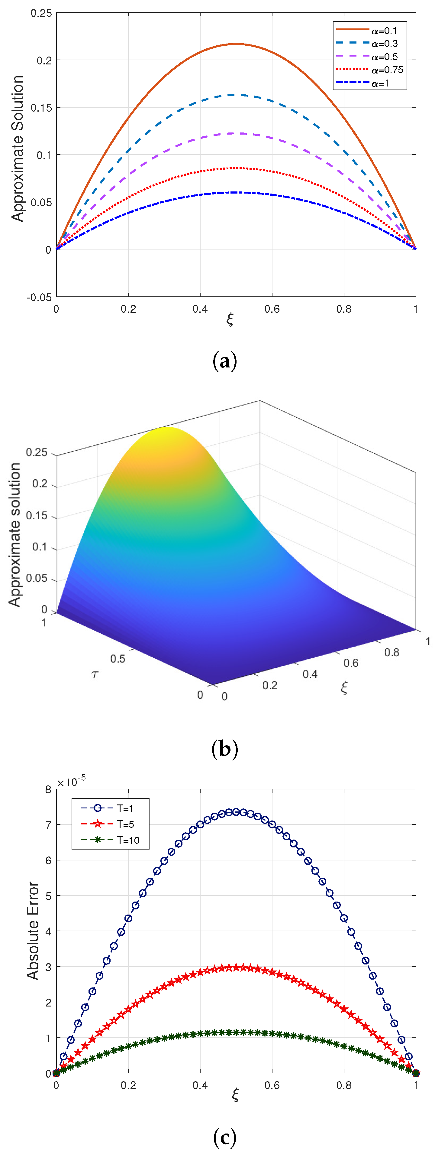
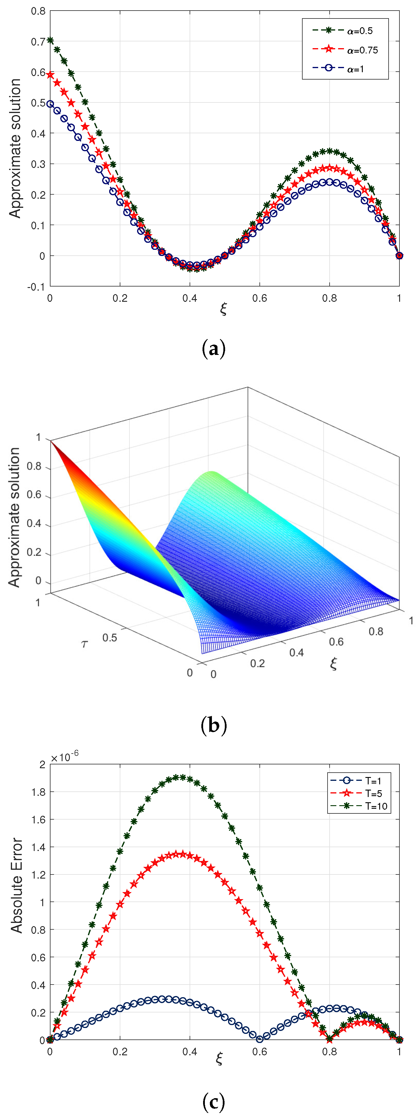
The initial and boundary conditions are extracted from the exact solution provided above. When $\alpha =0.5$,

Table 4. Comparison of error norms from Example 2 for different values of T when $0\le \xi \le 1$, $\alpha =0.5$, $M=100$, $\eta =0.5$, and $d\tau =0.0005$.

	M43BS		[24]		CPU Time (s)
T	${\mathit{L}}_{\mathbf{2}}$	${\mathit{L}}_{\infty }$	${\mathit{L}}_{\mathbf{2}}$	${\mathit{L}}_{\infty }$
1.0	2.311$\times {10}^{-7}$	3.172$\times {10}^{-7}$	$1.601\times {10}^{-7}$	$1.100\times {10}^{-6}$	2.38013
0.75	3.665$\times {10}^{-7}$	5.023$\times {10}^{-7}$	$5.603\times {10}^{-3}$	$2.460\times {10}^{-6}$	1.39935
0.5	6.824$\times {10}^{-7}$	9.348$\times {10}^{-7}$	$4.320\times {10}^{-8}$	$3.000\times {10}^{-7}$	0.76044
0.25	1.901$\times {10}^{-6}$	2.598$\times {10}^{-6}$	–	–	0.32101

displays the error norms comparison with the results reported in [24] at various time scales. The close agreement between the exact and numerical solutions can be observed from this table. By taking $\alpha =0.75$, $d\tau =0.01$,

Table 5. Error norms from Example 2 for different values of M when $0\le \xi \le 1$, $\alpha =0.75$, $\eta =0.5$, $d\tau =0.01$, and $T=0.5,1$.

	T = 0.5		T = 1
M	${\mathit{L}}_{\mathbf{2}}$	${\mathit{L}}_{\infty }$	${\mathit{L}}_{\mathbf{2}}$	${\mathit{L}}_{\infty }$
10	1.187$\times {10}^{-4}$	1.926$\times {10}^{-4}$	2.484$\times {10}^{-4}$	3.897$\times {10}^{-4}$
20	1.872$\times {10}^{-5}$	2.749$\times {10}^{-5}$	8.258$\times {10}^{-6}$	1.420$\times {10}^{-5}$
40	2.562$\times {10}^{-5}$	3.362$\times {10}^{-5}$	7.761$\times {10}^{-6}$	1.033$\times {10}^{-5}$
80	2.624$\times {10}^{-5}$	4.199$\times {10}^{-5}$	8.670$\times {10}^{-6}$	1.934$\times {10}^{-5}$
100	2.627$\times {10}^{-5}$	4.128$\times {10}^{-5}$	8.724$\times {10}^{-6}$	2.106$\times {10}^{-5}$

presents error norms for different numbers of divisions M across the spatial domain. The error norms go on decreasing with increases in the number of spatial partitions M.

Table 6. Error norms for Example 2 at $T=0.5$ for some values of $\alpha$ when $0\le \xi \le 1$, ${\left(d\tau \right)}_m={\displaystyle \frac{1}{2^{m+1}}}$, $\eta =0.5$, and $M=100$.

$\mathit{\alpha }$	m	$\mathit{d}\mathit{\tau }$	${\mathit{L}}_2$	${\mathit{L}}_{\mathit{\infty }}$
	1	0.25	1.815$\times {10}^{-2}$	2.377$\times {10}^{-2}$
	2	0.125	1.191$\times {10}^{-2}$	1.622$\times {10}^{-2}$
0.05	3	0.0625	5.714$\times {10}^{-3}$	8.684$\times {10}^{-3}$
	4	0.03125	2.909$\times {10}^{-3}$	5.421$\times {10}^{-3}$
	5	0.015625	1.794$\times {10}^{-3}$	3.724$\times {10}^{-3}$
	1	0.25	2.838$\times {10}^{-3}$	4.661$\times {10}^{-3}$
	2	0.125	1.133$\times {10}^{-3}$	2.227$\times {10}^{-3}$
0.95	3	0.0625	2.015$\times {10}^{-4}$	5.389$\times {10}^{-4}$
	4	0.03125	6.373$\times {10}^{-5}$	1.291$\times {10}^{-4}$
	5	0.015625	2.801$\times {10}^{-5}$	3.686$\times {10}^{-5}$

reports $L_2$ and $L_{\infty }$ error norms for various choices of $d\tau$, taking into account $M=100$ at time level $T=0.5$. It is evident from Table 6 that, with decreasing temporal step size, $L_2$ and $L_{\infty }$ error norms go on decreasing. For $M=40$, $d\tau =0.015$, and $\eta =0.5$, the 2-D surface behaviour of the suggested solution in the case of Example 2 at distinct values of fractional parameter $\alpha$ is shown in Figure 2a, and the three-dimensional representation of the proposed solution for $\alpha =0.5$ is depicted in Figure 2b. A 2-D plot for absolute error comparison at distinct temporal levels is displayed in Figure 2c for the parameters $\alpha =0.5$, $d\tau =0.0005$, and $M=50$. It is notable that the results obtained through present approach are in close agreement with the exact ones.

Example 3.

Examine the non-linear Equation (6) for $v_1=1$, ${\beta }_1=1$ and $p_1=1$ based on the initial condition

$$W(\xi ,0)=0,0\le \xi \le 1,$$

(48)

together with the end conditions

$$W(0,\tau )=0,W(1,\tau )=0,\tau \in [0,T].$$

(49)

The form of term $\mathtt{Z}(\xi ,\tau )$ is

$$\mathtt{Z}(\xi ,\tau )={\displaystyle \frac{2{\tau }^{2-\alpha }sin\left(2\pi \xi \right)}{\Gamma (3-\alpha )}}+2\pi {\tau }^{4}sin\left(2\pi \xi \right)cos\left(2\pi \xi \right)+4v_1{\pi }^2{\tau }^{2}sin\left(2\pi \xi \right).$$

(50)

The exact solution [41] of the problem is

$$W(\xi ,\tau )={\tau }^{2}sin\left(2\pi \xi \right).$$

(51)

Table 7. Comparison of error norms of Example 3 for different values of $v_1$ for $\alpha =0.5$, M = 120, $d\tau =0.0005$, and $T=0.1$.

		${\mathit{v}}_1=1$	${\mathit{v}}_1=0.5$	${\mathit{v}}_1=0.1$	${\mathit{v}}_1=0.01$	${\mathit{v}}_1=0.001$
M43BS	$L_2$	2.890$\times {10}^{-6}$	5.396$\times {10}^{-6}$	1.703$\times {10}^{-5}$	3.106$\times {10}^{-5}$	3.366$\times {10}^{-5}$
	$L_{\infty }$	4.088$\times {10}^{-6}$	7.631$\times {10}^{-6}$	2.408$\times {10}^{-5}$	4.392$\times {10}^{-5}$	4.759$\times {10}^{-5}$
CPU   Time (s)		0.15895	0.14446	0.14746	0.15882	0.14203
[42]	$L_2$	7.450$\times {10}^{-8}$	1.570$\times {10}^{-7}$	5.840$\times {10}^{-7}$	1.200$\times {10}^{-6}$	1.320$\times {10}^{-6}$
	$L_{\infty }$	1.100$\times {10}^{-7}$	2.300$\times {10}^{-7}$	8.580$\times {10}^{-7}$	1.800$\times {10}^{-6}$	2.010$\times {10}^{-6}$
[41]	$L_2$	2.910$\times {10}^{-5}$	2.660$\times {10}^{-5}$	1.500$\times {10}^{-5}$	1.040$\times {10}^{-6}$	-
	$L_{\infty }$	4.120$\times {10}^{-5}$	3.770$\times {10}^{-5}$	2.120$\times {10}^{-5}$	2.000$\times {10}^{-6}$	-

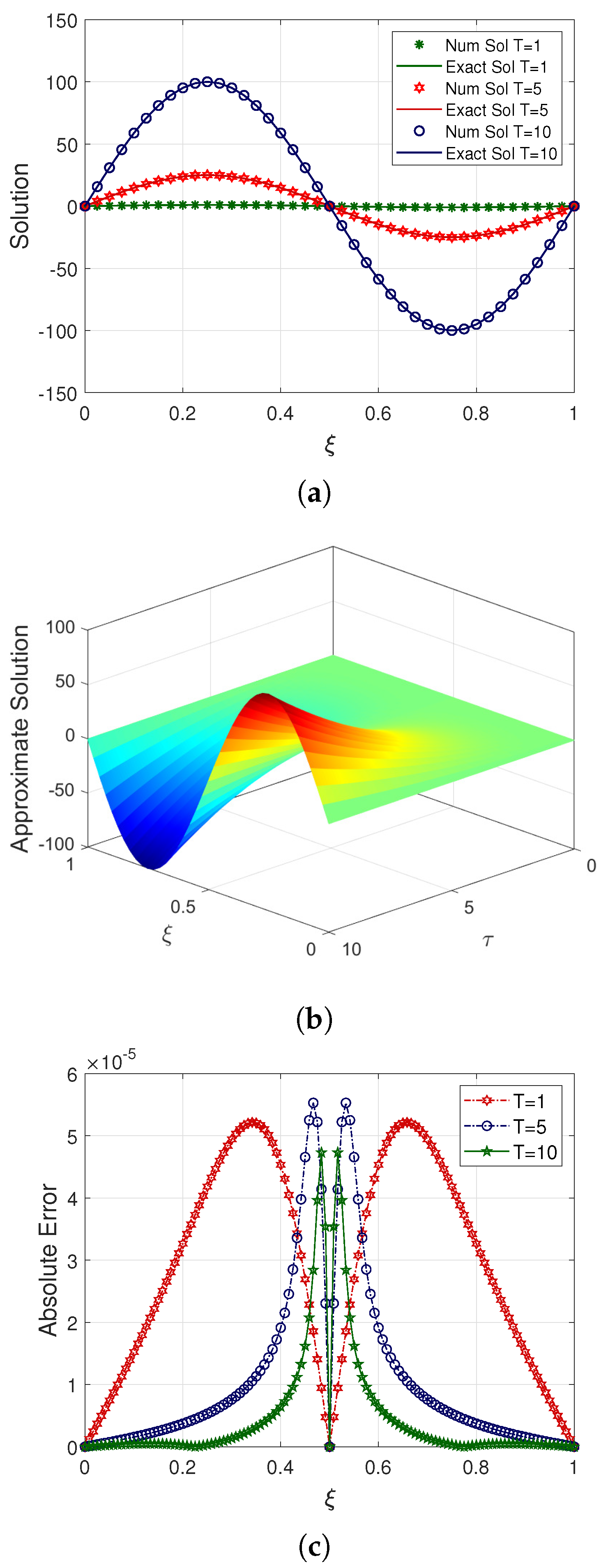
provides the comparison of error norms for some choices of viscosity parameter $v_1$ taking $\alpha =0.5$, $M=120$, and $d\tau =0.0005$ at time stage $T=0.1$, respectively. The order of convergence for spatial and temporal intervals is computed numerically in

Table 8. Order of convergence in the spatial domain at distinct temporal levels with d$\tau =0.001$ and $\alpha =0.85$.

M	T = 1		T = 2
ine	${\mathit{L}}_{\infty }$	Order	${\mathit{L}}_{\infty }$	Order
8	9.808$\times {10}^{-2}$	-	8.978$\times {10}^{-2}$	-
16	5.749$\times {10}^{-3}$	4.0923	7.717$\times {10}^{-3}$	3.5401
32	4.339$\times {10}^{-4}$	3.7279	3.880$\times {10}^{-4}$	4.3138
64	2.983$\times {10}^{-5}$	3.8624	2.336$\times {10}^{-5}$	4.0538
128	1.960$\times {10}^{-6}$	3.9277	1.240$\times {10}^{-6}$	4.2349

and

Table 9. Order of convergence in the temporal domain for different time levels with $M=100$ and $\alpha =0.75$.

$\mathit{d}\mathit{\tau }$	T = 1		T = 2		T = 5
ine	${\mathit{L}}_{\infty }$	Order	${\mathit{L}}_{\infty }$	Order	${\mathit{L}}_{\infty }$	Order
1	2.742$\times {10}^{-2}$	-	1.622$\times {10}^{-1}$	-	3.244$\times {10}^{-1}$	-
0.5	1.491$\times {10}^{-2}$	0.8785	4.124$\times {10}^{-2}$	1.9756	1.113$\times {10}^{-1}$	1.5426
0.25	5.498$\times {10}^{-3}$	1.4397	1.234$\times {10}^{-2}$	1.7398	4.455$\times {10}^{-2}$	1.3214
0.125	2.429$\times {10}^{-3}$	1.1784	4.354$\times {10}^{-3}$	1.5036	2.069$\times {10}^{-2}$	1.1063

, respectively, showing the agreement between numerical and theoretical results. The numerical and the exact results for $\alpha =0.1$, $M=40$, and $d\tau =0.01$ at different time levels are illustrated in Figure 3a. The 3-D surface plot of the physical behaviour for $\alpha =0.5$, $M=40$, and $d\tau =0.001$ is displayed in Figure 3b. For $\alpha =0.25$, Figure 3c depicts the absolute error at various time stages.

Example 4.

Assume the coefficients ${\beta }_1=0$, $v_1=1$, and ${\gamma }_1=1$ in Equation (8), and consider its resulting form depending upon the initial condition

$$W(\xi ,0)={\xi }^3,0\le \xi \le 1,$$

in addition to boundary conditions as

$$W(0,\tau )=0,W(1,\tau )=\tau +1,\tau \in [0,T].$$

The factor $\mathtt{Z}(\xi ,\tau )$ is written as follows:

$$\mathtt{Z}(\xi ,\tau )={\displaystyle \frac{{\xi }^3}{\Gamma (2-\alpha )}}{\tau }^{1-\alpha }-6\xi (\tau +1)-\left[(1-{\xi }^3(\tau +1))({\xi }^3(\tau +1)-\eta )\right]{\xi }^3(\tau +1).$$

The exact solution [43] of the example is as follows:

$$W(\xi ,\tau )={\xi }^3(\tau +1).$$

Table 10. Error norms of Example 4 for different values of T by choosing $M=100$, $d\tau =0.01$, and $\alpha =0.5,0.75$.

	$\mathit{\alpha }=0.5$		$\mathit{\alpha }=0.75$
T	${\mathit{L}}_{\mathbf{2}}$	${\mathit{L}}_{\infty }$	${\mathit{L}}_{\mathbf{2}}$	${\mathit{L}}_{\infty }$
0.08	1.834$\times {10}^{-5}$	2.706$\times {10}^{-4}$	2.133$\times {10}^{-4}$	3.044$\times {10}^{-4}$
0.10	1.645$\times {10}^{-4}$	2.413$\times {10}^{-4}$	1.839$\times {10}^{-4}$	2.617$\times {10}^{-4}$
0.50	7.393$\times {10}^{-5}$	1.063$\times {10}^{-4}$	4.943$\times {10}^{-5}$	7.048$\times {10}^{-5}$
0.80	5.774$\times {10}^{-5}$	8.307$\times {10}^{-5}$	3.286$\times {10}^{-5}$	4.696$\times {10}^{-5}$
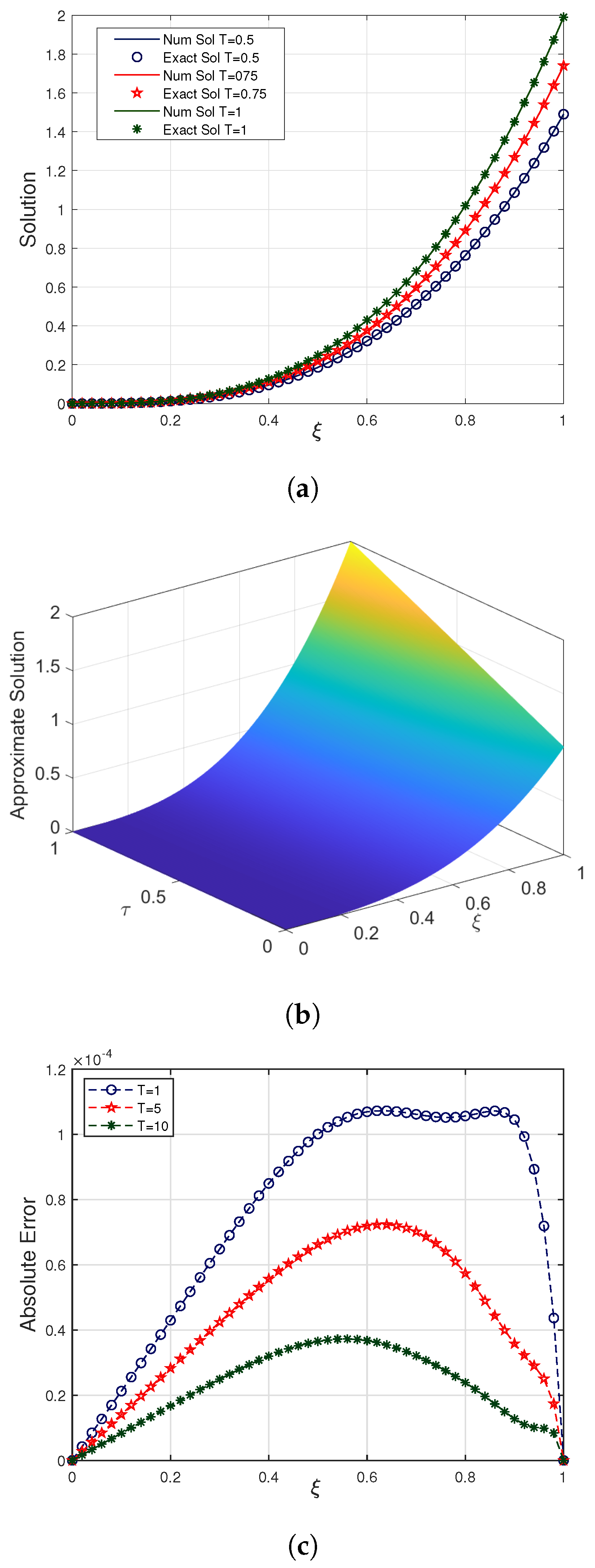
1.00	5.106$\times {10}^{-5}$	7.343$\times {10}^{-5}$	2.695$\times {10}^{-5}$	3.854$\times {10}^{-5}$

reports Euclidean error norm $L_2$ and maximum error norm $L_{\infty }$ for Example 4 at distinct temporal levels by choosing $\eta =0.5$, $h=0.01$, and d$\tau =0.01$, respectively. For few choices of spatial divisions M,

Table 11. Error norms for Example 4 at $T=1$ for some values of $\alpha$ when $0\le \xi \le 1$, ${\left(h\right)}_m={\displaystyle \frac{1}{2^{m+1}}}$, and $d\tau =0.01$.

$\mathit{\alpha }$	m	h	${\mathit{L}}_2$	${\mathit{L}}_{\mathit{\infty }}$
	1	0.25	8.059$\times {10}^{-5}$	1.108$\times {10}^{-5}$
	2	0.125	8.073$\times {10}^{-5}$	1.243$\times {10}^{-5}$
0.05	3	0.0625	8.085$\times {10}^{-5}$	1.281$\times {10}^{-4}$
	4	0.03125	8.087$\times {10}^{-5}$	1.281$\times {10}^{-4}$
	5	0.015625	8.087$\times {10}^{-5}$	1.281$\times {10}^{-4}$
	1	0.25	6.957$\times {10}^{-5}$	9.779$\times {10}^{-5}$
	2	0.125	6.969$\times {10}^{-5}$	9.907$\times {10}^{-5}$
0.25	3	0.0625	6.971$\times {10}^{-5}$	1.005$\times {10}^{-4}$
	4	0.03125	6.971$\times {10}^{-5}$	1.005$\times {10}^{-4}$
	5	0.015625	6.971$\times {10}^{-5}$	1.006$\times {10}^{-4}$

provides the error norms for Example 4, taking into account $\eta =0.5$, $d\tau =0.01$ at temporal scale $T=1$, respectively. According to Table analysis, the decrease in $L_2$ and $L_{\infty }$ error norms is the result of an increase in the number of spatial divisions M. Numerical comparison through absolute error across various knot points is shown in

Table 12. Comparison of the absolute error of Example 4 at different values of $\alpha$ when $0\le \xi \le 1$, $N=40$, $M=40$, $\eta =0.5$, and $T=0.1,0.01$.

T	$\mathit{\xi }$	$\mathit{\alpha }=0.6$	$\mathit{\alpha }=0.8$	$\mathit{\alpha }=1$
0.1	0.1	1.116$\times {10}^{-5}$	1.214$\times {10}^{-5}$	1.294$\times {10}^{-6}$
	0.3	3.347$\times {10}^{-5}$	3.571$\times {10}^{-5}$	3.476$\times {10}^{-6}$
	0.5	5.330$\times {10}^{-5}$	5.487$\times {10}^{-5}$	4.477$\times {10}^{-6}$
	0.7	6.091$\times {10}^{-5}$	5.972$\times {10}^{-5}$	3.767$\times {10}^{-6}$
	0.9	3.532$\times {10}^{-4}$	3.264$\times {10}^{-5}$	1.460$\times {10}^{-6}$
0.01	0.1	2.177$\times {10}^{-6}$	9.908$\times {10}^{-7}$	1.858$\times {10}^{-8}$
	0.3	7.260$\times {10}^{-6}$	4.448$\times {10}^{-6}$	5.571$\times {10}^{-8}$
	0.5	1.347$\times {10}^{-5}$	1.142$\times {10}^{-5}$	9.352$\times {10}^{-8}$
	0.7	1.783$\times {10}^{-5}$	1.932$\times {10}^{-5}$	1.267$\times {10}^{-7}$
	0.9	1.163$\times {10}^{-5}$	1.437$\times {10}^{-5}$	8.047$\times {10}^{-7}$

for different values of fractional order $\alpha$, considering $\eta =0.5$, $N=40$, and $M=40$. Table 12 reveals that increasing values of fractional order $\alpha$ contribute to a convergent solution. The result of utilizing various choices of time stages T, overlapping of the exact solution with numerical values in case of Example 4, and considering $d\tau =0.01$ and $h=0.025$ is illustrated in Figure 4a. A 3-D graphical representation of the numerical solution for $\alpha =0.75$, $d\tau =0.01$, $M=100$, and $\tau \in [0,1]$ is shown in Figure 4b. Furthermore, the absolute error profile resulting from taking $\alpha =0.05$, $M=50$, and $d\tau =0.01$ is depicted in Figure 4c. It is important to mention that the results achieved through the proposed methodology adequately capture the exact profile over the specified domain.

Example 5.

Consider the generalized form of the fractional Burgers’ Equation (6) by assuming parameters $p_1=3$, $v_1=1$, and ${\beta }_1=1$ subject to the initial condition

$$W(\xi ,0)=0,0\le \xi \le 1,$$

(52)

and the boundary conditions as

$$W(0,\tau )=0,W(1,\tau )=0,\tau \ge 0.$$

(53)

The form of term $\mathtt{Z}(\xi ,\tau )$ is

$$\begin{array}{cc}\hfill \mathtt{Z}(\xi ,\tau )=& {\displaystyle \frac{2\xi (\xi -1){\tau }^{2-\alpha }}{\Gamma (3-\alpha )}}-2v_1{\tau }^2+(2\xi -1){\tau }^2{\left(({\xi }^2-\xi ){\tau }^2\right)}^3.\hfill \end{array}$$

The exact solution of the considered problem is given by [44]:

$$W(\xi ,\tau )=\xi (\xi -1){\tau }^2.$$

(54)

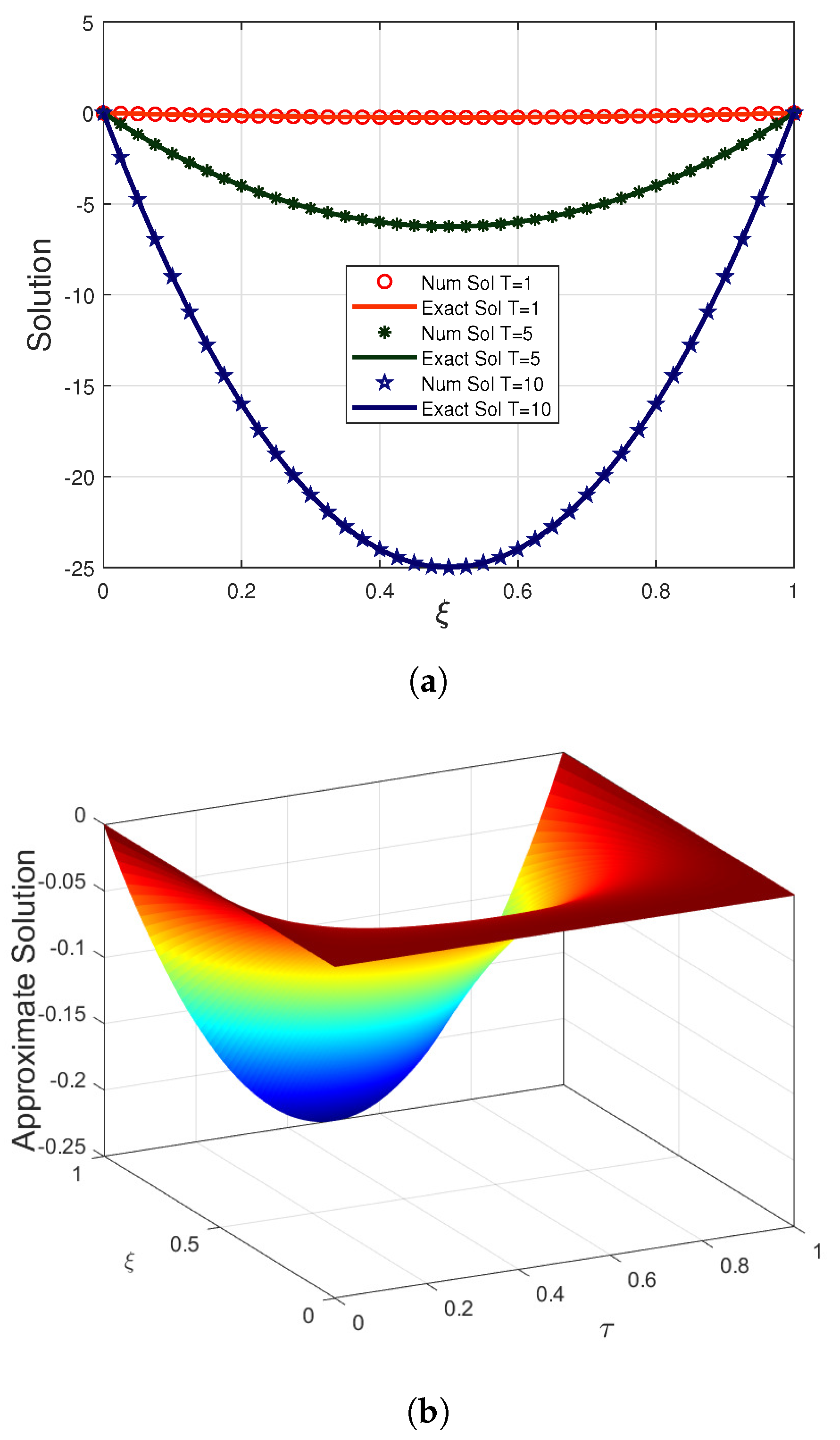
The computation of $L_2$ as well as $L_{\infty }$ norms for $\alpha =0.25,0.75$ is reported in

Table 13. Error norms for distinct temporal scales with $d\tau =0.001$ and $h=0.01$.

T	$\mathit{\alpha }=0.25$		$\mathit{\alpha }=0.75$
ine	${\mathit{L}}_{\infty }$	${\mathit{L}}_{\mathbf{2}}$	${\mathit{L}}_{\infty }$	${\mathit{L}}_{\mathbf{2}}$
0.25	8.529$\times {10}^{-5}$	6.055$\times {10}^{-5}$	1.192$\times {10}^{-4}$	8.473$\times {10}^{-5}$
0.5	1.477$\times {10}^{-4}$	1.049$\times {10}^{-4}$	1.646$\times {10}^{-4}$	1.168$\times {10}^{-4}$
0.75	2.030$\times {10}^{-4}$	1.442$\times {10}^{-4}$	1.936$\times {10}^{-4}$	1.375$\times {10}^{-4}$
1	2.542$\times {10}^{-4}$	1.805$\times {10}^{-4}$	2.155$\times {10}^{-4}$	1.530$\times {10}^{-4}$

, taking into account $h=0.01$, $M=100$, and $d\tau =0.01$. From this table, it can be clearly observed that as the value of $\alpha$ approaches 1, the estimated solution tends to exactly one. The close similarity between the exact solution and estimated outcomes obtained by the proposed approach at distinct temporal scales is provided in Figure 5a, taking $\alpha =0.5$, $M=40$, and $d\tau =0.01$. The graphical illustration of the proposed solution in three dimensions at $\alpha =0.25$, $M=100$, and $d\tau =0.01$ is shown in Figure 5b. Further, it is concluded that the exact findings and numerical outcomes of the proposed approach are compatible with each other.

7. Conclusions

In this work, the modified cubic splines approximation is successfully applied to solve a Burgers’-Huxley model of fractional order. The finite difference technique is applied to approximate the fractional-order operator in the temporal direction, and a cubic B-spline basis is employed to interpolate the spatial domain. To demonstrate the capability of present technique, five different test examples are successfully solved. The von Neumann stability analysis is utilized to establish the unconditional stability. The effectiveness of approach is validated using $L_2$ and $L_{\infty }$ error norms in addition to graphical as well as tabular representation of numerical outcomes. The solution profiles clearly show the matching of numerical and exact results for several selections of fractional parameter $\alpha$. Based on the results, it can be inferred that the $M43BS$ technique is easy to implement and elegant for solving higher-order partial differential equations having fractional derivatives in spatial and temporal directions. Future research will focus on extending the proposed approach to multi-dimensional and coupled fractional PDEs to investigate their impact on mathematical modeling and numerical behaviour, particularly for problems with non-standard boundary conditions and variable coefficients. Additionally, the method will be applied to real-world physical, biological, and engineering systems governed by nonlinear PDEs to demonstrate its robustness, efficiency, and versatility.

References

1. Javaid, M.; Tahir, M.; Imran, M.; Baleanu, D.; Akgul, A.; Imran, M.A. Unsteady flow of fractional Burgers’ fluid in a rotating annulus region with power law kernel. Alexandria Eng. J. 2022, 6, 17–27. [Google Scholar] [CrossRef]
2. He, J.H. Approximate analytical solution for seepage flow with fractional derivatives in porous media. Comput. Methods Appl. Mech. Eng. 1998, 167, 57–68. [Google Scholar] [CrossRef]
3. Sahraoui, S.; Zekri, N. On fractional modeling of viscoelastic foams. Mech. Res. Commun. 2019, 96, 62–66. [Google Scholar] [CrossRef]
4. Tarasov, V.E. On history of mathematical economics: Application of fractional calculus. Mathematics 2019, 7, 509. [Google Scholar] [CrossRef]
5. Wang, X.Y.; Zhu, Z.S.; Lu, Y.K. Solitary wave solutions of the generalised Burgers—Huxley equation. J. Phys. A. Math. Gen. 1990, 23, 271–274. [Google Scholar] [CrossRef]
6. Bateman, H. Some recent researches on the motion of fluids. Mon. Weather Rev. 1915, 43, 163–170. [Google Scholar] [CrossRef]
7. Burgers, J.M. A mathematical model illustrating the theory of turbulence. Adv. Appl. Mech. 1948, 1, 171–199. [Google Scholar]
8. Freihet, A.A.; Zuriqat, M. Analytical solution of fractional Burgers—Huxley equations via residual power series method. Lobachevskii J. Math. 2019, 40, 174–182. [Google Scholar] [CrossRef]
9. Taniuti, T. Reductive perturbation method and far fields of wave equations. Prog. Theor. Phys. Suppl. 1974, 55, 1–35. [Google Scholar] [CrossRef]
10. Wang, X.Y. Nerve propagation and wall in liquid crystals. Phys. Lett. A 1985, 112, 402–406. [Google Scholar] [CrossRef]
11. Herrmann, R. Fractional Calculus: An Introduction for Physicists, 2nd ed.; World Scientific: Singapore, 2014. [Google Scholar]
12. Podlubny, I. Fractional Differential Equations; Academic Press: San Diego, CA, USA, 1999. [Google Scholar]
13. Caputo, M. Linear models of dissipation whose Q is almost frequency independent-II. Geophys. J. Roy Astr. Soc. 1967, 13, 529–539. [Google Scholar] [CrossRef]
14. Hilfer, R. Applications of Fractional Calculus in Physics; World Scientific: Singapore, 2000. [Google Scholar]
15. Caputo, M.; Fabrizio, M. A new definition of fractional derivative without singular kernel. Progr. Fract. Differ. Appli. 2015, 1, 73–85. [Google Scholar]
16. Atangana, A. Derivative with a New Parameter: Theory, Methods and Applications; Academic Press: San Diego, CA, USA, 2016. [Google Scholar]
17. Mohanty, R.K.; Dai, W.; Liu, D. Operator compact method of accuracy two in time and four in space for the solution of time dependent Burgers’-Huxley equation. Numer. Algorithms 2015, 70, 591–605. [Google Scholar] [CrossRef]
18. Inc, M.; Yusuf, A.; Aliyu, A.I.; Baleanu, D. Lie symmetry analysis and explicit solutions for the time fractional generalized Burgers’-Huxley equation. Opt. Quantum Electron 2018, 50, 1–16. [Google Scholar] [CrossRef]
19. Inc, M.; Partohaghighi, M.; Akinlar, M.A.; Agarwal, P.; Chu, Y. New solutions of fractional-order Burgers’-Huxley equation. Results Phys. 2020, 18, 1–5. [Google Scholar] [CrossRef]
20. Kumar, S.; Pandey, P. A Legendre spectral finite difference method for the solution of non-linear space-time fractional Burgers’-Huxley and reaction-diffusion equation with Atangana–Baleanu derivative. Chaos Solitons Fractals 2020, 130, 1–7. [Google Scholar]
21. Alquran, M.; Khaled, K.; Sivasundaram, S.; Jaradat, H.M. Mathematical and numerical study of existence of bifurcations of the generalized fractional Burgers’-Huxley equation. J. Nonlinear Stud. 2017, 24, 235–244. [Google Scholar]
22. Tripathi, N.K. Analytical solution of two dimensional nonlinear space–time fractional Burgers’-Huxley equation using fractional sub-equation method. Natl. Acad. Sci. Lett. 2018, 41, 295–299. [Google Scholar] [CrossRef]
23. Heydari, M.H.; Avazzadeh, Z. Fibonacci polynomials for the numerical solution of variable-order space-time fractional Burgers-Huxley equation. Math. Meth. Appl. Sci. 2021, 44, 6774–6786. [Google Scholar] [CrossRef]
24. Majeed, A.; Kamran, M.; Asghar, N.; Baleanu, D. Numerical approximation of inhomogeneous time fractional Burgers’-Huxley equation with B-spline functions and Caputo derivative. J. Eng. Comput. 2022, 38, 885–900. [Google Scholar] [CrossRef]
25. Kanth, V.R.; Aruna, K.; Raghavendar, K. Natural transform decomposition method for the numerical treatment of the time fractional Burgers–Huxley equation. Numer. Meth. Partial Diff. Equ. 2022, 39, 2690–2718. [Google Scholar] [CrossRef]
26. Yang, X.; Liu, X. Numerical analysis of fourth-order compact difference scheme for inhomogeneous time-fractional Burgers-Huxley equation. Comp. Math. Appl. 2022, 125, 1–12. [Google Scholar] [CrossRef]
27. Akram, T.; Iqbal, A.; Kumam, P.; Sutthibutpong, T. A newly constructed numerical approximation and analysis of Generalized fractional Burger-Huxley equation using higher order method. Results Phys. 2023, 54, 107119. [Google Scholar] [CrossRef]
28. Habiba, U.; Salam, M.A.; Khan, K. Stability, Bifurcation, and Traveling Wave Solutions to the Generalized Time-Fractional Burgers-Huxley Equation. Int. J. Appl. Comput. Math. 2024, 10, 62. [Google Scholar] [CrossRef]
29. Arifeen, S.U.; Haq, S.; Ali, I. Galerkin approximation of Burgers-Huxley equation with fractional order arising in reaction mechanism and diffusion transport. Phys. Scr. 2024, 99, 125215. [Google Scholar] [CrossRef]
30. Huang, Z.; Huang, Y. Dynamics of fractional stochastic Burgers–Huxley equation with Lévy noise. Results Phys. 2025, 73, 108235. [Google Scholar] [CrossRef]
31. Abali, S.; Konuralp, A. Solutions of Volterra-Fredholm type fractional integro-differential equations in terms of shifted Gegenbauer wavelets compared with the solutions by Genocchi polynomial method. J. Comput. Appl. Math. 2025, 476, 117056. [Google Scholar] [CrossRef]
32. Gurbuz, B.; Sezer, M. Modified operational matrix method for second-order nonlinear ordinary differential equations with quadratic and cubic terms. Int. J. Opt. Control Theor. Appl. 2020, 10, 218–225. [Google Scholar]
33. Khan, M.N.; Ahmad, M.; Jan, R.; Ahmad, I.; Mousa, M. Solving parabolic differential equations via Haar wavelets: A focus on integral boundary conditions. Int. J. Opt. Control Theor. Appl. 2025, 15, 594–609. [Google Scholar] [CrossRef]
34. Prenter, P.M. Splines and Variational Methods; Wiley-Interscience Publication: New York, NY, USA, 1975. [Google Scholar]
35. Daniel, J.W.; Swartz, B.K. Extrapolated collocation for two-point boundary-value problems using cubic splines. IMA J. Appl. Math. 1975, 16, 161–174. [Google Scholar] [CrossRef]
36. Lucas, T.R. Error bounds for interpolating cubic splines under various end conditions. SIAM J. Numer. Anal. 1974, 11, 569–584. [Google Scholar] [CrossRef]
37. Liu, F.; Zhuang, P.; Anh, V.; Turner, I.; Burrage, K. Stability and convergence of the difference methods for the space time fractional advection-diffusion equation. Appl. Math. Comput. 2007, 191, 12–20. [Google Scholar] [CrossRef]
38. Lin, Y.; Xu, C. Finite difference/spectral approximations for the time fractional diffusion equation. J. Comput. Phys. 2007, 225, 1533–1552. [Google Scholar] [CrossRef]
39. Bellman, R.E.; Kalaba, R.E. Quasilinearization and Nonlinear Boundary Value Problems; Elsevier: New York, NY, USA, 1965. [Google Scholar]
40. Lopez-Marcos, J.C. A difference scheme for a nonlinear partial integro differential equation. SIAM J. Numer. Anal. 1990, 27, 20–31. [Google Scholar] [CrossRef]
41. Esen, A.; Tasbozan, O. Numerical solution of time fractional Burgers equation. Acta Univ. Sapientiae Math. 2015, 7, 167–185. [Google Scholar] [CrossRef]
42. Singh, B.K.; Gupta, M. Trigonometric tension B-spline collocation approximations for time fractional Burgers’ equation. J. Ocean Eng. Sci. 2022, 9, 508–516. [Google Scholar] [CrossRef]
43. Hadhoud, A.R.; Abd Alaal, F.E.; Abdelaziz, A.A.; Radwan, T. Numerical treatment of the generalized time-fractional Huxley-Burgers’ equation and its stability examination. Demonstr. Math. 2021, 54, 436–451. [Google Scholar] [CrossRef]
44. Majeed, A.; Kamran, M.; Rafique, M. An approximation to the solution of time fractional modified Burgers’ equation using extended cubic B-spline method. Comput. Appl. Math. 2020, 39, 257. [Google Scholar] [CrossRef]
Figure 1. (a) Solution profile at temporal stage T = 0.5 for different choices of α ; (b) 3-D surface behaviour for α = 0.5 and τ [ 0 , 1 ] ; (c) absolute error plot at α = 0.5 for various time levels.
Fractalfract 09 00780 g001
Figure 2. (a) Solution behaviour at time level T = 0.5 for particular values of α ; (b) 3-D graphical preview of the solution for α = 0.5 , M = 100 , d τ = 0.0005 , and τ ∈[0, 1]; (c) 2 − D error plot for α = 0.5 at different time levels.
Fractalfract 09 00780 g002
Figure 3. (a) Solution profile for α = 0.1 at different time levels; (b) 3-D surface behaviour for α = 0.5 ; (c) absolute error plot at α = 0.25 for various time levels.
Fractalfract 09 00780 g003
Figure 4. (a) Solution profile at α = 0.5 for various values of T; (b) 3-D representation of physical behaviour of the solution for α = 0.75 , and T 1 ; (c) absolute error plot for α = 0.05 at different time levels.
Fractalfract 09 00780 g004
Figure 5. (a) Solution behaviour at α = 0.5 for distinct values of T; (b) 3-D plot of the numerical solution at α = 0.25 and T 1 .
Fractalfract 09 00780 g005