Solving Helmholtz Equation with Local Fractional Derivative Operators


1
Department of Mathematics, Çankaya University, 06530 Ankara, Turkey
2
Institute of Space Sciences, Magurele, 077125 Bucharest, Romania
3
Department of Mathematics and Statistics, Faculty of Science, Tshwane University of Technology, Private Bag X680, Pretoria 0001, South Africa
4
Department of Mathematics, Faculty of Education for Pure Sciences University of Thi-Qar, Nasiriyah 64001, Iraq
5
Department of Mathematics, College of Science, King Saud University, P. O. BOX 2454, Ryad 11451, Saudia Arabia
*
Author to whom correspondence should be addressed.
Fractal Fract. 2019, 3(3), 43; https://doi.org/10.3390/fractalfract3030043
Submission received: 3 July 2019
/
Revised: 20 July 2019
/
Accepted: 23 July 2019
/
Published: 1 August 2019
Abstract
:The paper presents a new analytical method called the local fractional Laplace variational iteration method (LFLVIM), which is a combination of the local fractional Laplace transform (LFLT) and the local fractional variational iteration method (LFVIM), for solving the two-dimensional Helmholtz and coupled Helmholtz equations with local fractional derivative operators (LFDOs). The operators are taken in the local fractional sense. Two test problems are presented to demonstrate the efficiency and the accuracy of the proposed method. The approximate solutions obtained are compared with the results obtained by the local fractional Laplace decomposition method (LFLDM). The results reveal that the LFLVIM is very effective and convenient to solve linear and nonlinear PDEs.
1. Introduction
The Helmholtz equation often arises in the study of physical problems involving partial differential equation (PDEs) in both space and time. The Helmholtz equation with local fractional derivative operators in two-dimensional case was suggested in [1,2] as follows:
with the initial value conditions as follows:
where is the unknown function and is a source term. While coupled Helmholtz equations with local fractional derivative operators in two-dimensional case was introduced in [2] as follows:
subject to the initial conditions:
where and are unknown functions and and are source terms.
In recent years, many of the approximate and analytical methods have been utilized to solve the PDEs with LFDOs such as the Adomian decomposition method [3,4,5], variational iteration method [6,7,8,9,10,11], differential transform method [12,13], series expansion method [14,15,16], Sumudu transform method [17], Fourier transform method [18], function decomposition method [19,20], Laplace transform method [21,22], reduce differential transform method [23,24], homotopy perturbation Sumudu transform [25], and the existence and uniqueness of solutions for local fractional differential equations [26,27].
The main aim of this work is to propose the local fractional Laplace variational iteration method to solve Helmholtz and coupled Helmholtz equations with LFDOs. It is important to note that the new modification reduces the size of calculations compared to the LFVIM. This paper is organized as follows: In Section 2, the basic mathematical tools of local fractional calculus are introduced. The analysis of the proposed method is given in Section 3. Then in Section 4, the proposed method is implemented to solve some examples. Finally, concluding remarks are presented in Section 5.
2. Basic Definitions of Local Fractional Calculus
In this section, we introduce the basic definitions and properties of the local fractional calculus used to describe the proposed schemes.
Definition 2.
If the functions are local fractional continuous then the local fractional derivatives and integrals exist.
Definition 3.
Theorem 1.
Suppose thatandthen we have the following formulas:
Proof of Theorem 1:
see [29].
Theorem 2.
Letand, then
3. Analysis of the Method
In this section, we illustrate the basic idea of the Laplace variational iteration method for the local fractional partial differential equation.
Let us consider the following local fractional partial differential equations:
where is the linear LFDO, is a linear LFDO of order less than , represents the general nonlinear LFDO, and is the source term.
According to the rule of LFVIM, the correction local fractional functional for Equation (16) is constructed as [6,7,8,9,10,30,31]:
where is a fractal Lagrange multiplier.
For initial value problems of Equation (16), we can start with:
We now take the Yang-Laplace transform of Equation (17), namely:
or
Taking the local fractional variation of Equation (20), which is given by:
By using the computation of Equation (21), we get:
Hence, from Equation (22) we get:
where:
Therefore, we get:
Therefore, we have the following iteration algorithm:
where the initial value reads as:
Thus, the local fractional series solution of Equation (16) is:
4. Illustrated Examples
In order to illustrate the above results in Section 3, we give the following several examples.
Example 1.
Let us consider the following Helmholtz equation involving the local fractional operator:
with the initial value conditions as follows:
Using relation Equation (26), we structure the iterative relation as:
In view of Equation (27), the initial value reads:
Making use of Equations (31) and (32), the successive approximate solutions are shown as follows:
The result is the same as the one that is obtained by the LFLDM [2].
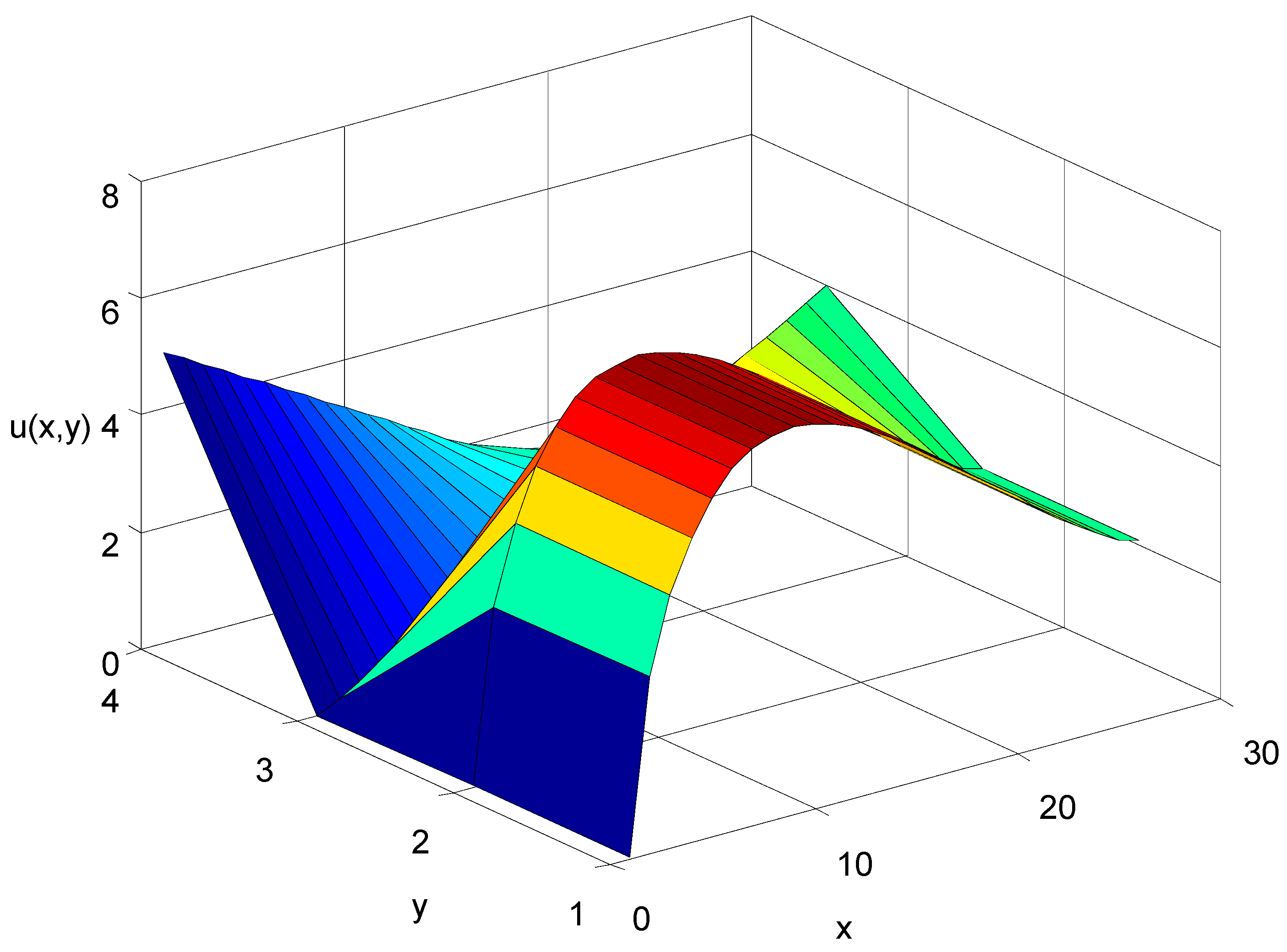
In Figure 1, Figure 2 and Figure 3, the three-dimensional plots of the approximate solutions of Equation (29) with initial condition Equation (30) are shown for different values of , respectively.
Example 2.
Consider the coupled Helmholtz equations with the local fractional derivative operators:
subject to the initial conditions:
In view of Equations (26) and (34), the local fractional iteration algorithm can be written as follows:
which leads to:
where the initial value reads:
Making use of Equations (37) and (38), the successive approximate solutions are shown as follows:
Consequently, the local fractional series solution is:
5. Conclusions
In this work we utilized the coupling method of the local fractional variational iteration method and Laplace transform to solve Helmholtz and coupled Helmholtz equations and their approximate solutions were obtained. The local fractional Laplace variational iteration method was proved to be an effective approach for solving partial differential equations with local fractional derivative operators due to the excellent agreement between the obtained approximate solution and the exact solution. A comparison was made to show that the method has a small size of computation in comparison with the computational size required in other numerical methods, and its rapid convergence shows that the method is reliable and introduces a significant improvement in solving linear and nonlinear partial differential equations with local fractional derivative operators.
Author Contributions
H.K.J. wrote some sections of the manuscript; D.B. and M.A. prepared some other sections of the paper and performed analyses. All authors have read and approved the final manuscript.
Funding
This research received no external funding.
Acknowledgments
The authors are very grateful to the referees for useful comments and suggestions towards the improvement of this paper.
Conflicts of Interest
The authors declare no conflict of interest.
References
- Hao, Y.; Srivastava, H.M.; Jafari, H.; Yang, X.J. Helmholtz and diffusion equations associated with local fractional derivative operators involving the Cantorian and Cantor-type cylindrical coordinates. Adv. Math. Phys. 2013, 2013, 754248. [Google Scholar] [CrossRef]
- Jassim, H.K. The approximate solutions of helmholtz and coupled helmholtz equations on cantor sets within local fractional operator. J. Zankoy Sulaimani Part A 2015, 17, 19–25. [Google Scholar] [CrossRef]
- Baleanu, D.; Jassim, H.K.; Qurashi, M.A. Approximate analytical solutions of goursat problem within local fractional operators. J. Nonlinear Sci. Appl. 2016, 9, 4829–4837. [Google Scholar] [CrossRef]
- Fan, Z.P.; Jassim, H.K.; Raina, R.K.; Yang, X.-J. Adomian decomposition method for three-dimensional diffusion model in fractal heat transfer involving local fractional derivatives. Therm. Sci. 2015, 19, S137–S141. [Google Scholar] [CrossRef]
- Jafari, H.; Jassim, H.K. Local fractional adomian decomposition method for solving two dimensional heat conduction equations within local fractional operators. J. Adv. Math. 2014, 9, 2574–2582. [Google Scholar]
- Baleanu, D.; Jassim, H.K.; Khan, H. A modification fractional variational iteration method for solving nonlinear gas dynamic and coupled KdV equations involving local fractional operators. Therm. Sci. 2018, 19, S165–S175. [Google Scholar] [CrossRef]
- Baleanu, D.; Jassim, H.K. Approximate solutions of the damped wave equation and dissipative wave equation in fractal strings. Fractal Fract. 2019, 3, 26. [Google Scholar] [CrossRef]
- Jafari, H.; Jassim, H.K. Local fractional variational iteration method for nonlinear partial differential equations within local fractional operators. Appl. Appl. Math. 2015, 10, 1055–1065. [Google Scholar]
- Xu, S.; Ling, X.; Zhao, Y.; Jassim, H.K. A novel schedule for solving the two-dimensional diffusion in fractal heat transfer. Therm. Sci. 2015, 19, S99–S103. [Google Scholar] [CrossRef]
- Jafari, H.; Jassim, H.K.; Vahidi, J. Reduced differential transform and variational iteration methods for 3D diffusion model in fractal heat transfer within local fractional operators. Therm. Sci. 2018, 22, S301–S307. [Google Scholar] [CrossRef]
- Jassim, H.K.; Shahab, W.A. Fractional variational iteration method to solve one dimensional second order hyperbolic telegraph equations. J. Phys. Conf. Ser. 2018, 1032, 1–9. [Google Scholar] [CrossRef]
- Yang, X.J.; Machad, J.A.; Srivastava, H.M. A new numerical technique for solving the local fractional diffusion equation: Two-dimensional extended differential transform approach. Appl. Math. Comput. 2016, 274, 143–151. [Google Scholar] [CrossRef]
- Jafari, H.; Jassim, H.K.; Tchier, F.; Baleanu, D. On the approximate solutions of local fractional differential equations with local fractional operator. Entropy 2016, 18, 150. [Google Scholar] [CrossRef]
- Baleanu, D.; Jassim, H.K. A novel approach for Korteweg-de Vries equation of fractional order. J. Appl. Comput. Mech. 2019, 5, 192–198. [Google Scholar]
- Yang, A.-M.; Yang, X.-J.; Li, Z.-B. Local fractional series expansion method for solving wave and diffusion equations Cantor sets. Abstr. Appl. Anal. 2013, 2013, 351057. [Google Scholar] [CrossRef]
- Jassim, H.K. On approximate methods for fractal vehicular traffic flow. TWMS J. Appl. Eng. Math. 2017, 7, 58–65. [Google Scholar]
- Srivastava, H.M.; Golmankhaneh, A.K.; Baleanu, D. Local fractional sumudu transform with application to IVPs on Cantor Set. Abstr. Appl. Anal. 2014, 2014, 620529. [Google Scholar] [CrossRef]
- Hu, M.-S.; Agarwal, R.P.; Yang, X.-J. Local fractional fourier series with application to wave equation in fractal vibrating. Abstr. Appl. Anal. 2012, 2012, 567401. [Google Scholar] [CrossRef]
- Wang, S.Q.; Yang, Y.J.; Jassim, H.K. Local fractional function decomposition method for solving inhomogeneous wave equations with local fractional derivative. Abstr. Appl. Anal. 2014, 2014, 176395. [Google Scholar] [CrossRef]
- Yan, S.P.; Jafari, H.; Jassim, H.K. Local fractional adomian decomposition and function decomposition methods for solving laplace equation within local fractional operators. Adv. Math. Phys. 2014, 2014, 161580. [Google Scholar] [CrossRef]
- Jassim, H.K. The analytical solutions for volterra integro-differential equations involving local fractional operators by yang-laplace transform. Sahand Commun. Math. Anal. 2017, 6, 69–76. [Google Scholar]
- Zhao, C.G.; Yang, A.-M.; Jafari, H.; Haghbin, A. The Yang-Laplace transform for solving the IVPs with local fractional derivative. Abstr. Appl. Anal. 2014, 2014, 386459. [Google Scholar] [CrossRef]
- Jafari, H.; Jassim, H.K.; Moshokoa, S.P.; Ariyan, V.M.; Tchier, F. Reduced differential transform method for partial differential equations within local fractional derivative operators. Adv. Mech. Eng. 2016, 8, 1–6. [Google Scholar] [CrossRef]
- Jassim, H.K. An efficient technique for solving linear and nonlinear wave equation within local fractional operators. J. Hyperstruct. 2017, 6, 136–146. [Google Scholar]
- Ait, T.; Hammouch, Z.; Mekkaoui, T.; Belgacem, F.B.M. Implementation and convergence analysis of homotopy perturbation coupled with sumudu transform to construct solutions of local-fractional PDEs. Fractal Fract. 2018, 2, 1–22. [Google Scholar]
- Jafari, H.; Jassim, H.K.; Qurashi, M.A.; Baleanu, D. On the existence and uniqueness of solutions for local differential equations. Entropy 2016, 18, 420. [Google Scholar] [CrossRef]
- Bayour, B.; Torres, D.F.M. Existence of solution to a local fractional nonlinear differential equation. J. Comput. Appl. Math. 2017, 312, 127–133. [Google Scholar] [CrossRef] [Green Version]
- Yang, X.J. Local Fractional Functional Analysis and Its Applications; Asian Academic Publisher: Hong Kong, China, 2011. [Google Scholar]
- Baleanu, D.; Jassim, H.K. A modification fractional homotopy perturbation method for solving helmholtz and coupled helmholtz equations on cantor sets. Fractal Fract. 2019, 3, 30. [Google Scholar] [CrossRef]
- He, J.-H.; Liu, H. Local fractional variational iteration method for fractal heat transfer in silk cocoon hierarchy. Nonlinear Sci. Lett. A 2013, 4, 15–20. [Google Scholar]
- Wu, G. Applications of the variational iteration method to fractional diffusion equations: Local versus nonlocal Ones. Int. Rev. Chem. Eng. 2012, 4, 505–510. [Google Scholar]
- Yang, X.J. Advanced Local Fractional Calculus and Its Applications; World Science: New York, NY, USA, 2012. [Google Scholar]
Figure 1.
The plot of the solution to the local fractional Helmholtz equation with fractional order α = 1/2.
Figure 1.
The plot of the solution to the local fractional Helmholtz equation with fractional order α = 1/2.
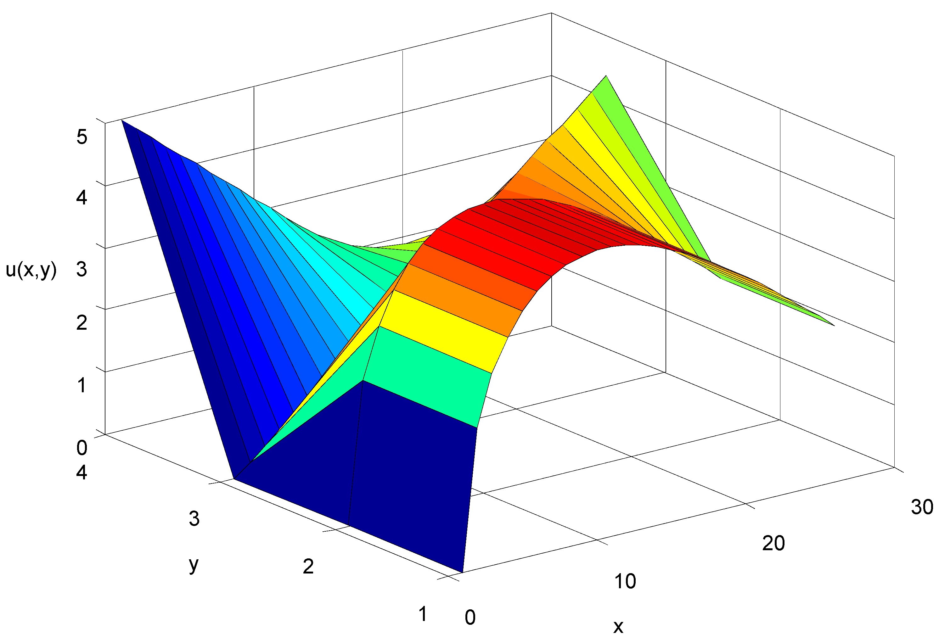
Figure 2.
The plot of the solution to the local fractional Helmholtz equation with fractional order α = ln(2)/ln(3).
Figure 2.
The plot of the solution to the local fractional Helmholtz equation with fractional order α = ln(2)/ln(3).

Figure 3.
The plot of the solution to the local fractional Helmholtz equation with fractional order α = 1.
Figure 3.
The plot of the solution to the local fractional Helmholtz equation with fractional order α = 1.
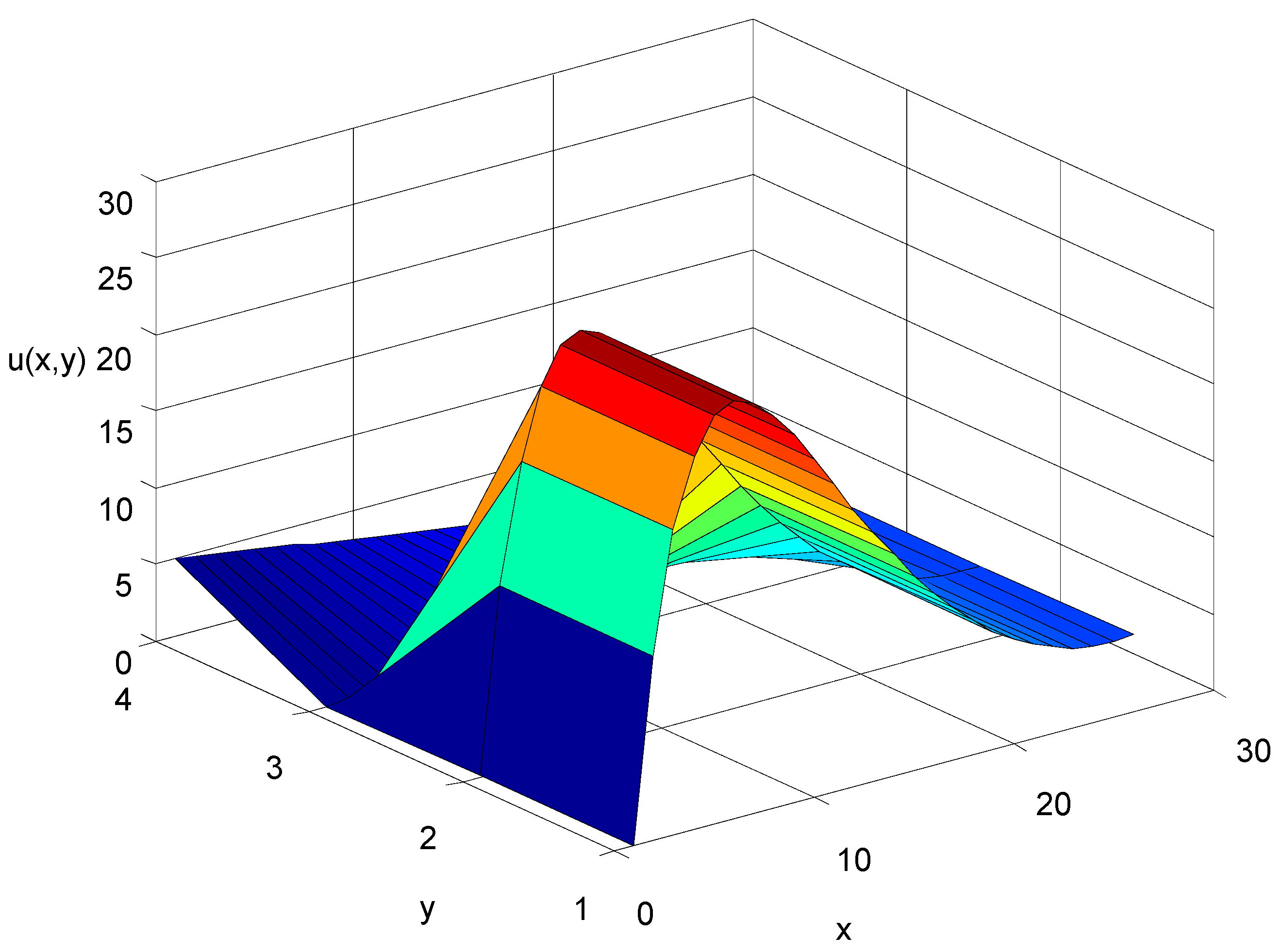
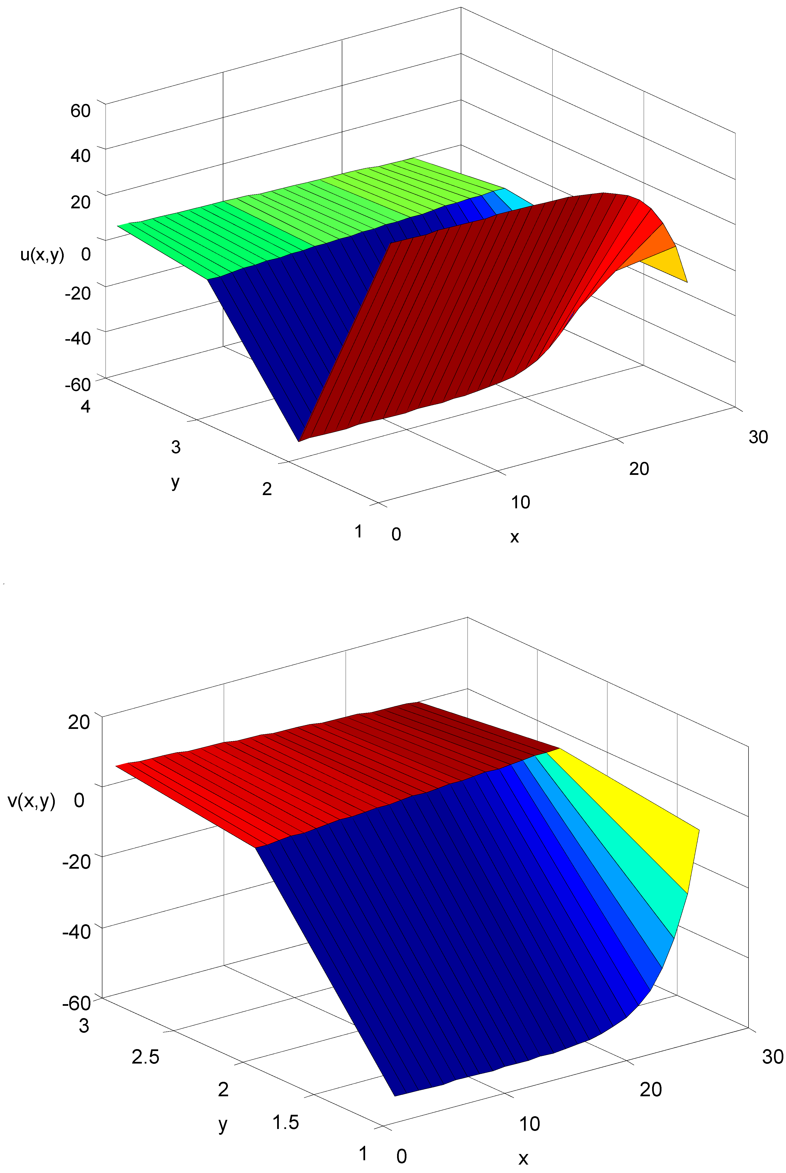
Figure 4.
The plot of the solutions to the coupled Helmholtz equations involving the local fractional derivative operator with fractional order α = 1/2.
Figure 4.
The plot of the solutions to the coupled Helmholtz equations involving the local fractional derivative operator with fractional order α = 1/2.
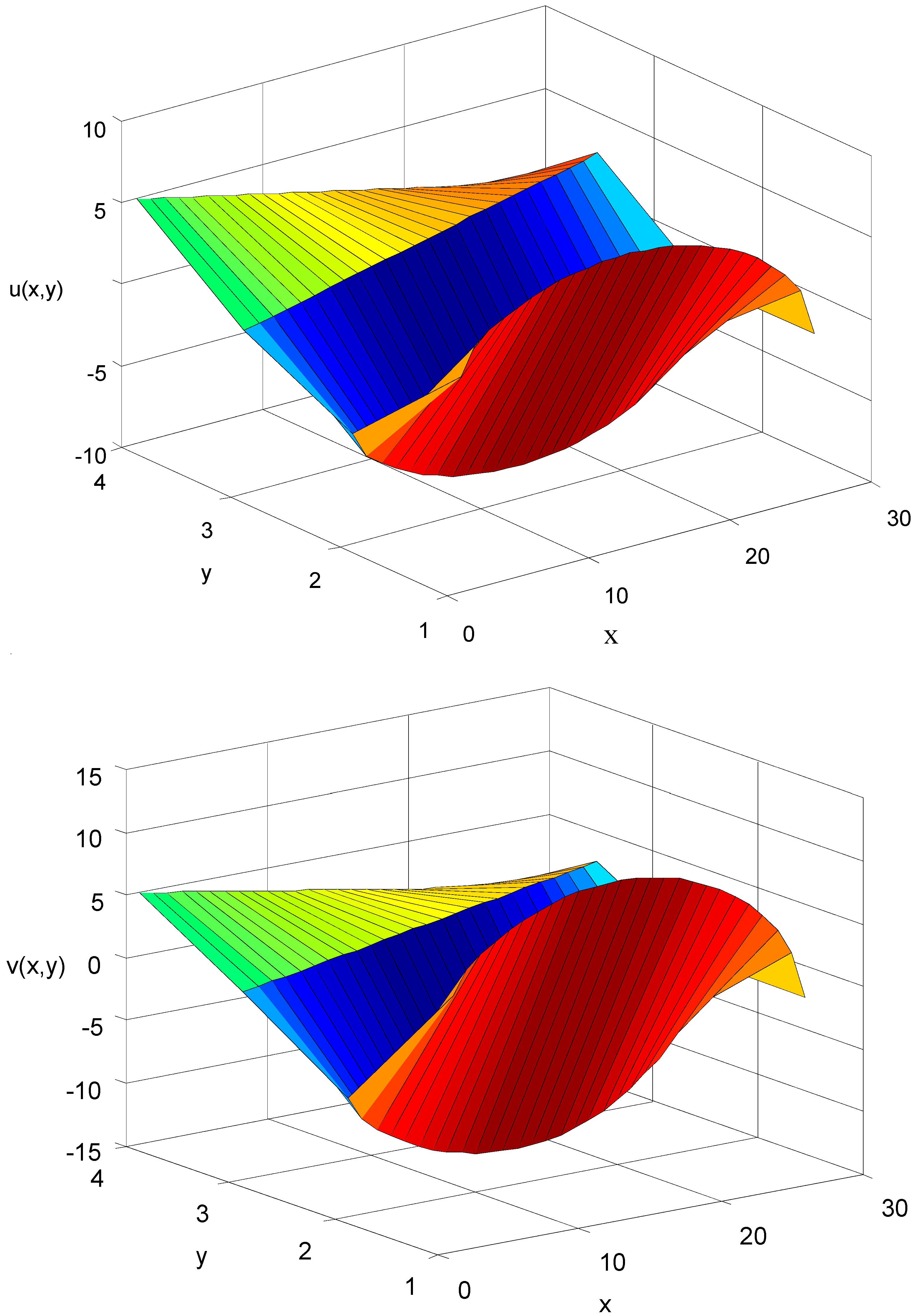
Figure 5.
The plot of the solutions to the coupled Helmholtz equations involving the local fractional derivative operator with fractional order α = 1.
Figure 5.
The plot of the solutions to the coupled Helmholtz equations involving the local fractional derivative operator with fractional order α = 1.

© 2019 by the authors. Licensee MDPI, Basel, Switzerland. This article is an open access article distributed under the terms and conditions of the Creative Commons Attribution (CC BY) license (http://creativecommons.org/licenses/by/4.0/).
Share and Cite
MDPI and ACS Style
Baleanu, D.; Jassim, H.K.; Al Qurashi, M. Solving Helmholtz Equation with Local Fractional Derivative Operators. Fractal Fract. 2019, 3, 43. https://doi.org/10.3390/fractalfract3030043
AMA Style
Baleanu D, Jassim HK, Al Qurashi M. Solving Helmholtz Equation with Local Fractional Derivative Operators. Fractal and Fractional. 2019; 3(3):43. https://doi.org/10.3390/fractalfract3030043
Chicago/Turabian StyleBaleanu, Dumitru, Hassan Kamil Jassim, and Maysaa Al Qurashi. 2019. "Solving Helmholtz Equation with Local Fractional Derivative Operators" Fractal and Fractional 3, no. 3: 43. https://doi.org/10.3390/fractalfract3030043