Regularized Integral Representations of the Reciprocal Gamma Function


1
Environment, Health and Safety, IMEC, 3001 Leuven, Belgium
2
Neuroscience Research Flanders, 3001 Leuven, Belgium
Fractal Fract. 2019, 3(1), 1; https://doi.org/10.3390/fractalfract3010001
Submission received: 16 November 2018
/
Revised: 29 December 2018
/
Accepted: 8 January 2019
/
Published: 12 January 2019
(This article belongs to the Special Issue The Craft of Fractional Modelling in Science and Engineering 2018)
Abstract
:This paper establishes a real integral representation of the reciprocal Gamma function in terms of a regularized hypersingular integral along the real line. A regularized complex representation along the Hankel path is derived. The equivalence with the Heine’s complex representation is demonstrated. For both real and complex integrals, the regularized representation can be expressed in terms of the two-parameter Mittag-Leffler function. Reference numerical implementations in the Computer Algebra System Maxima are provided.
MSC:
33B15; 65D20; 30D101. Introduction
Applications of the Gamma function in fractional calculus and the special function theory are ubiquitous. For example, the function is indispensable in the theory of Laplace transforms. The history of the Gamma function is surveyed in [1], in which the author further states that “of the so-called ’higher mathematical functions’, the Gamma function is undoubtedly the most fundamental”. A classical reference on the Gamma function is given by Artin [2]. The Gamma function has numerous remarkable properties that are surveyed in [3]. For example, one of its classical applications is the formula for the volume of an n-dimensional ball.
The reciprocal Gamma function is a normalization constant in all of the classical fractional derivative operators: the Riemann–Liouville, Caputo, and Grünwald–Letnikov. The reciprocal Gamma function is also prominent in the analytic number theory and its various connections to other transcendental functions (for example, the Riemann zeta function). Therefore, methods for the fast computation of the reciprocal Gamma function for arbitrary arguments may be beneficial for numerical applications of fractional calculus.
In the special function theory, the Gamma function is used explicitly in the definitions of the Fox type and Fox–Wright type of special functions, which are related to actions of fractional differential operators [4].
In a previous work, I investigated an approach to regularize derivatives at points where the ordinary limit diverges [5]. This paper exploits the same approach for the purposes of numerical computation of singular integrals, such as the Euler integrals for negative arguments.
The present paper proves a real singular integral representation of the reciprocal function. The algorithm was implemented in the computer algebra system Maxima for reference and demonstration purposes.
As a second application, the paper provides an integral representation of the Gamma function for negative numbers related to the Cauchy–Saalschütz integral [6]. The algorithm was also implemented in Maxima. Finally, the paper demonstrates an equivalent regularized complex representation based on the regularization of the Heine integral. The regularization procedure can be expressed in terms of the two-parameter Mittag-Leffler function.
2. Preliminaries and Notation
The reciprocal Gamma function is an entire function. Starting from the Euler’s infinite product definition, the reciprocal Gamma function can be defined by the infinite product:
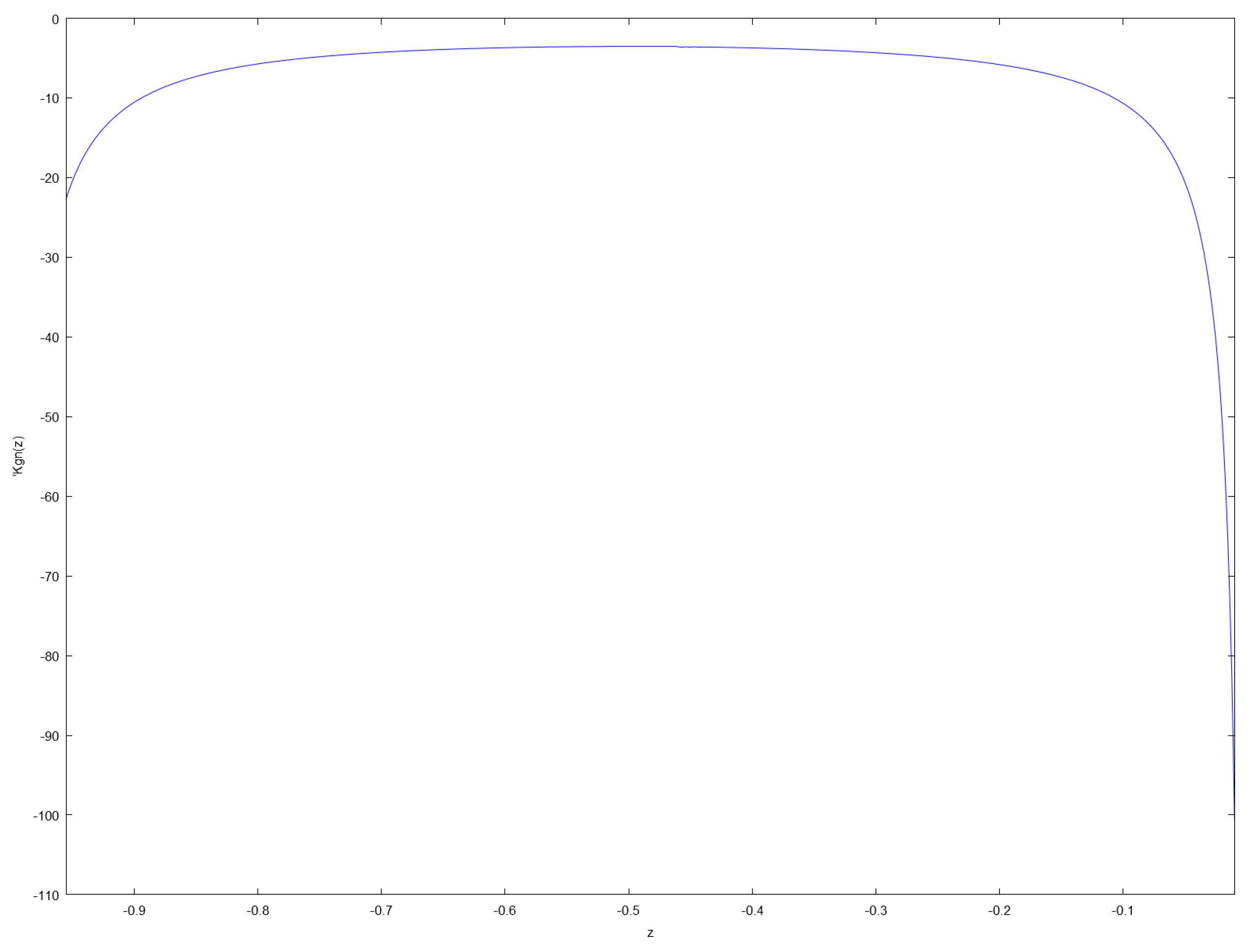
Proceeding from the Euler’s reflection formula for negative arguments, the reciprocal Gamma function is simply
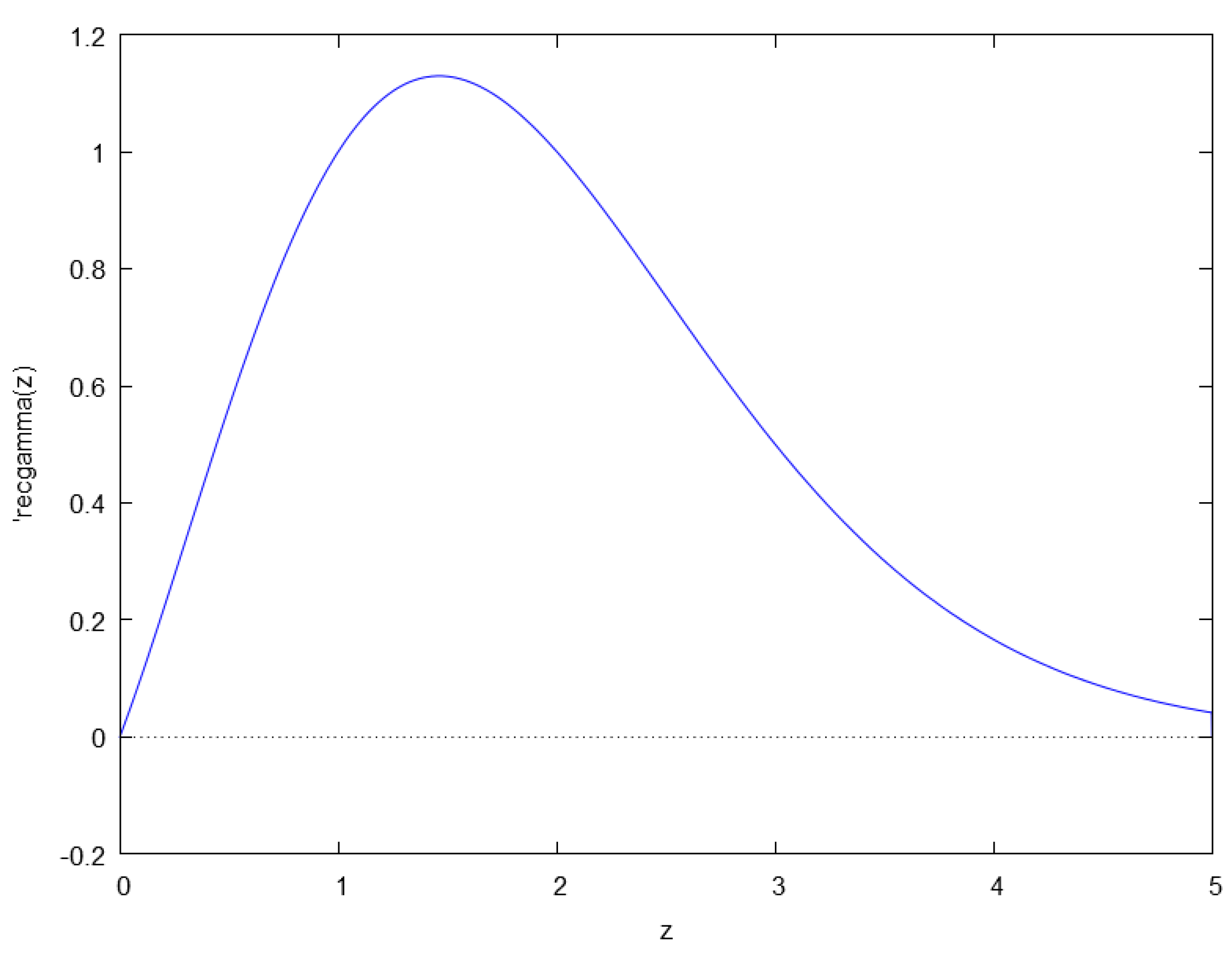
The plot of the above function is presented in Figure 1.
2.1. Real Representations
The Euler’s Gamma function integral representation is valid for real or complex numbers such that
However, for negative z, the integral diverges. A less well-known integral representation for is the Cauchy–Saalschütz integral [7] (Chapter 3), also along the real line:
where is given by Definition 3.
2.2. Complex Representations
Hankel’s representation of the Gamma function is given as
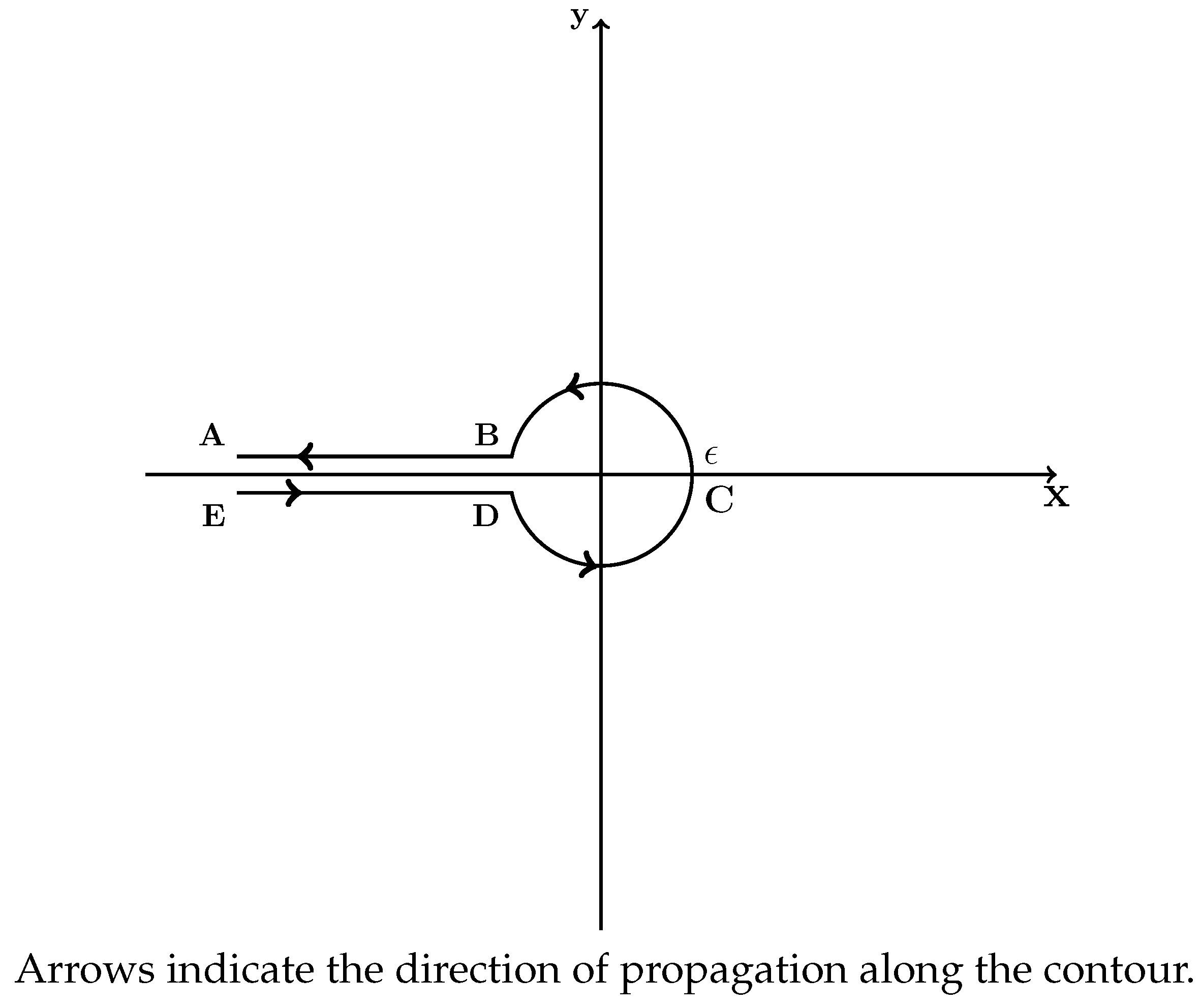
Here, denotes the Hankel contour in the complex -plane with a cut along the negative real semi-axis and circulation in the positive direction. The contour is depicted in Figure 2.
The Heine’s complex representation of the reciprocal Gamma function is well known and is given below [6] (p. 161):
is the reflection of across the origin. The integrand has a simple pole at . The Hölder exponent at 0 can be computed in the closed interval as
Therefore, for , it holds that and the order of the residue is the integer part . This observation is indicative of the statement of the main result of the paper.
2.3. Auxiliary Notation
Definition 1.
For a real number z, the notation will mean the integral part of the number, while will denote the non-integral remaining part.
Definition 2.
The falling factorial is defined as
Definition 3.
Let
be the truncated Taylor polynomial under the convention .
3. Theoretical Results
Theorem 1 (Real Reciprocal Gamma Representation).
Let , and . Then
where the integrals are over the real axis.
Proof.
First, we establish two preliminary results. Consider the following limit of the form and apply n times l’Hôpital’s rule:
Another application of l’Hôpital’s rule leads to
Therefore,
Secondly, consider the limit
Therefore,
Therefore, in order for both limits to vanish simultaneously, . Therefore, . Let .
In the following, we take as its principal value. Then,
by the above results. Therefore, by reduction,
Therefore,
by Euler’s reflection formula. We take the imaginary part of the integral, since is real and the middle expression is imaginary. Therefore,
Therefore,
Finally, by change of variables ,
□
Corollary 1.
By change of variables, it holds that
The latter result can be useful for computations with large arguments of .
Corollary 2 (Modified Euler Integral of the Second Kind).
By change of variables, it holds that, for ,
Finally, it is instructive to demonstrate the correspondence between the complex-analytical representation and the hypersingular representation.
Theorem 2 (Regularized Complex Reciprocal Gamma Representation).
For , and ,
where .
Proof.
The proof technique follows [8]. We evaluate the line integral along the Hankel contour:
with kernel
The contour is depicted in Figure 2. The integral can be split into three parts,
along the rays AB, DE, and the arc BCD, respectively. Along the ray AB, where , the kernel becomes
Along the ray DE, where , the kernel becomes
Therefore, changing the direction of DE, the rays can be added as
For
Therefore,
by Azrelá’s theorem.
The integral on the (closure of the) arc BCD is given by the Cauchy Residue Theorem. By the above observation, the residue at is given by the limit
since . Therefore, in the limit where the arc closes to a circle,
Furthermore, after integration by parts,
since . Therefore, the claim follows by reduction to □.
Remark 1.
These results demonstrate that the regularized complex contour integral can be collapsed to an integral along the real line. The same principle can be used for the regularization of other nonlinear functions; for example, the Beta function or the Wright function [8].
It is interesting to note a connection to the Mittag-Leffler function.
Definition 4 (Mittag-Leffler function).
The two-parameter Mittag-Leffler function [9] under the present convention is denoted by
Notably, the regularizing kernel can be expressed in terms of the two-parameter Mittag-Leffler function of integer arguments. The basis for the computation is the following auxiliary result:
Proposition 1.
Proof.
By direct computation,
□
Therefore, it directly follows that
Corollary 3.
For , and ,
where and in the last integral.
In a similar way, for an integer argument n, we have
Corollary 4.
For
where the circulation of the contour is counterclockwise around the origin.
Proof.
The computation follows from the Cauchy formula for derivatives:
Therefore, for and substitution ,
For , let . The integrand has the form . Therefore, in limit
Finally, we observe that
□
4. Applications
4.1. Laplace Transform Pairs
Consider the Laplace transform . As a concrete application of Theorem 2, consider the pair
The inverse Laplace transform can be calculated simply as
by change of variables. The latter result can be used for numerical inversion of Laplace transforms.
4.2. Ratios of Gamma Functions
Secondly, the ratio of two Gamma functions can be represented as
Proposition 2.
Let . Then,
where .
Proof.
□
4.3. The Cauchy–Saalschütz Integral
Finally, for negative arguments:
Proposition 3.
For , it holds that
Proof.
By the reflection formula,
Therefore,
□
4.4. The Grünwald–Letnikov Derivative
The Grünwald–Letnikov derivative is defined [10] as
For numerical applications, the limit is approximated as the finite difference for some large . Therefore, Theorem 1 can be directly applied to compute the approximation for small m. For large m, on the other hand, the Stirling asymptotic formula can be used. Pursuing such application, however, goes beyond the scope of the present paper.
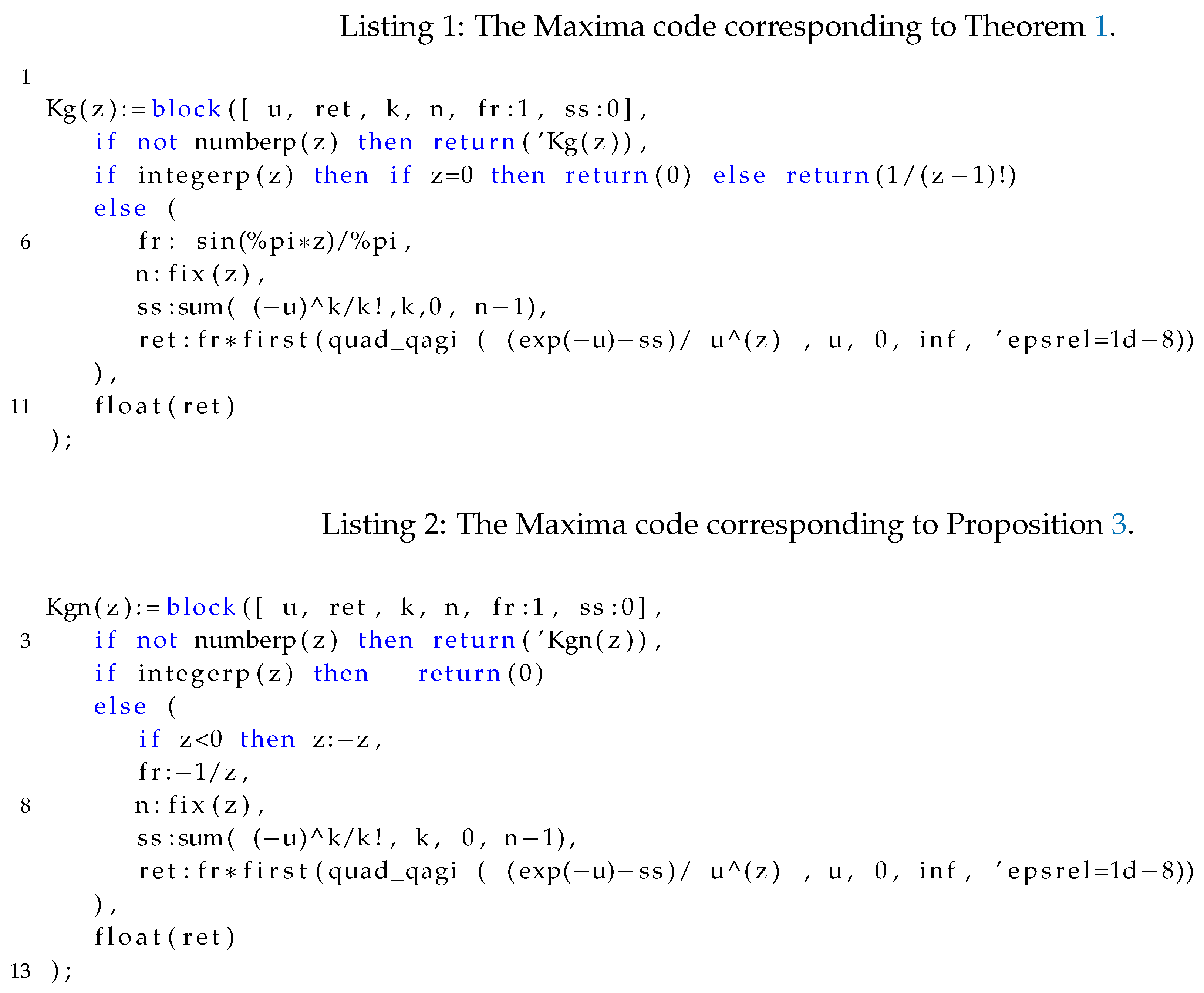
5. Numerical Implementation
A reference implementation in the computer algebra system Maxima is given in Listings 1 and 2. The numerical integration code uses the library Quadpack, distributed with Maxima. The reference implementation given in this section uses a routine for semi-infinite interval integration with a tunable relative error of approximation (i.e., the epsrel parameter). A plot of the reciprocal function computed from Listing 1 is presented in Figure 3.
Figure 4 represents a plot of computed from Listing 1.
Acknowledgments
The work has been supported in part by grants from Research Fund—Flanders (FWO), contract number VS.097.16N, and the COST Association Action CA16212 INDEPTH. Plots were prepared with the computer algebra system Maxima.
Conflicts of Interest
The author declares no conflict of interest.
References
- Davis, P.J. Leonhard Euler’s integral: A historical profile of the Gamma function: In memoriam: Milton Abramowitz. Am. Math. Mon. 1959, 66, 849–869. [Google Scholar] [CrossRef]
- Artin, E. The Gamma Function; Holt, Reinhart and Winston: New York, NY, USA, 1964. [Google Scholar]
- Borwein, J.M.; Corless, R.M. Gamma and factorial in the monthly. Am. Math. Mon. 2018, 125, 400–424. [Google Scholar] [CrossRef]
- Kiryakova, V. All the special functions are fractional differintegrals of elementary functions. J. Phys. A Math. Gen. 1997, 30, 5085–5103. [Google Scholar] [CrossRef]
- Prodanov, D. Regularization of derivatives on non-differentiable points. J. Phys. Conf. Ser. 2016, 701, 012031. [Google Scholar] [CrossRef] [Green Version]
- Mainardi, F. Fractional Calculus and Waves in Linear Viscoelasticity; Imperial College Press: London, UK, 2010. [Google Scholar]
- Temme, N. Special Functions; John Wiley & Sons: New York, NY, USA, 1996. [Google Scholar]
- Luchko, Y. Algorithms for evaluation of the Wright function for the real arguments’ values. Fract. Calc. Appl. Anal. 2008, 11, 57–75. [Google Scholar]
- Mittag-Leffler, G.M. Sur la nouvelle fonction Ea(x). C. R. Acad. Sci. Paris 1903, 137, 554–558. [Google Scholar]
- Oldham, K.B.; Spanier, J.S. The Fractional Calculus: Theory and Applications of Differentiation and Integration to Arbitrary Order; Academic Press: New York, NY, USA, 1974. [Google Scholar]
Figure 1.
computed from Equation (1).
Figure 1.
computed from Equation (1).
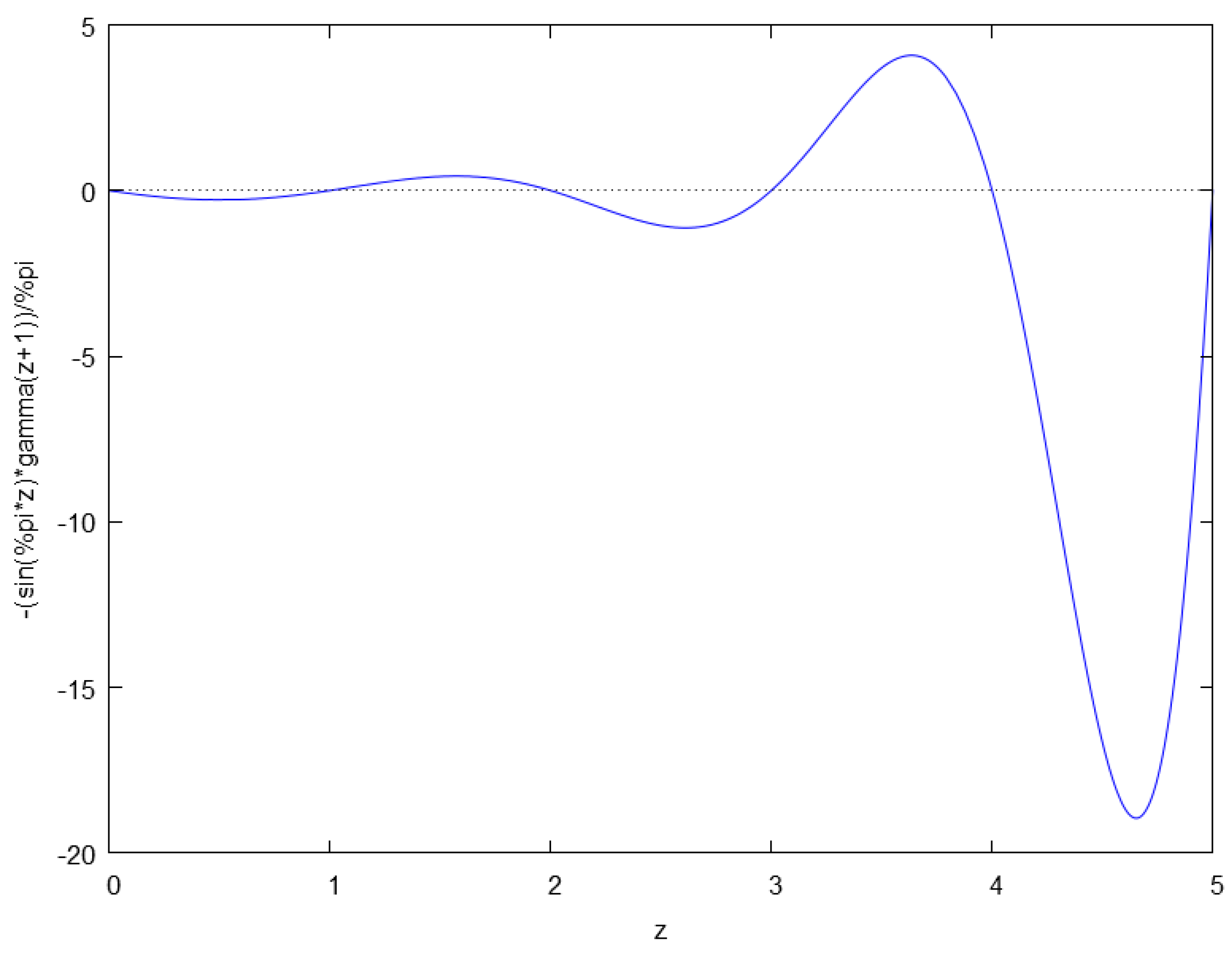
Figure 2.
The Hankel contour .

Figure 3.
computed from Theorem 1.

Figure 4.
computed from Proposition 3.
© 2019 by the author. Licensee MDPI, Basel, Switzerland. This article is an open access article distributed under the terms and conditions of the Creative Commons Attribution (CC BY) license (http://creativecommons.org/licenses/by/4.0/).
Share and Cite
MDPI and ACS Style
Prodanov, D. Regularized Integral Representations of the Reciprocal Gamma Function. Fractal Fract. 2019, 3, 1. https://doi.org/10.3390/fractalfract3010001
AMA Style
Prodanov D. Regularized Integral Representations of the Reciprocal Gamma Function. Fractal and Fractional. 2019; 3(1):1. https://doi.org/10.3390/fractalfract3010001
Chicago/Turabian StyleProdanov, Dimiter. 2019. "Regularized Integral Representations of the Reciprocal Gamma Function" Fractal and Fractional 3, no. 1: 1. https://doi.org/10.3390/fractalfract3010001