A Traffic Analysis on Serverless Computing Based on the Example of a File Upload Stream on AWS Lambda


1
School of Computing, Edinburgh Napier University, Edinburgh EH10 5DT, UK
2
Eight Bells LTD, Nicosia 2002, Cyprus
*
Authors to whom correspondence should be addressed.
Big Data Cogn. Comput. 2020, 4(4), 38; https://doi.org/10.3390/bdcc4040038
Submission received: 29 October 2020
/
Revised: 1 December 2020
/
Accepted: 7 December 2020
/
Published: 10 December 2020
Abstract
:The shift towards microservisation which can be observed in recent developments of the cloud landscape for applications has led towards the emergence of the Function as a Service (FaaS) concept, also called Serverless. This term describes the event-driven, reactive programming paradigm of functional components in container instances, which are scaled, deployed, executed and billed by the cloud provider on demand. However, increasing reports of issues of Serverless services have shown significant obscurity regarding its reliability. In particular, developers and especially system administrators struggle with latency compliance. In this paper, following a systematic literature review, the performance indicators influencing traffic and the effective delivery of the provider’s underlying infrastructure are determined by carrying out empirical measurements based on the example of a File Upload Stream on Amazon’s Web Service Cloud. This popular example was used as an experimental baseline in this study, based on different incoming request rates. Different parameters were used to monitor and evaluate changes through the function’s logs. It has been found that the so-called Cold-Start, meaning the time to provide a new instance, can increase the Round-Trip-Time by 15%, on average. Cold-Start happens after an instance has not been called for around 15 min, or after around 2 h have passed, which marks the end of the instance’s lifetime. The research shows how the numbers have changed in comparison to earlier related work, as Serverless is a fast-growing field of development. Furthermore, emphasis is given towards future research to improve the technology, algorithms, and support for developers.
1. Introduction
The development of Cloud Computing is at the forefront of centralising application development and management, with a considerable impact on their configuration(s). It enables developers to use computer resources as a service, and therefore facilitates scaling application and access to data from anywhere, while saving costs and keeping hardware maintenance at low levels [1]. To keep up with the rapid development of the underlying technology, more and more companies are shifting their Information Technology (IT) infrastructures to the cloud, while providers offer more services in return. The shift towards microservices, Virtual Machines (VM) and advanced individual operating systems running in containers, make it possible to share hardware, thus saving a significant amount of resources. Services can now be rapidly spun up through server-oriented repackaging of UNIX processes and namespace virtualisation without a large overhead of hardware configuration. Additionally, responsibilities are shared and performance increases drastically through the wider usage of advanced load balancing algorithms.
A Serverless architecture takes this evolution one step further and has been drawing increasing attention, according to Google search trends [2]. The traditional programming paradigm follows the concept of composing functions, which map inputs to outputs, into programs which are now outsourced to the cloud. In the background, a working service handles public requests, typically from Application Programming Interfaces (APIs), through managing and executing function containers. With AWS Lambda, the largest public cloud provider, AWS, has launched a major innovation for developers, which was first introduced in 2014 [3]. Through the concept of Function as a Service, applications are decomposed into lightweight, stateless functions that perform actions and are triggered by simple events on demand [4]. This may be a user update, such as an image upload that triggers the function through a REST service to place that image and its metadata in the data store [5]. Providers promise new capabilities to make scalable microservices more approachable and cost-effective, as they focus on charging for execution time rather than resource allocation. The idea is that clients need only consider their business set-up, and leave any server configurations to the responsibility of the provider.
The Gartner Technology Report [6] stated in 2016 that the value of Serverless computing has been clearly demonstrated, as it maps naturally to a microservice software architecture, while being on a trajectory of increased growth and adoption. However, technological development has become a commercial focus and thus research is largely in the hands of the individual provider. Unfortunately, much of that information is not provided to the public and thus practices exhibit some degree of obscurity, an issue that academia ideally needs to address by providing better support for practitioners. As web traffic is increasing on a steady basis, where small services contribute even more, it is important to locate bottlenecks, show hidden problems and optimise resource allocation on an application level.
Following the call of academia [7,8,9] for monitoring the obscure environment surrounding Serverless architectures and using the data to update and better cater for uncertainties, our work aims to present an overview of the configuration architecture concerning auto-scaling and effective load-balancing of traffic on Serverless environments. After an initial introduction to the topic and the problems providers and clients face, a research approach is taken to investigate how Serverless traffic is achieved in the case of the most popular Serverless provider, AWS Lambda. Our work examines performance such as the response time and different functions states with respect to the underlying VM. The performance analysis based on an example AWS S3 File Upload handler could provide input for designing such applications by giving insight into the advantages and possible problems. The results can potentially support Serverless users with application performance, service level agreements (SLAs) and security concerns. The contributions of our work can be summarised as follows:
- We examine the process flow, thus optimising the resource allocation facing the provider’s trade-off between resource and cost savings, and provisioning latency for Serverless environments.
- We identify factors influencing traffic and resulting performance (execution time, high demand resistance), to understand instance-launching, auto-scaling and load-balancing on function invocation events, based on various experimental settings.
- We evaluate auto-scaling and effective load balancing of traffic, as carried out by AWS on AWS Lambda.
The rest of the paper is organised as follows. Section 2 includes the literature review and related work. Section 3 describes the experimental test set-ups used to investigate traffic performance and scaling processes on AWS Lambda. Section 4 provides our experimental results. Section 5 concludes the paper and provides pointers for future work.
2. Literature Review and Related Work
The growing need for a shared network of nodes, fast response rates of services, the resulting agility of resource provisioning, and minimised management during run-time have been targets of hyper-scaling microservice platforms in recent years [2,10]. This refers to the pooling and utilising of resources including operating systems, runtime environments and hardware on a pay-on-demand basis [10]. The main concept behind this is called microservisation. It entails the creation of business functionalities as small running services that interact through standardised interfaces, such as REST APIs. The concept aims to facilitate flexibility to cope with the operation, maintenance and traffic-management providing a more cost-effective quality of service [11].
The development of Serverless architectures originates from the need for more focused peer-to-peer software and client-side-only solutions. Serverless functions offer the possibility to act as a simple and quick service in response to events such as new files being uploaded to a cloud data store, messages arriving in queue systems, or even direct HTTP calls. As they are executed in the provider’s environment, it works well for linked nodes [5]. The approach frees the user from having to maintain a server, including configuration and management of VMs, as resource management is fully provided by the platform in an automated and scalable way. Billing is promised to be limited to the actual volume of resources consumed [10]. The difference between Platform as a Service and Serverless is that the latter not only scales on-demand but also runs on-demand, as providers enable instances to go cold. This shifts the runtime concerns to the provider and leaves the developer needing only to consider the programming model [10,12]. Balancing the right size and number of services should be the only architectural concept the developer has to think about. Decomposing the application’s landscape into smaller units may influence functional requirements, so the architecture depends on the level of granularity [4,13]. This is why a Serverless solution is preferred for Greenfield rather than Brownfield development [11,14]. Small functions naturally fit the growing use of microservices. With short run times, this allows the provider to maintain low costs and to use it to fill the load between larger jobs on the cloud [12]. Busy, low-duty and low-maintenance applications such as algorithms for information access and data transformation serve as good examples. This includes for example algorithms for a file upload stream, or music recognition [2,15]. Long-running, stateful and CPU-intense services such as deep learning or stream analysis on the other hand are not yet suitable [12,14].
In a Serverless architecture, a significant part of the flow performance depends on the network itself [16]. A persistently low throughput indicated by high latency hints a bottleneck located in the network, so it is important to re-arrange the architecture continuously. It is up to the provider to terminate uneconomical groups and set best practice rules. As more autonomy is given to the service provider, it is important to replicate the tractability of the architecture, specifically the design of the underlying infrastructure, ensuring the optimal level of resource allocation. This includes monitoring function initialisation requests; the number of running containers, active VMs and the deployment, as well as scaling of traffic across clusters [17].
As AWS Lambda is most-used and associated with the most popular Serverless platform, it is taken as the base platform for research [2,10]. Most studies are based on the configuration and performance of containers and VMs in general. As shown in the previous section, the same concepts apply for Serverless. However, there are additional factors influencing traffic allocation in such environments, as providers need to meet the trade-offs of SLAs while minimising their costs. Hendrickson [18], for example, measured request latency on AWS Lambda and discovered it had higher latency than AWS Elastic Beanstalk, the AWS Platform-as-a-Service orchestration system. Lloyd [19] investigated those factors affecting application performance in AWS and developed a heuristic to identify which VM a function runs on based on the VM uptime in the UNIX /proc/stat directory [19]. Using the underlying Linux process to gather information has been found to be the most common tool to overcome the obscurity of AWS. In their study, this has been achieved through reassembling the Lambda environment of 512 MB with a Docker Container. Their results indicate that the average uptime of a VM is 2 h, and these have distinct boot times. In addition, the standard deviation for load balancing observed on the Docker engine indicates discontinuity, as it is increasing and therefore stresses some nodes in the network. They show that high memory stress causes the code execution to slow down and thus increases latency, as more containers need to be launched. A cold VM increases latency by an average of 15 s, and containers go cold after an average of 10 min idle time. However, their results lack evidence of the actual AWS architecture and therefore need to be evaluated with caution.
Wang [9] performed a major study on the design of Serverless Platforms in 2018 and presented their results at the 2018 USENIX Annual Technical Conference. Following prior discussion of studies on load balancing, their study aimed to discover the design pattern for handling low duty-cycle workloads as changes in the Linux files stored. To re-construct the architecture, they made use of the fact that every function instance is represented on a local disk for temporal data storage, to wit the proc file system on Linux (procfs). This can be accessed to monitor the activity of co-resident instances in the Serverless environment. Their methodology follows a code framework that defines functions to perform relevant investigation tasks, such as collecting invocation timing, instance runtime information and subroutines. In their experiments, they conducted a number of invocations of the same number of concurrently running function instances on AWS. In this way, the procfs file system exposes global statistics of the underlying VM host, such as profiling runtimes and identifying the IPs used on a larger scale. However, in contrast to Lloyd’s findings, they determined that the results of their methodology do not indicate the same boot time for VMs as assumed. They also indicated a much longer idle time of 37 min, which is up for further discussion when considering experimentation in Section 4.
Their results further show that AWS Lambda achieves the best performance in scalability and Cold-Start latency, compared to the other two major providers, Google Cloud and Microsoft Azure. They claimed the reason is that AWS uses a pool of ready VMs and manages launching and scheduling modules through a CPU bin-packing algorithm. The findings were also confirmed by McGrath and Brenner [7]. With more CPU power, the environment set becomes faster. It must, therefore, be allocated proportionally with memory size, which is confirmed in the AWS Lambda Documentation [4]. This means the algorithm places a new function instance on an existing active VM to maximise VM memory utilisation rates. In terms of latency, it has been found that function memory and choice of languages can be a bottleneck on AWS, highlighting the need for a more sophisticated loading mechanism. Furthermore, instances with higher memory demand get more CPU cycles, but the instances share the CPU fairly.
Researchers are raising concerns for security issues, regarding the use of IAM (Identity and Access Management) roles [9] to isolate the function instances of multi-account applications from different application accounts. Since they share the same VMs, this creates a single point of failure in the infrastructure. Wang [9] recommended AWS allocate sets of VMs to IAM roles rather than accounts. With a successful experiment, their work also discovered the vulnerability in the procfs system, as it can be used for attacks. Limited accesses to runtime information should, therefore, be included as a major SLA. Nevertheless, they argued that providers should expose such information in an auditable way for their clients. Through accessible information, for example from an API call, clients would be able to detect and block suspicious behaviour [9].
A more sophisticated study of a special service was conducted by McGrath and Brenner [7], which implemented a prototype that can be used as an example use-case for an API communicating with data storage through a Serverless function. Their results show a performance drop after 14 concurrent requests, despite the maximum concurrency level on AWS officially being 200 [4]. Further investigation showed that the latency increase is caused by the storage system warm queue, highlighting the requirement to monitor the status of active executions to re-execute and re-provision in such cases. Consequently, throughput characteristics influence the performance of traffic drastically when numerous parallel running instances access the storage. Following this study specifically, research on another use-case was conducted by Pérez et al. [20]. They developed a system that pulls from a Docker container to deploy a specified image on Lambda to find a workaround for the stateful component, but they also reported throughput difficulties. Pelle [21] also used a measurement framework to capture delay characteristics and applied it to a latency-sensitive drone control application. Although they did not publish their methodology, their results may still serve for comparison. Our work differs from all previous approaches because it aims to investigate how the optimal balancing is achieved on AWS, thus providing details on what impact the load balancing may have on the client, and the importance of the request rate in AWS Lambda.
3. Methodology
As AWS is perceived as rather atomic and obscure for the practitioner, the focus of our work is to gain a proper understanding of the underlying infrastructure architecture. Through the collection of data from the underlying Linux system, it is possible to explain load balancing on AWS Lambda. We aim to answer the following questions: (a) How are the servers configured? (b) How is traffic distinguished? (c) What happens in the case of traffic increase? This particularly requires investigation of Cold-Start latency, instance-launching and the auto-scaling of host VMs. The experiments measure performance by the number of concurrent requests, execution duration and Round-Trip time, as well as the CPU and memory available, in light of resource limitations regarding request rates, execution time and contention of instances. As the AWS Lambda architecture enables instances to go cold and not run continuously as a dedicated machine, the code reacts to events delicately and scales out according to the request workload, which influences the behaviour of the application, as well as the consumption and billing plan [4].
The total time it takes to wait for a request fulfillment, from invoking a function after receiving the event until its return, is called latency. When a new instance needs to be launched, a Cold-Start will increase latency. It further increases Round-Trip time and execution duration and thus limits the performance of Serverless environments, and it is therefore subject to experimentation here. Fluctuating latency when scaling up could be a bottleneck for real-time-sensitive applications, especially those requiring concurrent invocations. In respect of the research questions, the results from the experiments may provide developers with runtime and monitoring support and information on AWS’s SLA fulfillment, as scalability and fault-tolerance of invocations have been identified as the customer’s main points of concern.
In particular, two sets of experiments have been carried out to gather such information. First, a general Lambda function measurement test was used, aiming to reverse-engineer the underlying resource management and architecture, including information on the processors and memory sizes. This is also tested on performance baselines such as language versions, memory sizes, contention and concurrency. A second experiment then aims to expand this on a larger scale to investigate traffic allocation such as the distribution of VM instances and their corresponding differences in IP addresses, depending on the incoming request rate. As AWS Cloud Watch monitors by default the number of requests, execution duration per request and memory used, the tool can be used as a starting point to analyse Lambda Logs for latency and execution mapping. The data from the logs are then extracted for further analysis. This includes for example descriptive statistics including pattern recognition as well as descriptions of the instance launching procedure depending on the request volume of the incoming traffic. As increasing traffic is associated with a tighter latency bound, the experiments aim to determine whether hosts are in a running state or not, and how AWS evenly distributes requests over these. To further support experimentation, an AWS Lambda file upload stream microservice has then been integrated into the measurement function, with the aim of introspecting the platform’s performance and infrastructure management further. As a widely used Serverless use-case, the file upload stream serves as a basic example which has been found feasible given the computing power necessary for the tests in compliance with the resources available in the free trial version of the service. As experimenting in the free trial period restricted us in terms of time and workload, we therefore decided to focus on one basic application in order to investigate it in depth, and thus provide a methodology that may be extended to other, more sophisticated use cases.
Following our focus on gathering information on AWS Lambda’s underlying hardware system and scaling procedure, a variety of experimental measurements was used. We define a Function Instance to be the container (or sandbox) running the code. As per the definition of Serverless, it is launched depending on request volume and has restricted resources. In the experiments, the following settings for an instance were specified (Table 1).
The maximum time-out of 300 ms was found to be sufficient, although AWS has recently increased it, making up to 900 ms possible. The majority of experiments were carried out with the smallest available memory size, 128 MB, as most test runs used even less memory. Python was chosen as the runtime language for reasons of compatibility with the supporting tools. In addition, Python has been shown to be in the low field compared to other languages when conducting previous experiments on latency, thus using the language mitigates possibilities of language overhead influencing the results. Furthermore, it is easier to include subprocesses and get metadata from underlying systems compared to other languages. With Node.js, Python is also the most used language on AWS Lambda [8].
The Cold-Start is associated with the booting process of a single VM (instance launching). To allocate a server with capacity, the runtime must start up a VM, increasing latency. Services and other start-up applications are executed after the reboot. In AWS, this happens when a new instance handles its request after the initial deployment, and results in increasing the response time.
AWS documents [22] indicate the existence of a pool of idle VMs, which has been preconfigured with the runtime to limit Cold-Start latency. A Cold-Start of the VM (VM Cold) therefore does not form a part of the calculation. The Round-Trip time is an additional key performance indicator, as the execution duration and connection set-up time for packet delivery is limited in a Serverless environment.
The theoretical background indicates that, after the function instance is initially launched, it stays active for additional events. However, if it has not returned a response from the previous requests yet, another instance is launched to process concurrent requests. The routing of the requests to running or new instances is called auto-scaling. Subsequently, instances are terminated and may become idle after no new invocation requests are received.
Auto-Scaling can mainly be identified through monitoring IP address and instance ID changes. Both Cold-Start latency and auto-scaling are the key indicators of performance when investigating resource allocation when addressing the research questions. With the proposed experimental methodology, information regarding processes as they occur at function invocations is collected to establish the type of VMs the instances are run on, their timing and the distribution of the request traffic among them.
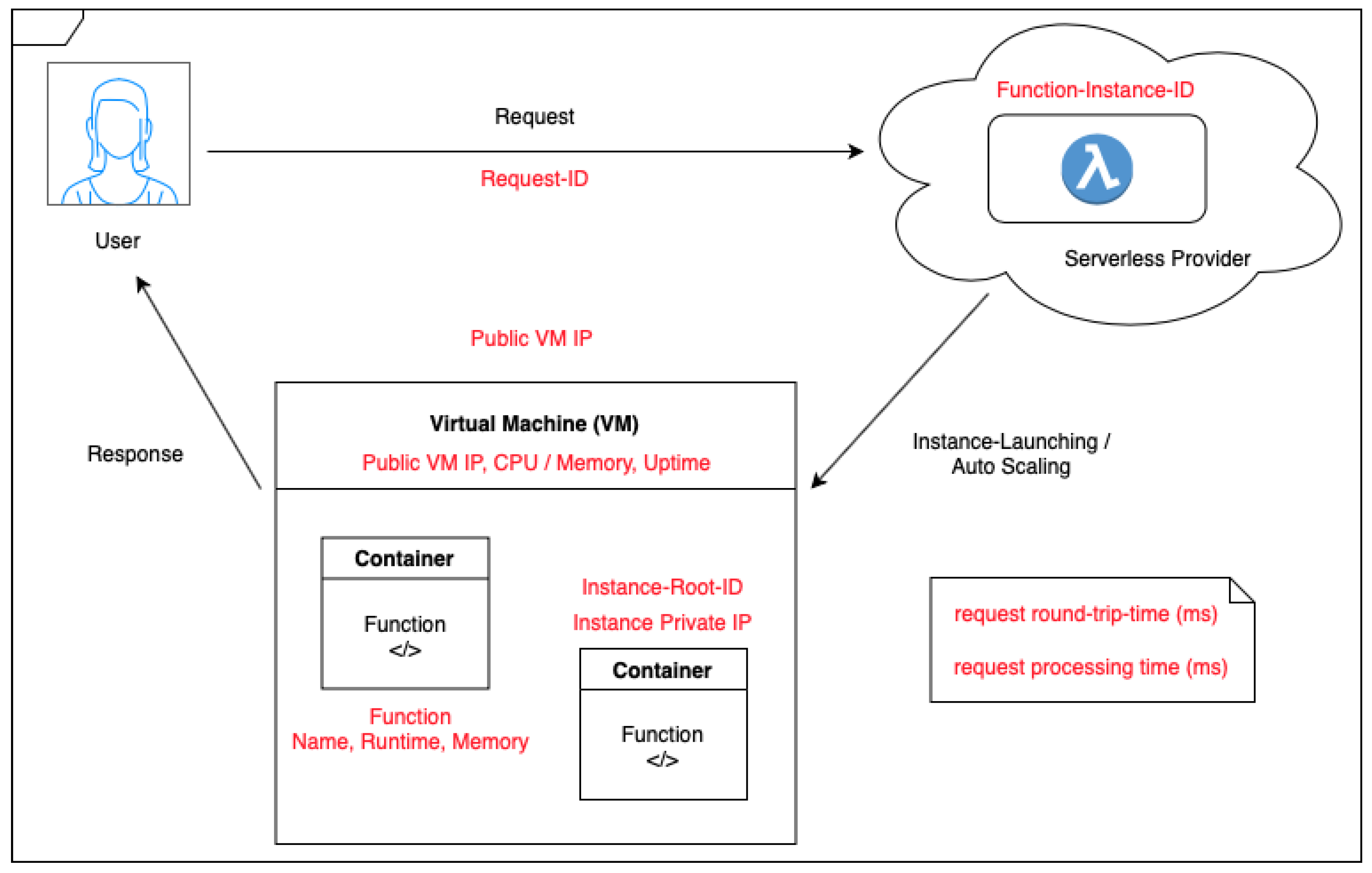
To sum up, Figure 1 illustrates an overview of the scaling process and the data gathered per request during experiments.
4. Results
The literature provides evidence of auto-scaling practices that can be tested during the experimentation. This includes the determination of key performance indicators such as latency, including Cold-Start and Round-Trip time. AWS’s (floating) IP design system could be useful for the load-balancing investigation, as such information could be taken from the underlying Linux procfs filesystem. However, given that access to run-time information is a security issue, the feasibility of the approach must first be tested. If successful, the filesystem will furthermore provide information on the underlying architecture, including the processor set-up. This way, it will be possible to gather further information on workload allocation on the VMs at traffic peak events, as recommended in the literature. It is also valuable to apply an accurate invocation event to the function instance to trigger the action through a web request and measure the influence of such timing compared to a direct invocation, a point which has often been missed.
This section summarises the presentation and comparison of the methodologies used and leads towards a discussion of the results and eventual differences. The findings are compared to previous findings in related academic work. A summary of the main findings can be found at the end of the section.
The goals of the evaluation are as follows:
- Measure performance characteristics of the execution environment
- Evaluate AWS’ scaling practices
- Validate the feasibility of the approach
The following subsections analyse in detail the results of the experiments conducted. Both experiments served to target the factors identified in the theoretical background as influencing traffic, in order to meet the proposed objectives regarding the performance of the AWS Serverless environment. The variety of settings helps clarify the findings regarding the system architecture and the automation process of the provider under real-world circumstances. The data collected during experimentation inform further discussion of the research questions. The results from the Function Distribution Measurement taken from Wang [9] mainly serve to investigate the AWS Serverless backend infrastructure, and the factors identified as influencing traffic are compared to previous findings in related academic work. The Traffic Distribution Analysis is further used to examine load-balancing and auto-scaling based on the previous findings and provide insight to support to developers. Similarities and differences between the findings of the experiments are also discussed.
To make the data accessible, the .log file resulting from the measurement framework was converted to a .csv to load it into the R Studio software (https://rstudio.com). For the Traffic Distribution Analysis, AWS CloudWatch logs were downloaded and imported with the .csv format directly. As AWS saves logs to Cloud Watch automatically, there is no need to implement a database when calling the API, as CloudWatch Insight serves as such. A successful request message can be identified and monitored on CloudWatch, along with error messages. Cloud Watch Insight and the Cloud Watch Query Language can be used to execute general requests on the data, such as selecting periods and corresponding graphical visualisation to show overall trends. Additionally, a series of tests with R Studio was run in both cases to clean up the data for them to be useful for subsequent descriptive statistics. Most of the plots describing key latency indicators show the statistical median and standard deviation.
Architecture: The data here show a column indicating the VM processor and memory. In addition, unique instance and VM IDs/ IPs and public IPs can be identified and compared to investigate AWS’ Serverless infrastructure.
Cold-Start Latency: Latency in providing VMs with the container instances running the code has been identified as a main indicator of performance, and thus influences traffic. As the Measurement Framework calculates Cold-Starts and Round-Trip time based on the request- and response-time timestamps, basic descriptive statistics such as mean, median, standard deviation and coefficient of variation of the measurements can be used to determine and compare results for several variable settings. A Correlation Test can furthermore establish direct influences and patterns.
In the case of the Traffic Distribution Analysis, the execution time and duration must be used to estimate Cold-Start latency and performance. However, the exact time cannot be calculated. With Postman, which was conducted in a sub-experiment, it is possible to track the TCP stack implementation and thus help calculate a Cold-Start indicator based on the duration, Round-Trip time and request sending time. Furthermore, it was found that AWS Lambda logs a initDuration value summarising the amount of run time to load the function for an initial request by default. Thus, the initDuration is one Cold-Start influence and only appears when a new instance is launched.
Load-Balancing and Auto-Scaling: Auto-scaling practices are evaluated mainly through the graphical investigation of the IP address distribution on VMs and by time series analysis. Both serve the purpose of indicating patterns when the addresses change based on the set request rate. The overall packet flow is also accessed with the Postman test conducted.
4.1. Function Distribution Measurement
The first set of experiments determines results for the AWS Lambda backend infrastructure, and performance factors such as Cold-Start and Round-Trip time based on the framework as introduced by Wang [9]. The experiments ran successfully, meaning the framework is still usable. For all subsequent tests, the median, standard deviation (to measure the average departure from the mean) and the interquartile range (to indicate variability) were conducted with R Studio. In addition, to better indicate general trends, the mean was used in cases where there is confidence that data are less skewed, for example when comparing language versions. The results for the Cold-Start, Scaling, Placement and Consistency Test as described in the Experimentation Section are as follows.
4.1.1. Test Results
The Cold-Start Test run on the different Python Versions of 2.7, 3.6 and 3.7 results in 48 observations, which are equal to 48 requests on 24 contesting Lambda function instances, as each function was invoked twice. For each version, this accounts for four deployed functions for each chosen memory size, 128 and 3008 MB. Table 2 describes the results of the overall test.
Overall, 15.98% of the Round-Trip Time is due to the Cold-Start. The standard deviation, measuring the amount of variation, indicates that the Cold-Start varies around 700 ms about the mean. Between the largest and lowest measurement, a difference of around 1–2 s can be determined.
Figure 2 shows a boxplot of the measured Cold-Start and Round-Trip time for each version.
The difference between the Python versions (Table 3 and Table 4) means for the Cold-Start vary around 0.1–0.2 s, but for the Round-Trip time no significant change can be detected. However, the boxplot shows a strong low whisker for Python 3.7. Investigation of whether the average time may be lower with a larger dataset however is out of the scope of this paper.
By testing the unique function names with their corresponding instances and VM IDs and IPs, the resulting data indicate no warm-starts, as the instance IPs and IDs change with each invocation. That indicates that each instance is launched on a different VM.
File Upload Stream: The Cold-Start Test run with the integrated file upload streams results in 16 observations, which are equal to 16 requests on eight concurrently running Lambda functions, as each function was invoked twice. This accounts for four deployed functions for each chosen memory size, 128 and 3008 MB.
The standard deviation of the Cold-Start for the File Upload Stream is slightly higher than that previously calculated without the integration of File Upload Stream. This accounts for 74.27 ms greater standard deviation, and a difference of 7 s between the minimum and maximum value. The median remains stable around 23 s. Here, 15.75% of Round-Trip time is Cold-Start, which is similar to the previously calculated proportion (Table 5). A Boxplot of the results can be seen in Figure 3. It shows an upper whisker for the Round-Trip time, meaning at times it increased drastically. As with the Python Versions Test, more details could be investigated through a larger data collection.
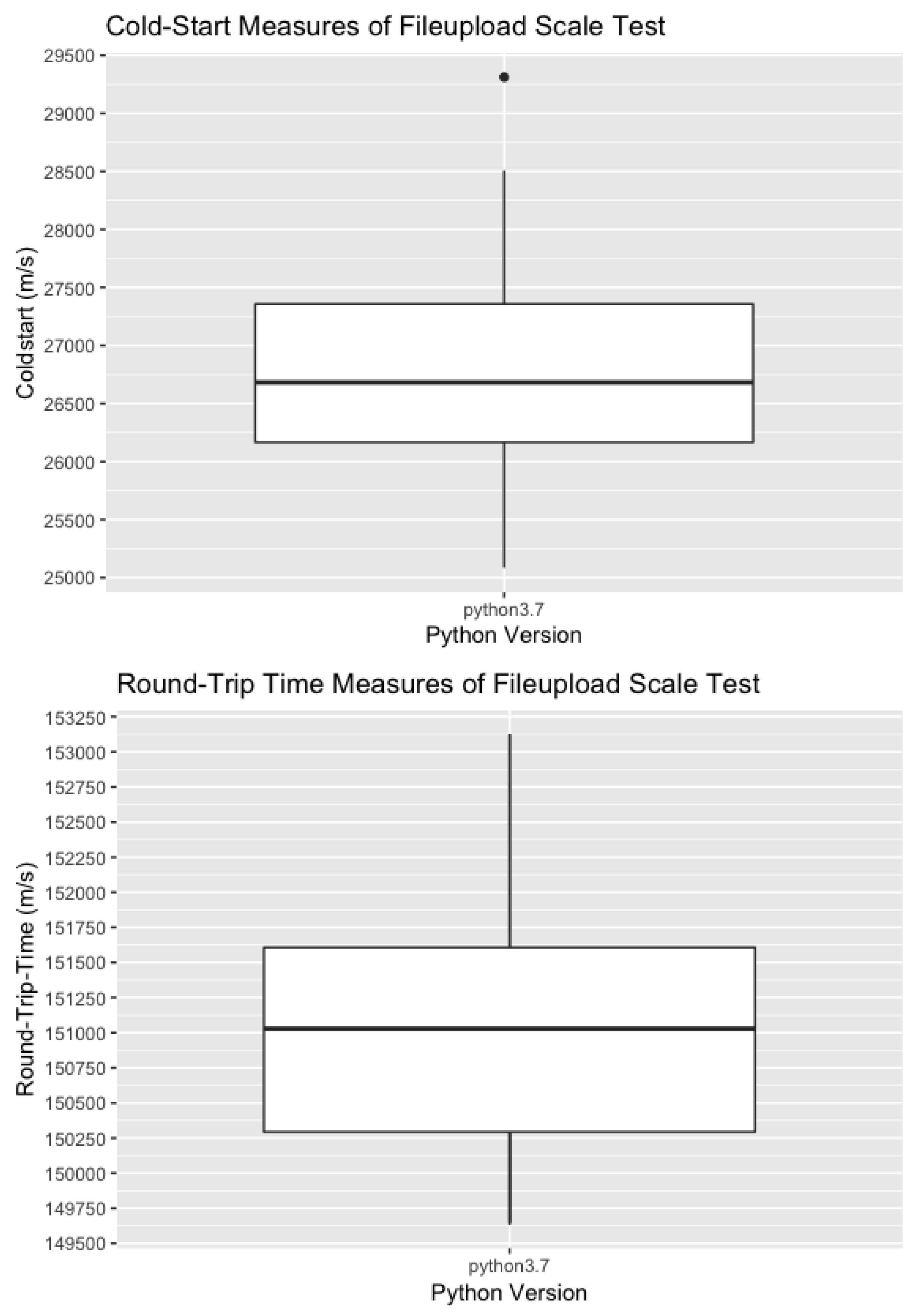
Scale Test: The Scale Test run with the integrated file upload streams results in 112 observations and 112 unique functions, with 56 measurement functions per memory size. Each function instance was invoked between 0 and 10 times. The varying timestamps in the dataset indicate that all concurrent invocations result in concurrently running (and therefore contesting) function instances, as requests were sent to different functions interchangeably. The Cold-Start and Round-Trip-Time Boxplot are depicted in Figure 4.
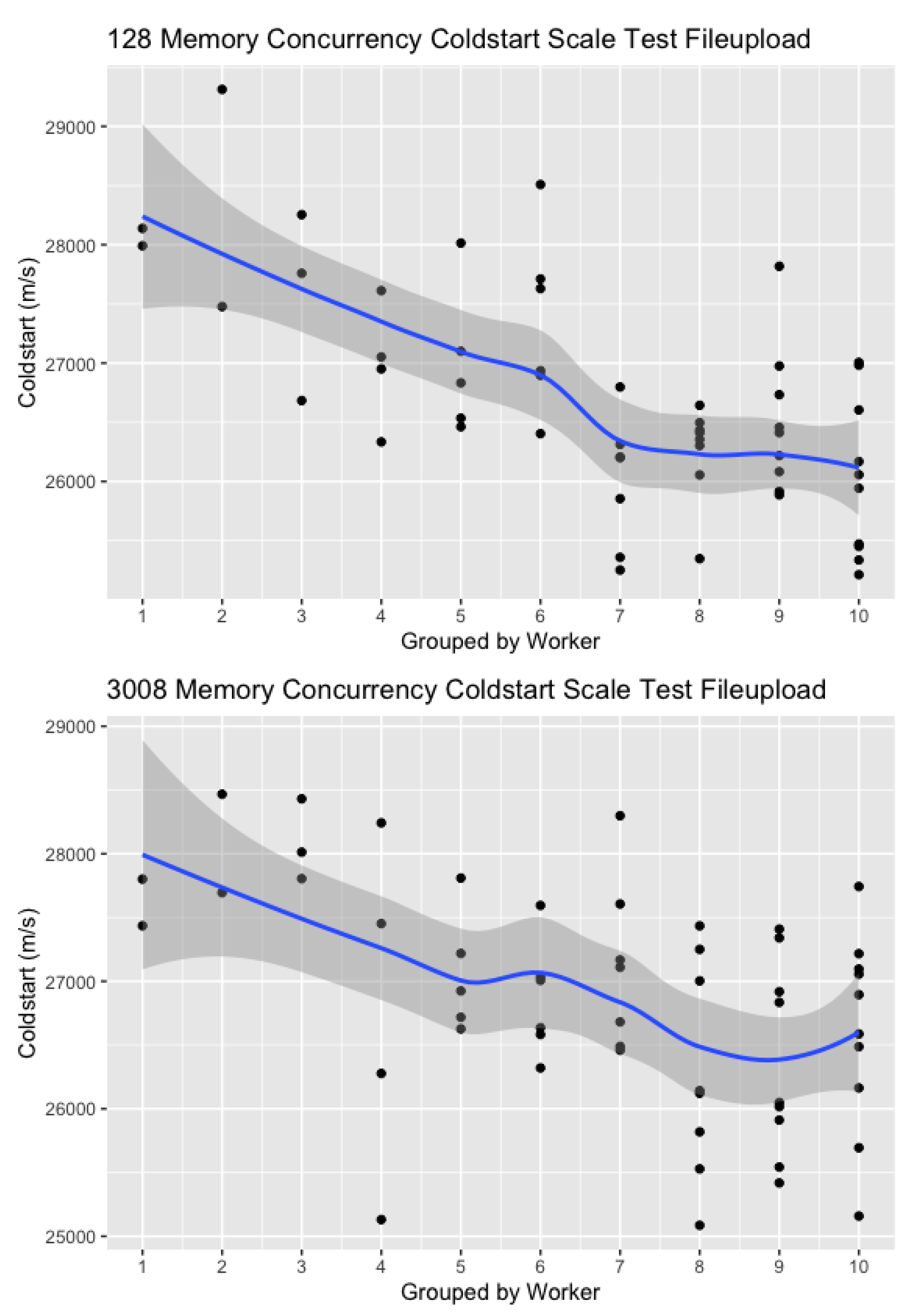
The standard deviation of the Scale Test results is higher than the one identified for the File Upload Cold-Start Test. With the Cold-Start making up 17.66% of Round-Trip Time, scaling up overall leads to higher latency bounds, on average (Table 6). Figure 5 however shows that, with an increasing number of observations, Cold-Start latency tends to decrease. In numbers, this drops from 28,000 to 26,000 ms, thus down 2 s. The steady decrease may be caused by a usage of warm instances, as with each added concurrent request, a new instance is launched but the previous ones are likely taken from the warm queue. However, only two VMs can be identified that are reused, and subsequent requests were sent to those function instances. A second reason for the lower time may be that taken from the theoretical background, where the resource allocation and instance provision quickens after a function has been called for the first time. The decrease in numbers is likely caused by the influence of both, and possibly a close cluster locality.
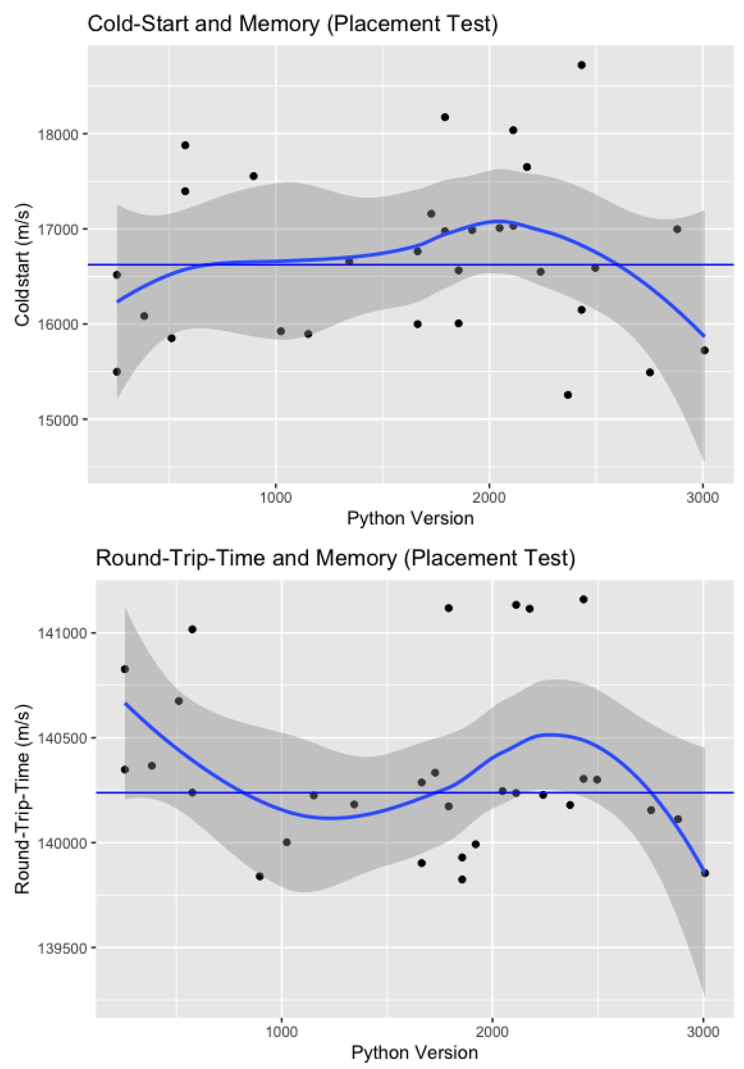
Placement Test: The Placement Test deployed 30 function instances of different memory sizes; however, the data show that seven of them were randomly specified twice. The Cold-Start and Round-Trip-Time Boxplot are visualised in Figure 6.
Round-Trip Time and Cold-Start are both affected by the chosen memory size. The graph shows that the memory size corresponding to the function instance impacts the Cold-Start latency. However, these fluctuations seem to be random as there are high and low values for both small and large memory sizes. To further investigate this, a correlation test has been carried out. With a correlation value of 0.056, no significant correlation between memory and Cold-Start can be detected. In general, the changes may be random because Cold-Start naturally varies, as shown in the previous test results. In addition, each function was only invoked once and the dataset, therefore, does not provide statistical evidence. Despite varying memory sizes, no VM can be identified as duplicated in the dataset, but the vCPU (virtual CPU) number and processor model is the same for all instances.
4.1.2. Findings
To begin with, the data indicate a strong contribution to the time indicators from the environment, as executions were on average over 20 s long. The code of the handler function contains sub-processing and requires libraries that need to be loaded, thus increasing the instance provisioning and execution time. Therefore, the numbers need to be considered carefully and may only indicate trends. Caused by the small size of the dataset, it is not consistent and rather varies, so the standard deviation was used in most cases to indicate statistical evidence of the trends. Hence, all data need to be weighed up further to provide adequate statements regarding the research questions.
Architecture and VM Hardware: Across all experiments including test runs, over 300 functions were deployed. With two exceptions of 3 GHz, all data indicate an Intel(R) Xeon Processor @ 2.50 GHz and 2 vCPU on the underlying VM. The timestamps indicate that the majority of functions were invoked alternately. Thus, the data do not provide significant evidence that with scaling up, the same set of VMs is reused.
Cold-Start Latency and Round-Trip-Time: Python versions newer than 2.7 seem to result in slightly lower Cold-Start times and Round-Trip times. This can be supported by the median of the two measurements being similar to the File Upload Stream Cold-Start Test with Version 3.7, and the overall result of the Python Version Test, where 2/3 of the observations were using newer runtimes. Thus, there is a possibility that AWS better supports newer runtimes. With the integration of the File Upload Stream, the standard deviation increases, as when scaling up. This is likely caused by the necessary call to the external service. An explanation may be that Cold-Start remains stable on average because setting up the instance does not entail the AWS S3 call yet, which forms a part of the Round-Trip time. This requires a further investigation of the influence of the method of triggering the function, and again on a larger dataset.
When comparing the memory sizes, a slight decrease of Cold-Start and Round-Trip time for the higher memory can be identified. In comparison with Figure 6 from the Placement Test, a decreasing trend for memory sizes higher than 2624 MB (64 × 6) can be confirmed. Therefore, the results indicate that with sufficiently high memory size, the Round-Trip time decreases. It is questionable how valid these results are, especially as the Cold-Start varies drastically. As outlined in the literature review, CPU allocation is memory dependent, with the result that with more memory demand, more CPU share is attached, which could then result in a decreasing Round-Trip time. The CPU share however is independent of the Cold-Start, so the time to set up the VM is not correlated with memory, as the statistical test has also shown. In general, free space must be available on VMs to ensure a fast instance launch; therefore, the framework function probably demands a high memory, which may be made available quickly by a capacity margin on the VMs enabling a faster Cold-Start.
Private and Public IPs: The private instance IP resulted in the same IP across all functions (169.254.76.1). The 169.254.X domain range is a public IP to link local addresses and is used for private routing of metadata via HTTP in a cloud environment. It is likely that, in Serverless, it is used to shift the Lambda configuration information from where it is stored to the instance. The private VM IP however is changing with almost every invocation, as well as the public VM IP. AWS was observed to put only one instance of each account on each VM, so that if the instance changes and a new one must be launched, another VM will be used. VMs were only reused for subsequent requests in a few cases, as concluded from duplicated VMs and instance IPs and their corresponding IDs.
Table 7, Table 8 and Table 9 demonstrate a subset of the dataset to show example observations of reused VMs for each of the three different language versions used in the first test run. Overall, VMs were not reused more than twice in the experiments, and other instances were invoked in between subsequent calls. It can be concluded that the VMs remained in an idle wait period. This can be demonstrated by the changing index, for example, Nos. 5 and 8, and the varying results for the Cold-Start. In the case of the first VM (red), the Cold-Start decreases with the first reuse, but for the second instance latency increases (blue) (Table 9). Furthermore, the table provides evidence that unique instances of IDs and IPs correspond to a unique public IP, and, with a changing set, the VM also changes. The request-id changes with every request.
To conclude, the measurement of the functions show that instances do not share VMs. The Cold-Start and Round-Trip times also fluctuate naturally, but slightly more with the integration of an external service such as AWS S3. Cold-Start was up to 17% of the Round-Trip time. Furthermore, AWS was able to achieve lower Round-Trip time with scaling up and sufficient attached memory. On the one hand, the results from the Placement Test support the theory of a bin-packing approach to allocate resources based on available memory utilisation rates. This could result in less or more Cold-Starts depending on available spots. On the other hand, the usage of the same type of VM in all cases and the faster allocation for larger memory cases show that each VM may have a margin applied and thus available space. Further investigation of this and the CPU share however is out of the scope of this paper, and left to further discussion.
4.2. Traffic Distribution Analysis
The second set of experiments focused on the networking aspects of the scaling practices to measure performance directly, based on the request-response rate and the allocation of VMs for a single function instance. Thus, the results from the measurement functions were used to identify private instance IPs and public VM IPs and determine the distribution of the incoming workloads across the backend infrastructure on a large scale. Through the usage of an AWS Gateway address, Lambda was invoked via HTTP calls and the TCP stack, which were tested on performance as well. An increased invocation rate challenges the network requiring tighter latency bounds, as concurrency and contention play an important part in the performance. The data from the 24-h interval run to collect data on AWS Lambda infrastructure traffic and performance is visualised in a distribution of the IP addresses and requests over the interval considered.
Collecting and investigating flow information is important to evaluate the overall quality and performance of the network and can be indicated through certain metrics. Such key performance indicators may be Latency Indicators. The most important indicator is the Round-Trip Time, defining the intervals between a sender transmitting a request segment (SYN) and reception of its corresponding acknowledgment segment (ACK), and the subsequent data transfer time. As this time influences propagation, processing and queuing times in the routing, it must be kept low. Another indicator is the Connection Set-Up Time, which refers to the interval that is necessary to establish a new TCP connection by performing a three-way handshake and is influenced by scheduling. Metrics to distinguish connection time must be measured bi-directorial, and the location of the passive monitoring node on the connection route is important. By subtracting the timestamp values of the two segments, one can calculate the estimation of this value. As the TCP stack also influences data processing, the throughput rate or data transfer time indicating the time to answer a request is another Key Performance Indicator, influenced by the arrival rate, response time and possible Cold-Start [16,17].
For the experimental set-up, a single Lambda Function with the File Upload Stream handler code was deployed on AWS and an API Gateway layer was added with SAM [23]. The API takes a .txt file as an example file type, triggers the function for its encoding, and adds it to the same AWS S3 folder. There is a 200 OK JSON message returned from the handler function, so a successful request can be identified. The function can be triggered by a POST Request. To aid with generating a high request volume, a customised bash script was used to frame the request in suitable interval rounds with randomised initialisation. The script was written to run in a 24-h test run. The settings were randomised to avoid possible pattern recognition by the AWS Load Balancer. Furthermore, the intervals were roughly based on the average distribution of web traffic over a day, with increasing events during daytime and a high frequency of requests in the evening, and a low at night according to the literature examples [24].
4.2.1. Experimental Results
The results from the different test runs are summarised as follows. The requests for the initialisation of the functions were carried out with a random sleep time of 1–10 min depending on the interval. Figure 7 describes the number of invocations over the experiment time.
Figure 7 displays how the script generated changing request rates for each interval. This results in fewer invocations in the morning and at night, with a peak in the afternoon (3:00 pm local time).
Figure 8 shows the concurrent executions over time. The data are generated according to the specifications in the script, with 1–4 concurrent requests depending on the interval.
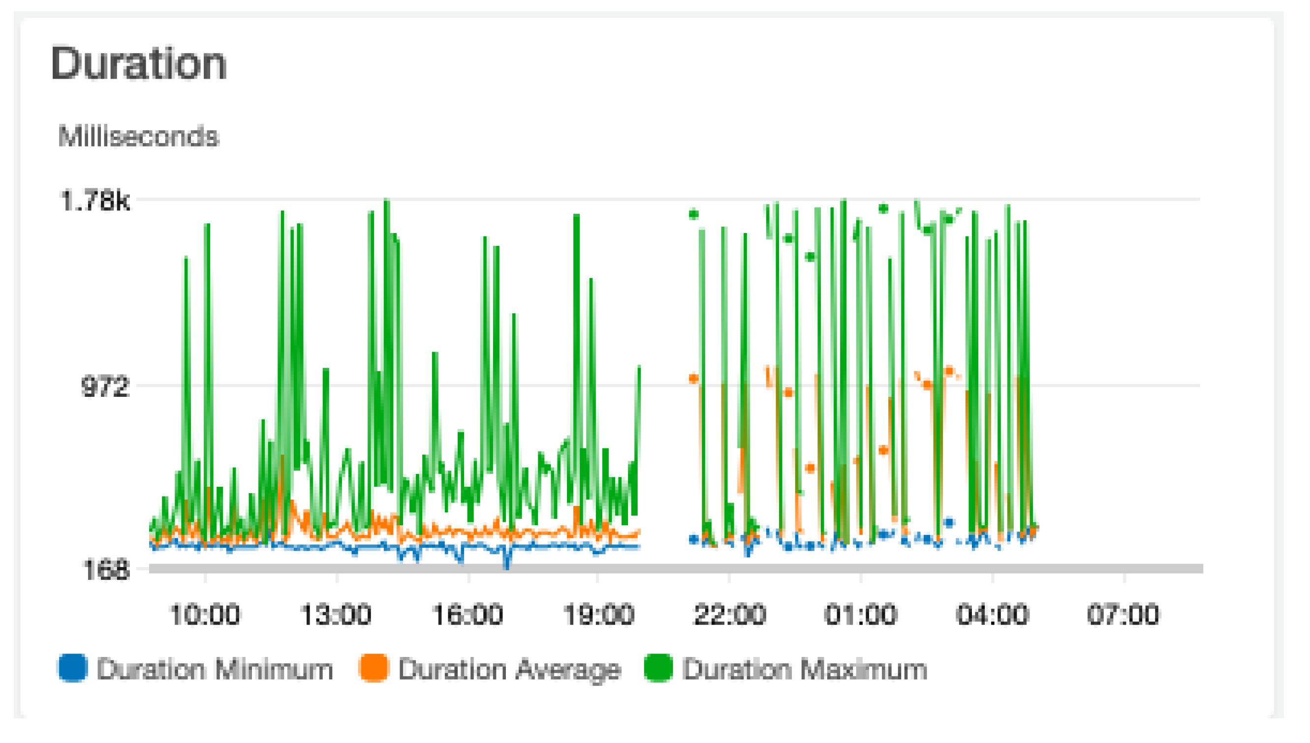
A range of CloudWatch Insight queries was applied to the data to identify patterns regarding performance indicators. The first step in the process of measuring performance is the execution time. An overview of the execution time was conducted from CloudWatch (Figure 9).
The graphs clearly show how execution time and thus performance differs within the intervals as well as between intervals. Especially Interval 6, with a random sleep time of up to 10 min, shows a more frequent higher duration and a higher duration average, indicated by the orange dots after 10 pm, as shown in the graph. However, there is an overall pattern of periodically changing execution time regardless of large numbers of concurrent requests.
The quantile calculation shows that the largest part of requests took 200–800 ms with a mean of 346.83 ms. The initDuarion median across all intervals was identified as 302 ms. The memory usage on average was 78 MB, which is below the specified minimum level of 128 MB.
The varying results demonstrate how traffic in a Serverless environment is influenced by the performance of the underlying system. Execution time therefore depends on both hardware and software configuration, the algorithms applied and the network itself. Hence, the data are open to further discussion.
4.2.2. Findings
Further manipulation of the dataset has been carried out in R Studio to determine results regarding auto-scaling and its impact on load balancing. As concluded from the previous tests, the change of private and public VM IP addresses simultaneously indicates the use of a different instance to handle the request. Thus, the private instance IPs were isolated from the logs and subjected to a time series analysis to determine changes of the VM with the incoming request rate.
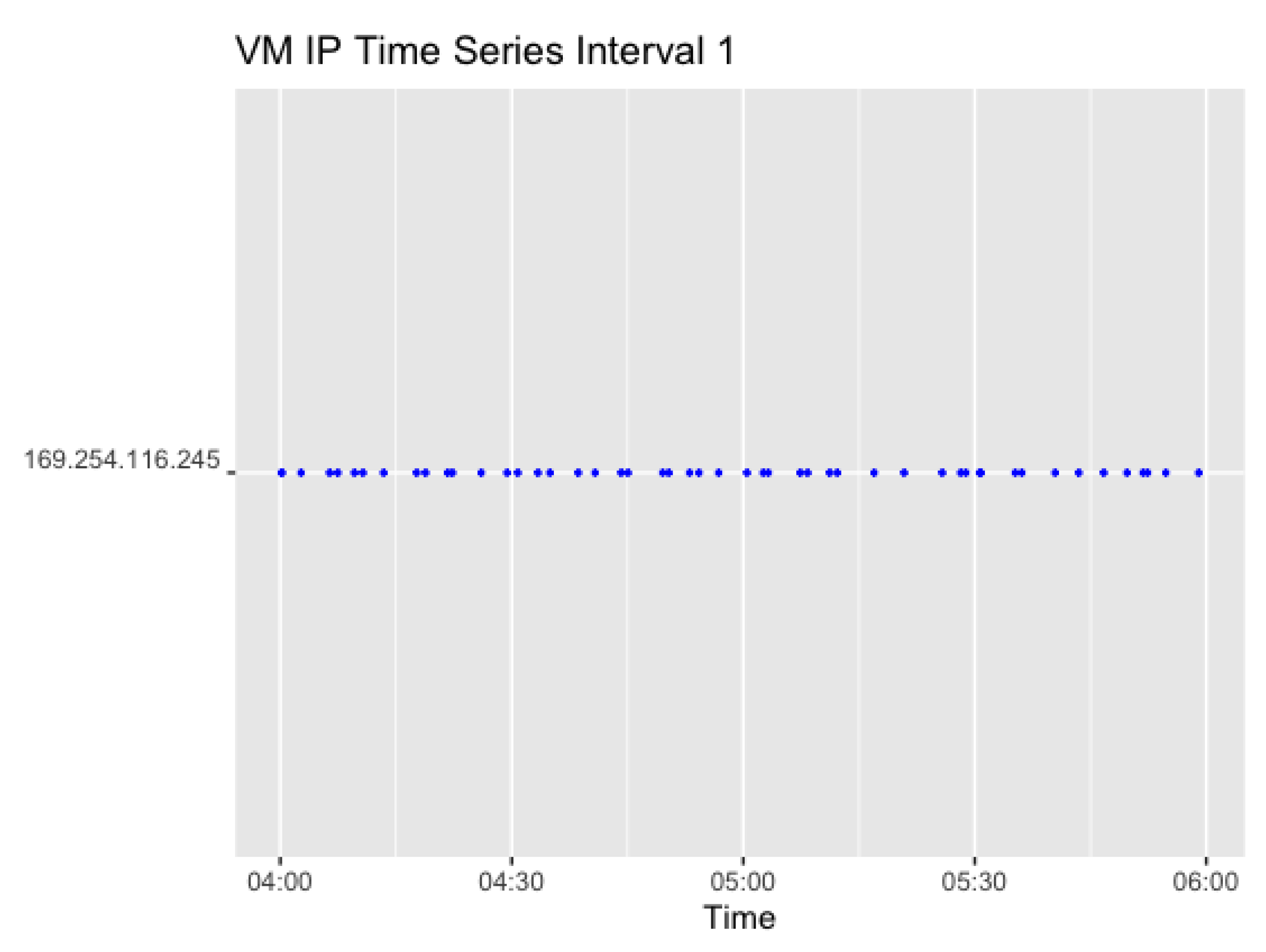
For Interval 1, with a request rate of one invocation every 1–5 min over 5 h, only one IP address was identified for 50 observations. In this case, subsequent requests were sent to the same VM and it can be concluded that the instance remained warm over the entire period. The result is displayed in Figure 10.
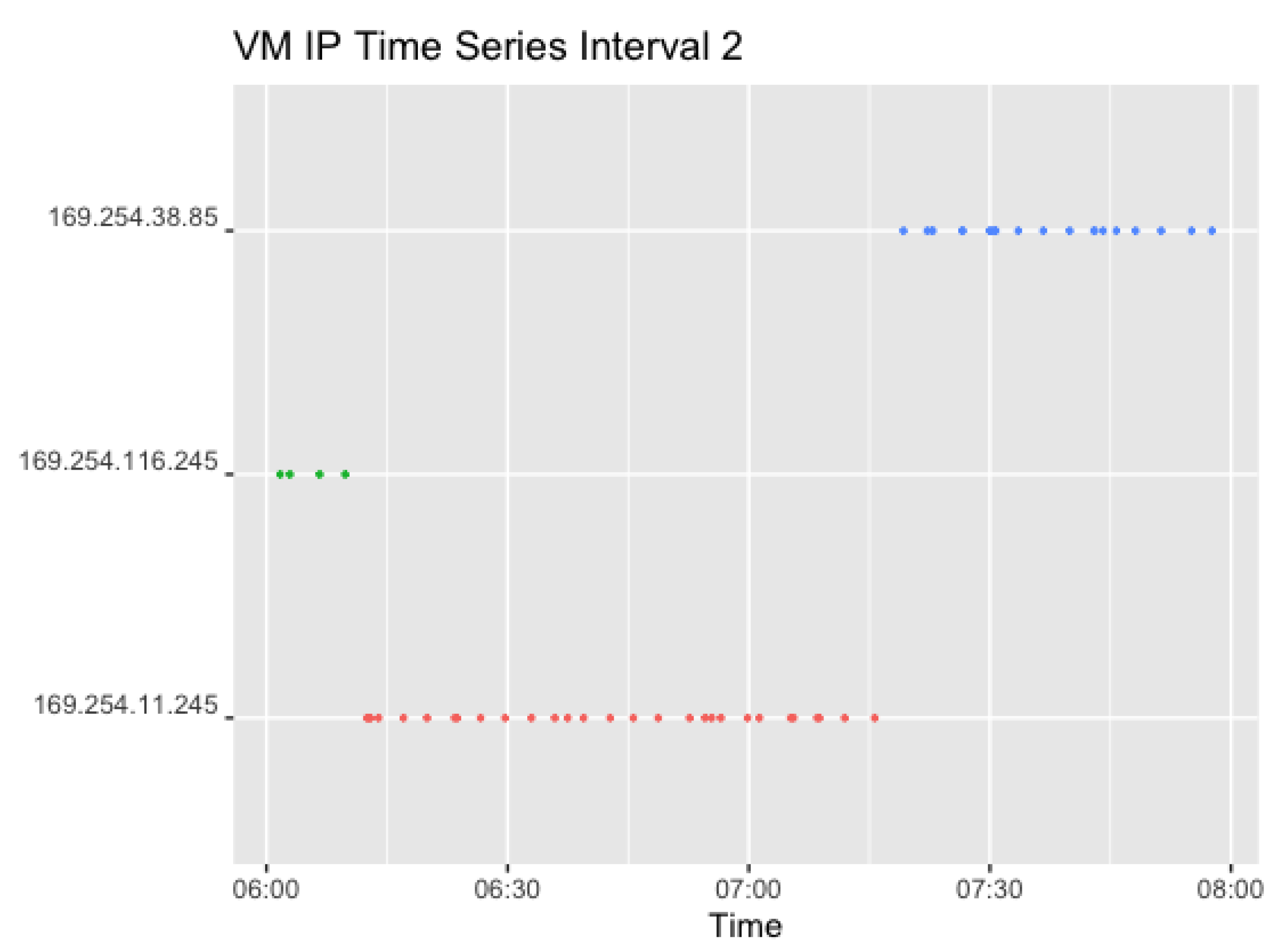
Figure 11 shows the corresponding plots for Interval 2. Interval 2 sends a request in a 0–4 min random interval, which resulted in 54 observations. The difference in color indicates a different VM, which changes twice in the given interval. The first IP (169.254.116.245) was used further following Interval 1.
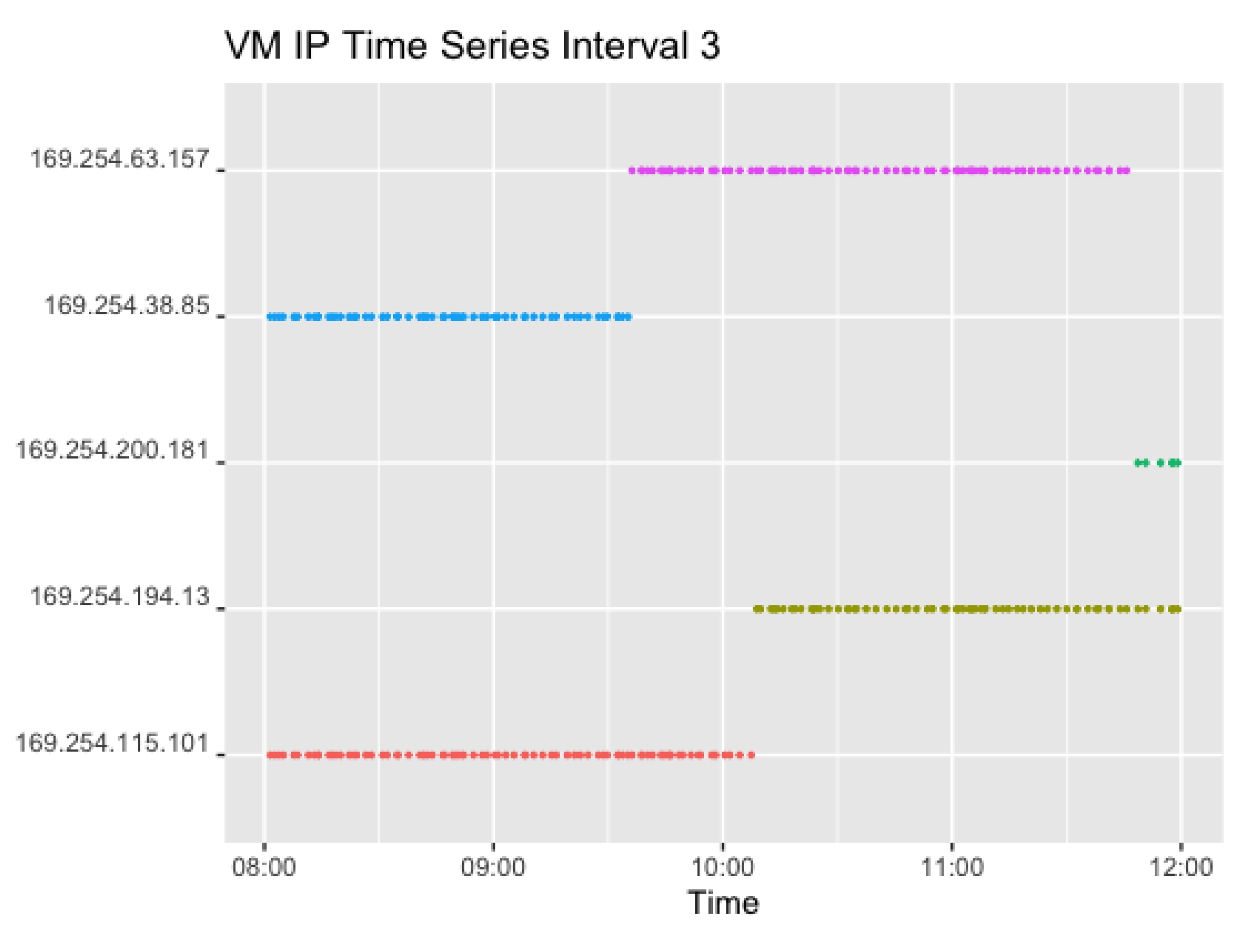
Figure 12 shows the corresponding plots for Interval 3. Interval 3 sends two concurrent requests in an interval of 0–3 min, which resulted in 306 observations. Here, the graph shows two IPs for each timestamp.
This shows that the IPs in Interval 3 changed thrice within the given time frame. However, Interval 3 lasted 2 h longer than Interval 2. In addition to that, only one VM was changed at a time, as can be seen for the first time around 9:30 pm. In addition, the IP at the end of the second interval (169.254.38.85) and thus the VM was used further in the next interval, and changed after a total of around 2 h of usage. The second VM also changed after around 2 h.
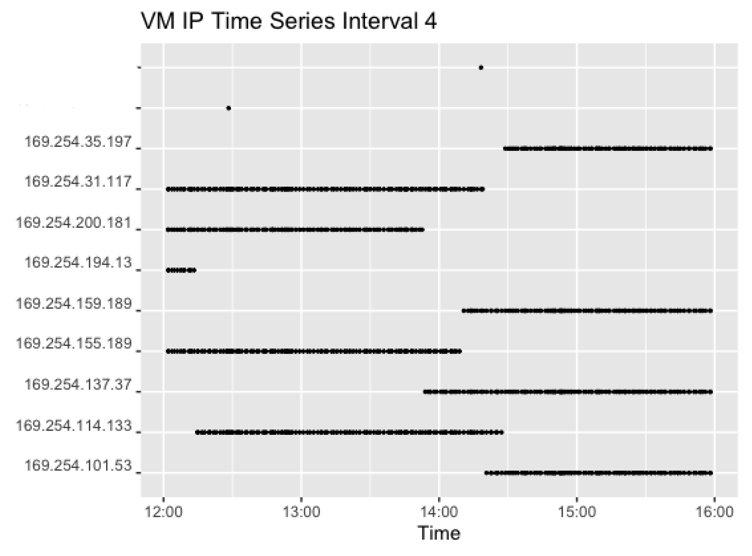
Figure 13 and Figure 14 show the corresponding plots for Interval 4 and 5. Interval 4 sent four concurrent requests in a 0–3-min interval while Interval 5 sent two concurrent requests in an interval of 0–2 min. Hence, Figure 14 shows two IPs for each timestamp. That resulted in 930 observations for Interval 4 and 920 observations for Interval 5.
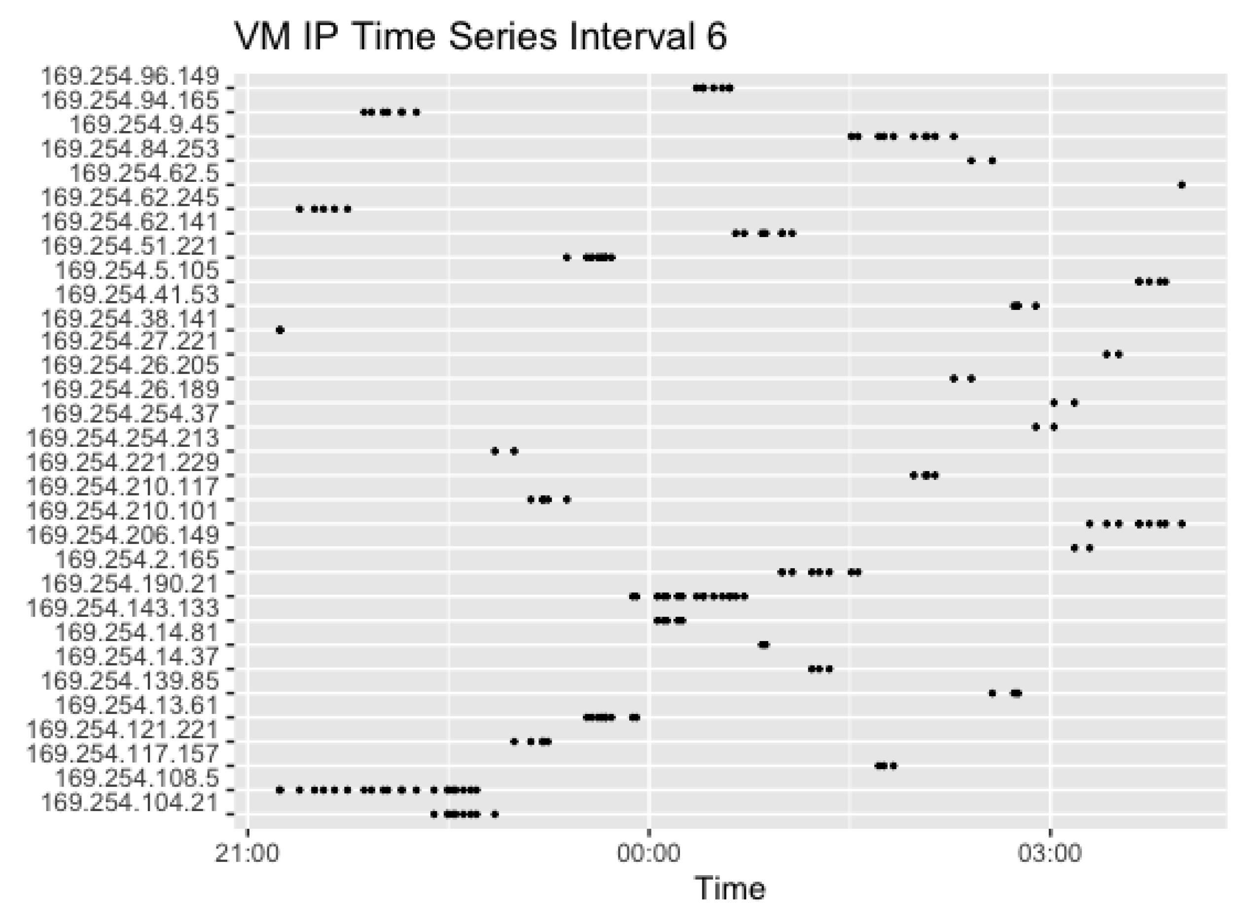
Interval 4 shows the use of the set of IP addresses following the end of Interval 3, but added two extra as the number of concurrent requests rose. Again, the set of VMs changed after around 2 h. In Interval 5, however, all four IPs previously used in Interval 4 stayed warm, but seem to have been reused after pausing. This is most likely caused by the high request rate, where the instances are needed when the previous requests have not yet returned. Lastly, Figure 15 shows the corresponding plot for Interval 6. In the last interval, the request rate of two concurrent requests with a random sleep time of 0–10 min resulted in 174 observations overall.
In this Interval, the IP address was changing more frequently. This is likely to be caused by a low request rate of up to 10 min. With a smaller random generated sleep time, the VM may be idle and available for reuse. However, with a longer wait period, the likelihood of the VM getting cold, requiring the launch of a new VM, increases.
Counting the overall usage of Instance IP Addresses, Table 10 gives an overview of the number of invocations indicated by the number of instances used, and the number of VMs indicated by the public IPs used, for each interval.
There are 51 distinct IP addresses in the dataset. The distribution of the IP addresses shows that, unlike in Measurement Framework results, VMs were reused more than twice, and reused immediately afterwards. During Interval 2 (0–2 min sleep time), Interval 3 (0–3 min sleep time), Interval 4 (0–4 min sleep time) and Interval 5 (0–1 min sleep time), the IP addresses remained stable for a certain period before changing to another set. This happens after around 2 h, regardless of a continuing request rate. In Interval 6, however, the addresses changed with almost every invocation. This indicates that AWS tends to schedule subsequent requests to the same, warm VMs for the most part. However, the more IP addresses change, the longer is the wait time between intervals, which indicates that instances go cold after around 10 min. In between intervals, however, the same VMs used during the last invocations of the previous intervals continued to be used, and more instances are launched in the case of a higher request rate. In addition to that, AWS was observed to not reuse VMs after changing the settings, and seem to not place more than one instance on a VM, thus confirming the results from the measurement test.
A major finding of the time series analysis is that VMs seem to change regardless of the changes in the request-rate. That means, that AWS was observed to allocate subsequent requests to another VM after a certain time automatically, regardless of the incoming request frequency changes. That appears true also for concurrent requests, whereas only one VM IP changes at a time. In the event of allocating the traffic to another resource, the previous instance must go cold and a new instance must be launched on that VM. As a result, this increases the execution time and thus explains the changing duration as displayed in Figure 9. However, the data do not provide enough detail on the exact timing of the changes, which remains subject to further investigation. It can be concluded that each instance has not only an idle-time but also a life-time.
Architecture: In comparison with the previous results from the measurement framework tests, the data from the Traffic Distribution Analysis logs again show the same private instance IP for the Lambda functions. As a link local network, it is possible that the IP is changing regardless within clusters, as it can be allocated within each network domain. This would suggest that AWS allocates the IP not to an instance, but to an account. However, investigation of this requires further discussion.
In terms of the underlying hardware, all 2432 observations were analysed in terms of CPU usage and memory. In line with the findings from the Function Distribution Measurement, requests ended at the same type of server with an Intel(R) Xeon(R) Processor @ 2.50GHz and 2 vCPU for the majority of observations. However, 16 observation were placed on a Intel(R) Xeon(R) Processor @ 3.00GHz. Table 11 overviews the range of the collected data.
According to AWS, CPU is shared in fractions of milliseconds, in which each running instance can use it. The share itself is proportional to memory, meaning that theoretically, a higher memory requirement will receive more CPU power [4]. In the case of the file upload stream, however, the share is attached to the allocated 128 MB memory, of which no more than 77 MB is used as described previously. The cached memory variable provides information that, among all executions, usage averaged between 71 kB and 77 MB.
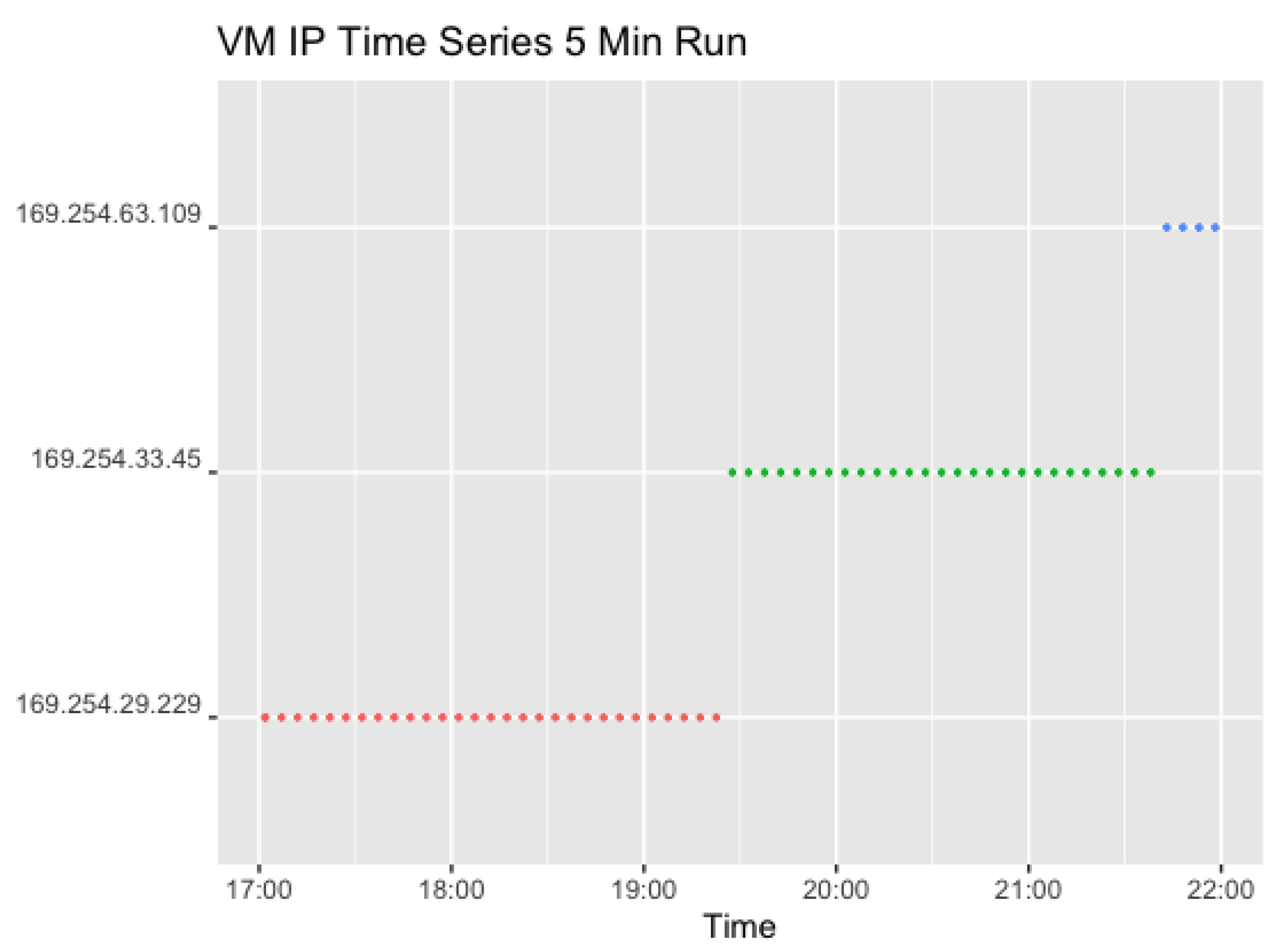
Additional Interval Run: To further explore these findings, a second test run was carried out. The goal was specifically to target the automatic change of VMs. Two sets over 4 h with a request rate of either 5- or 12-min intervals were used to investigate the resource allocation with warm and cold VMs, and the handling of subsequent calls without the influence of randomisation. The test found three distinct IPs for the 5-min run with single requests and 51 distinct IPs for the 12-min intervals with two concurrent requests. There were 61 invocations in the first run and 51 for the second.
As the request settings did not contain any randomised values, the data can be used to validate further the theory resulting from the previous experiment that AWS changes the VM used automatically after a certain period, despite a steady request rate and corresponding warm instances. The results for the 5 min run are illustrated in Figure 16.
Figure 16 again indicates a change in VM after a little over 2 h, which occurs twice in the dataset. The initDuration variable logged by AWS Lambda appeared two times accordingly. As public and private IPs change at the same time, this further validates the conclusion from previous experiments that each private VM IP is attached to a single public IP which does not just change by random IP allocation.
The first change in IP addresses can be observed after the first 30 invocations, and the second after the following 27 invocations. The experiment started at 27 July 2020 17:01:43 (local time). It was ensured that there were no previous invocations for 30 min before starting the experiment. At 27 July 2020 19:27:32 (local time), the first change of IP addresses can be identified. Subtracting these times results in a period of 2 h 24 min 49 s. For the second change, the calculation shows that the VM was running for 2 h 15 min 31 s before changing.
Table 12 overviews the “REPORT” variables of the previous request and the request where the VM first changes.
In the example above, the total execution duration for a new VM event changed around 364.23%, which thereby increased the billed duration as well. The initDuration made up 17.21% of the total duration, which is similar to the percentage taken from the measurement framework tests. Moving on to the subsequent request, the execution duration decreased again to a normal level (374.34 ms).
In line with the findings of Interval 6, this shows 51 distinct IP addresses, resulting in a new pair at each invocation. The larger wait time between workloads, therefore, leads to the instances going cold. A new instance is initialised every time.
“Hello World” Run: A separate function instance only returning a simple Hello World message was used to be compared to the File Upload Stream. The average execution time of the Hello World Function according to Cloud Watch Insights lay between 15 and 79 ms with a mean duration of 36.6 ms. Compared with the File Upload Stream execution mean of 346.83 ms, the execution time increased by around 840% with the integration of the API Gateway, S3 and the calculations of the underlying procs files.
To further investigate the automatic changing of VMs, the request rate was set for 1 and 10 min for this test run, resulting in 288 observations overall. The results again validate the previous findings of the automatic change in VMs after around 2 h. However, there is not a change with every request for the 10-min interval. A separate test with an 11-min interval again showed no change, but it did with a 12-min interval. Therefore, it can be concluded that an instance has an idle time of around 12 min. Figure 17 overviews the results.
The Hello World function was also deployed in a different region, eu-west-2, to investigate possible changes in traffic. The IP addresses identified were within the AWS IP range of 3.x, 18.x, 32.x, 35.x, 52.x and 54.x. across all IPs collected in the study, but with a different location in London, UK. However, the private instance IP remains the same as in the us-west-1 region (169.254.76.1).
Postman Results: With the use of the REST API Gateway for Lambda, an HTTP POST call can be made over TCP, where a three-way-handshake is made before the request is sent out through the webserver. In this way, it is possible to trigger the function directly from the client’s browser, including a data transfer. Carrying out a sub-experiment with Postman [18] to further break down the network protocol stack for the TCP packets for the File Upload Stream, we can determine the time taken to fulfill the three-way-handshake (SYN-ACK time) and Round-Trip time for different request timings, to identify the impact of the gateway on load balancing and latency. In addition, these results may serve to determine the effect of Cold-Start and the client socket on network latency.
Table 13 summarises the results for the Round-Trip time for the wait periods of 20, 15, 12, 10, 5 and 1 min, as well as 1 s.
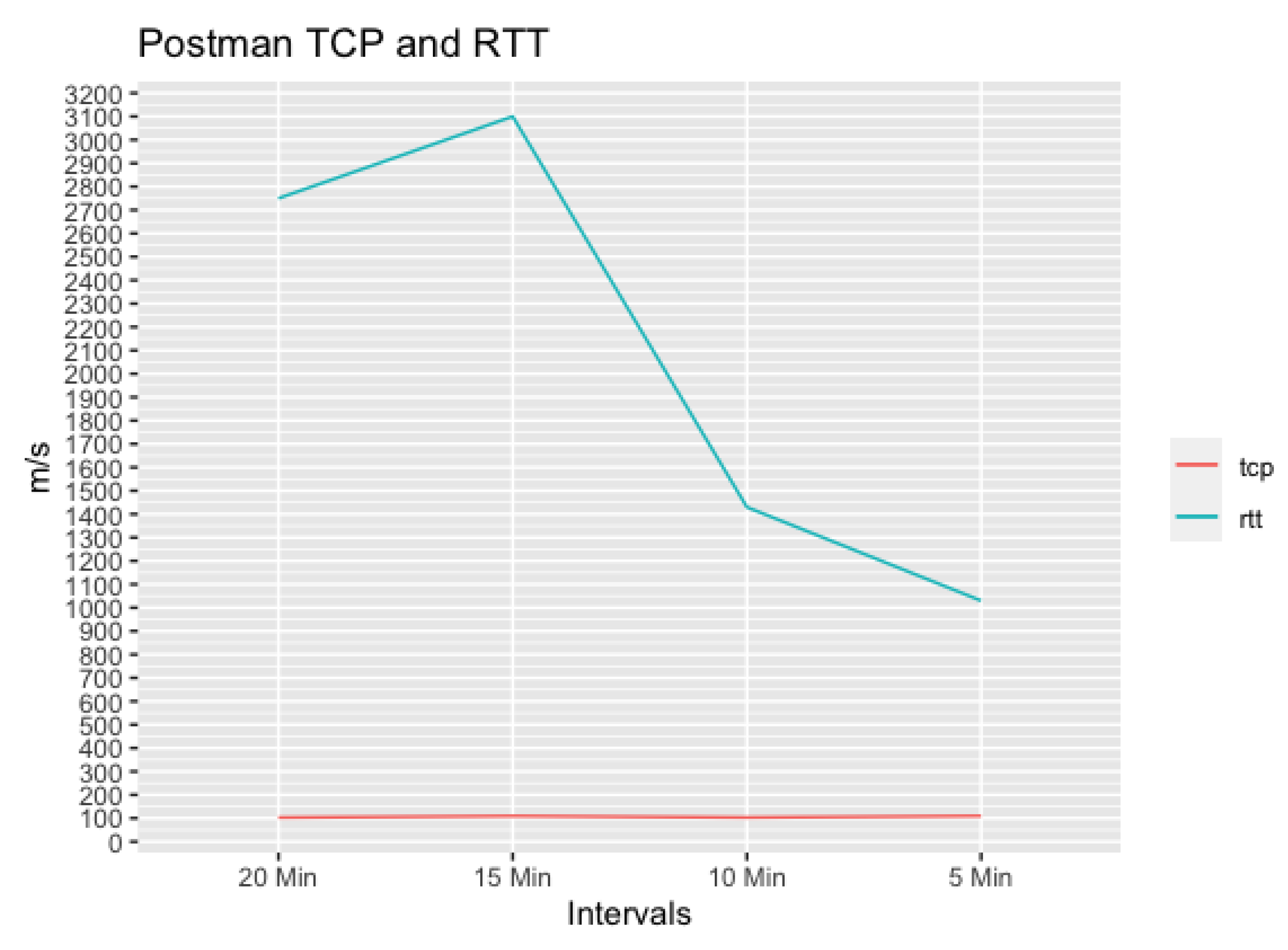
The lowering Round-Trip-time over more frequent requests indicates usage of a warm instance. However, the decreasing rate flattens slightly over a request rate of 1–10 min. For the 15-min intervals, a peak can be observed, which is likely caused by normal fluctuations. In general, the most drastic change can be observed between 12 and 10 min of sleep time, where the Round-Trip-time decreases over 1 ms. The idle period must, therefore, lie in that range, which matches the previous findings.
Compared to the Execution Time on AWS Lambda for the Traffic Distribution Analysis averaging around 346 ms, the Postman Test shows results between 323.11 and 2110.79 ms with an average of 1027.36 ms. The time difference between the execution duration and Round-Trip time must be caused by provisioning the VM, the connection time and data exchange. This accounts for 1–1.5 s, which appears also in line with the previous results.
For the initial cold run, the time required to fulfill the request for each process is shown in Figure 18.
The Postman results show that the transfer time makes up the most of the request time. It varies depending on the interval, while the TCP Handshake time remains stable. It is likely that the socket initialisation, DNS, TCP and SSL transports are managed by a separate proxy as such calculations are expensive and AWS would benefit from shifting them to a faster hardware. Comparing the TCP and Data Transfer Time, Figure 19 provides an overview and confirms the steady TCP stack implementation time.
To sum up, the Postman Tests provide evidence that the increased latency with long idle times is due to a longer Data Transfer Time, presumably caused by the Cold-Start. The network TCP stack implementation however remains stable, so that the reason for the longer Data Transfer Time must be a delay in the data availability, implicating cache availability at the server. That again is most likely influenced by the connection to AWS S3. As the applied API Gateway is a REST service, its stateless nature and session affinity enables a wait time for the request processing. However, this leads to a decrease in performance.
4.3. Comparison to Related Work
As most of the related academic work has been on measuring performance, traffic influences such as execution duration under various settings are thoroughly studied here. Most of the studies have been conducted in Python, but none with the most recent version 3.7. Wang et al. [9] chose 2.7 and Pelle et al. [21] chose 3.6, for example. The set-up of the Function Measurement experiment was according to settings as described in previous studies, most importantly ensuring that invocation does not suffer throttling or batching of over one test run. These similarities help validate the following comparison of results. Most other experiments however were conducted with 512 MB as an average size of Lambda instances, instead of 128 and 3008 MB as in this study [7].
The overall number of deployed functions sums up to around 300 here, versus Wang et al. [9] who far exceeded this with over 5000. Interestingly, among all these functions, they discovered five CPU configurations of 2.9, 2.8, 2.4 and 2.3 GHz, not including the 2.5 GHz model found in this study. Lloyd et al. [19] however discovered a machine with 2 vCPUs and 3.75 GB physical RAM. AWS must therefore change, or update, their hardware configuration constantly. Pelle et al. [21] found that processor types changed when increasing the memory size, which cannot be confirmed here. They also claimed that below 512 MB memory, one core is used for one individual thread, and more memory simply results in more threads under one core. The data at hand do not indicate that this is the case, and, in comparison to other work, it is unlikely that function instances use the entire core capability. That is probably the case because as discussed previously, the code could not use the extra time. However, the underlying processor is, as discovered by Pelle [21], an Intel Xeon Type. However, the type does not change as they suspected, regardless of the chosen memory size. It is important to mention that AWS changed the Linux version from 2017, which the experiments in their study were carried out on, to a version of 2020, which was used in this experiment. The influence of Linux versions on performance and traffic allocation is out of the scope of this paper and subject to further discussion.
Wang [9] argued that changing VM configurations cause more variation in performance, which might be a reason AWS changed the underlying configuration and set-up of VMs. However, the presence of the Kernel uptime in the dataset confirms the hypothesis that VMs were launched before the instance appears. This again indicates a pool of ready VMs [7,9].
The authors of [7,9] also found that performance is influenced by contention. At the most, our experimentation deployed 200 concurrently running functions, whereas other studies [21] calculated using the old concurrency level of 1000 from 2017. AWS was likely scaled down drastically due to the higher demand for Serverless, or low necessity to supply that many instances at once. The impact of Cold-Start time on latency was determined to be around 1–2 s by Hendrickson et al. [18], which matches the findings from the Cold-Start and Postman Test of around 1–1.5 seconds. However, Hendrickson [18] did not specify his methodology or experimentation in detail, and likely did not integrate an external service such as AWS S3.
Another hypothesis is that the algorithm works with a bin-packing approach, using the memory on existing VMs. In particular, the data from the second experiment does not indicate that VMs are allocated more than one time for memory maximisation, which would also not be in line with academic recommendations for implementing available workload margins.
Furthermore, the results of the experimentation do not confirm a linear decrease in Round-Trip time with more allocated memory as indicated by Wang et al. [9]. That more indicates that CPU usage is Cold-Start independent. This could be caused by instances with higher memory getting more CPU cycles, but the CPU is shared fairly. As the results do not indicate any resource competition, it might be that AWS resolved that issue in a way that evened out the sizes of VMs. Lloyd [19] argued that high memory slows down the code execution and increases latency, as more containers need to be launched.
According to Wang’s [9] findings, the framework would invoke each function twice, thus forcing a cold and warm start. However, the results from our experiment show a difference where, in some observations, subsequent calls on the same machine resulted in higher Cold-Start time. It might be that AWS changed the time interval to be exceeded before an instance becomes idle. During their experiments, they found this time to be around 27 min; however, the results from this experiment and those of Lloyd et al. [19] and McGrath and Brenner [7] provide evidence that the time must rather be within 10–15 min. The traffic analysis has shown that Cold-Start does affect the average execution time tremendously, as demonstrated in the difference between Interval 3 and 6. The median instance lifetime detected by Wang et al. [9] was 6.2 h, with a maximum of 8.3 h. Our traffic analysis experimentation however has indicated a much shorter lifetime, of mostly around 2 h. Wang [9] also argued that placing two different instances on the VM implies resource allocation and thus longer Cold-Start and execution time. However, in the experiment, subsequent calls to the same VM also indicated the same instance, as both have been identified as unique.
Wang’s [9] finding that a function executes in a dedicated function instance can be confirmed, and our observations also match his findings that function instances are reused. Function instances sharing the same instance root ID have the same VM public IP and VM private IP, which again was confirmed in this study.
5. Conclusions and Future Work
The aims of the study arose from the recent call in academia for further investigation into the developing field of Serverless technologies. The performance of function instances is determined by their execution time and the overall latency in the Round-Trip-time. Latency itself is influenced by Cold-Starts, meaning the duration of the auto-scaling process in the event of increasing traffic. During experimentation, two attempts were carried out to analyse the influence of these factors on the example of a basic use-case file upload stream API. The Function Distribution Measurement, which deployed and invoked multiple versions of the service on several machines, all acting on the given AWS S3 resource, calculated the Cold-Start time to make up to 15–17% of the Round-Trip-time, with less influence observed when scaling up the request rates. That accounts for the reuse of instances. Furthermore, the integration of the AWS S3 database contributed the most to latency, meaning latency and Cold-Start are heavily influenced by other cloud services.
It is obvious that, with a growing and trending field such as Serverless, all of the studies’ results are subject to change with any update by the provider. However, the goal of our work is to provide a current snapshot of AWS’s practices regarding traffic allocation and to update previous findings in research. A Serverless environment facilitates system administration operations for basic services, as it suits the event-driven, reactive programming of today with faster development and automated code execution. However, it is not suitable for latency-sensitive applications yet. It is recommended for developers to carefully profile their service demands to better cater for uncertainty and to be sure to adhere to best practices. Furthermore, developers need to make sure the service is fault-tolerant and monitor influences such as memory consumption and execution time. On the provider’s side, it is recommended to further provide runtime support and make information such as Cold-Start practices available to the developers to support their goals and thus attract more customers.
Although this work addresses only periodic traffic patterns, the same principle may be extended to live applications. With the limitation that traffic influences change daily, as does the provider’s handling of it, the request-response-rate is stable in cases where the concurrency level does not exceed 200 requests. Moreover, although it is only a snapshot of the current practice, the work can be generalised to the cases where the instance lifetime and idle time are adequately described in most cases today. It is important to mention also the need to carry out the same investigation for any other provider, as this study focused on AWS only. The analysis can also be generalised to the case where the integration of an external service strongly influences Serverless latency, but the exact amount will need to be tested against each of the possible services. As outlined in the discussion, future research would benefit from more support and transparency on the provider’s platform, to help develop better and more latency-sensitive auto-scaling algorithms, methods for synthesising the connection layers and function reuse, as well as accurate tools for developers.
Author Contributions
All authors contributed in the conceptualisation and methodology of the manuscript; L.M. performed the data preparation, advised by P.J.B.; L.M., C.C. and N.P. contributed in writing; and P.J.B. reviewed and edited the manuscript. All authors have read and agreed to the published version of the manuscript.
Funding
The research leading to these results has been partially supported by the European Commission under the Horizon 2020 Programme, through funding of the CPSOSAWARE project (G.A. No. 871738).
Conflicts of Interest
The authors declare no conflict of interest.
References
- Pitropakis, N.; Darra, E.; Vrakas, N.; Lambrinoudakis, C. It’s All in the Cloud: Reviewing Cloud Security. In Proceedings of the 2013 IEEE 10th International Conference on Autonomic and Trusted Computin, Vietri sul Mare, Italy, 18–21 December 2013; pp. 355–362. [Google Scholar]
- Baldini, I.; Castro, P.; Chang, K.; Cheng, P.; Fink, S.; Ishakian, V.; Mitchell, N.; Muthusamy, V.; Rabbah, R.; Slominski, A.; et al. Serverless computing: Current trends and open problems. In Research Advances in Cloud Computing; Springer: Berlin/Heidelberg, Germany, 2017; pp. 1–20. [Google Scholar]
- Hellerstein, J.M.; Faleiro, J.; Gonzalez, J.E.; Schleier-Smith, J.; Sreekanti, V.; Tumanov, A.; Wu, C. Serverless computing: One step forward, two steps back. arXiv 2018, arXiv:1812.03651. [Google Scholar]
- AWS. Serverless Architectures with AWS Lambda Overview and Best Practices. In Amazon Web Services; AWS: Seattle, WA, USA, 2017. [Google Scholar]
- Malawski, M.; Gajek, A.; Zima, A.; Balis, B.; Figiela, K. Serverless execution of scientific workflows: Experiments with hyperflow, aws lambda and google cloud functions. Future Gener. Comput. Syst. 2017. [Google Scholar] [CrossRef]
- Lowery, C. Emerging Technology Analysis: Serverless Computing and Function Platform as a Service; Gartner Research: Stamford, CT, USA, 2016. [Google Scholar]
- McGrath, G.; Brenner, P.R. Serverless computing: Design, implementation, and performance. In Proceedings of the 2017 IEEE 37th International Conference on Distributed Computing Systems Workshops (ICDCSW), Atlanta, GA, USA, 5–8 June 2017; pp. 405–410. [Google Scholar]
- Leitner, P.; Wittern, E.; Spillner, J.; Hummer, W. A mixed-method empirical study of Function-as-a-Service software development in industrial practice. J. Syst. Softw. 2019, 149, 340–359. [Google Scholar] [CrossRef] [Green Version]
- Wang, L.; Li, M.; Zhang, Y.; Ristenpart, T.; Swift, M. Peeking behind the curtains of serverless platforms. In Proceedings of the 2018 USENIX Annual Technical Conference, USENIX ATC 2018, Boston, MA, USA, 11–13 July 2020; pp. 133–145. [Google Scholar]
- Rajan, R.A.P. A review on serverless architectures-Function as a service (FaaS) in cloud computing. Telkomnika Telecommun. Comput. Electron. Control. 2020, 18, 530–537. [Google Scholar] [CrossRef]
- Hassan, S.; Bahsoon, R. Microservices and their design trade-offs: A self-adaptive roadmap. In Proceedings of the 2016 IEEE International Conference on Services Computing, SCC 2016, San Francisco, CA, USA, 27 June–2 July 2016; pp. 813–818. [Google Scholar] [CrossRef] [Green Version]
- Fox, G.C.; Ishakian, V.; Muthusamy, V.; Slominski, A. First International Workshop on Serverless: Report from workshop and panelon the Status of Serverless Computing and Function-as-a-Service. In Proceedings of the First International Workshop on Serverless Computing (WoSC) 2017, Atlanta, GA, USA, 5 June 2017; pp. 1–22. [Google Scholar]
- Brenner, S.; Kapitza, R. Trust more, serverless. In Proceedings of the 12th ACM International Conference on Systems and Storage, New York, NY, USA, 3–5 June 2019; pp. 33–43. [Google Scholar]
- Yan, M.; Castro, P.; Cheng, P.; Ishakian, V. Building a Chatbot with Serverless Computing. In Proceedings of the 1st International Workshop on Mashups of Things and APIs, Trento, Italy, 12–16 December 2016; pp. 1–4. [Google Scholar]
- Nguyen, H.D.; Zhang, C.; Xiao, Z.; Chien, A.A. Real-time Serverless: Enabling application performance guarantees. In Proceedings of the 5th International Workshop on Serverless Computing, Davis, CA, USA, 9–13 December 2019; pp. 1–6. [Google Scholar] [CrossRef]
- Brozoza, P. Key Performance Indicators of TCP Flows. Tech. Univ. Munich 2018, 1, 105–112. [Google Scholar] [CrossRef]
- Khazaei, H.; Barna, C.; Beigi-Mohammadi, N.; Litoiu, M. Efficiency analysis of provisioning microservices. In Proceedings of the International Conference on Cloud Computing Technology and Science, CloudCom, Luxembourg, 12–15 December 2016; pp. 261–268. [Google Scholar] [CrossRef]
- Hendrickson, S.; Sturdevant, S.; Harter, T. Serverless Computation with OpenLambda. In Proceedings of the USENIX Workshop on Hot Topics in Cloud Computing, Denver, CO, USA, 20–21 June 2016. [Google Scholar]
- Lloyd, W.; Ramesh, S.; Chinthalapati, S.; Ly, L.; Pallickara, S. Serverless Computing: An Investigation of Factors Influencing Microservice Performance. In Proceedings of the 2018 IEEE International Conference on Cloud Engineering (IC2E), Orlando, FL, USA, 17–20 April 2018; pp. 159–169. [Google Scholar]
- Pérez, A.; Moltó, G.; Caballer, M.; Calatrava, A. Serverless computing for container-based architectures. Future Gener. Comput. Syst. 2018, 83, 50–59. [Google Scholar] [CrossRef]
- Pelle, I.; Czentye, J.; Dóka, J.; Sonkoly, B. Towards latency sensitive cloud native applications: A performance study on aws. In Proceedings of the 2019 IEEE 12th International Conference on Cloud Computing (CLOUD), Milan, Italy, 8–13 July 2019; pp. 272–280. [Google Scholar]
- AWS Compute Blog. New for AWS Lambda—Predictable Start-Up Times with Provisioned Concurrency. 2020. Available online: https://aws.amazon.com/blogs/compute/new-for-aws-lambda-predictable-start-up-times-with-provisioned-concurrency/ (accessed on 22 June 2020).
- AWS. AWS Serverless Application Model-Tutorial: Deploying a Hello World Application. 2020. Available online: https://docs.aws.amazon.com/serverless-application-model/latest/developerguide/serverless-getting-started-hello-world.html (accessed on 22 June 2020).
- Morley, J.; Widdicks, K.; Hazas, M. Digitalisation, energy and data demand: The impact of Internet traffic on overall and peak electricity consumption. Energy Res. Soc. Sci. 2018, 38, 128–137. [Google Scholar] [CrossRef]
Figure 1.
Overview of the typical AWS Lambda request procedure.

Figure 2.
Boxplot of Cold-Start and Round-Trip-Time results for different Python versions.
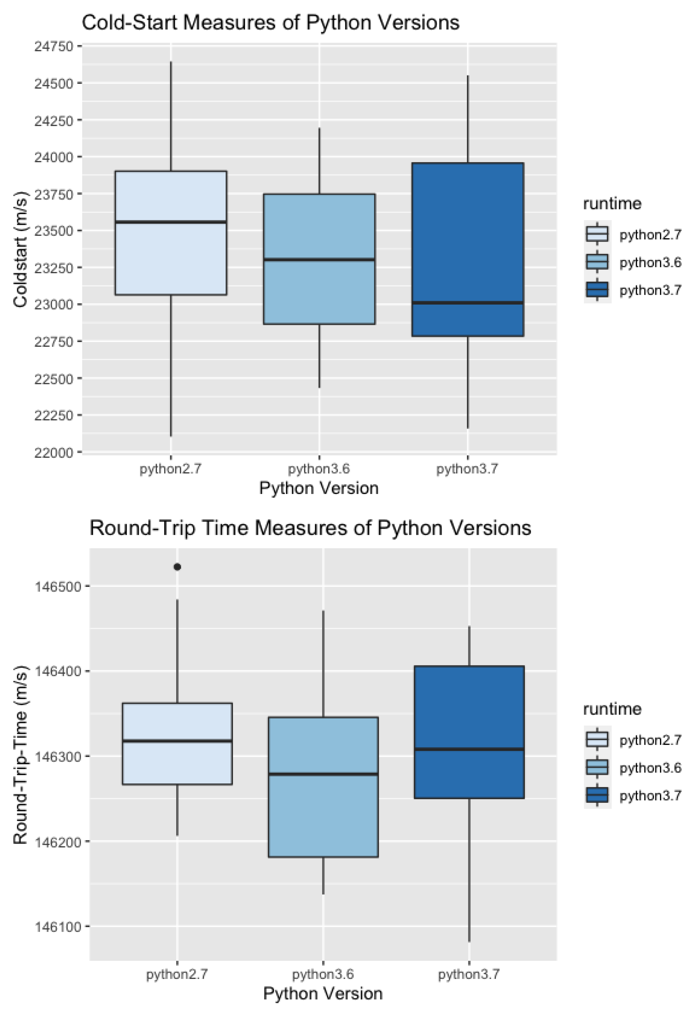
Figure 3.
Boxplot of Cold-Start and Round-Trip-Time Results for integrated Fileupload Stream.
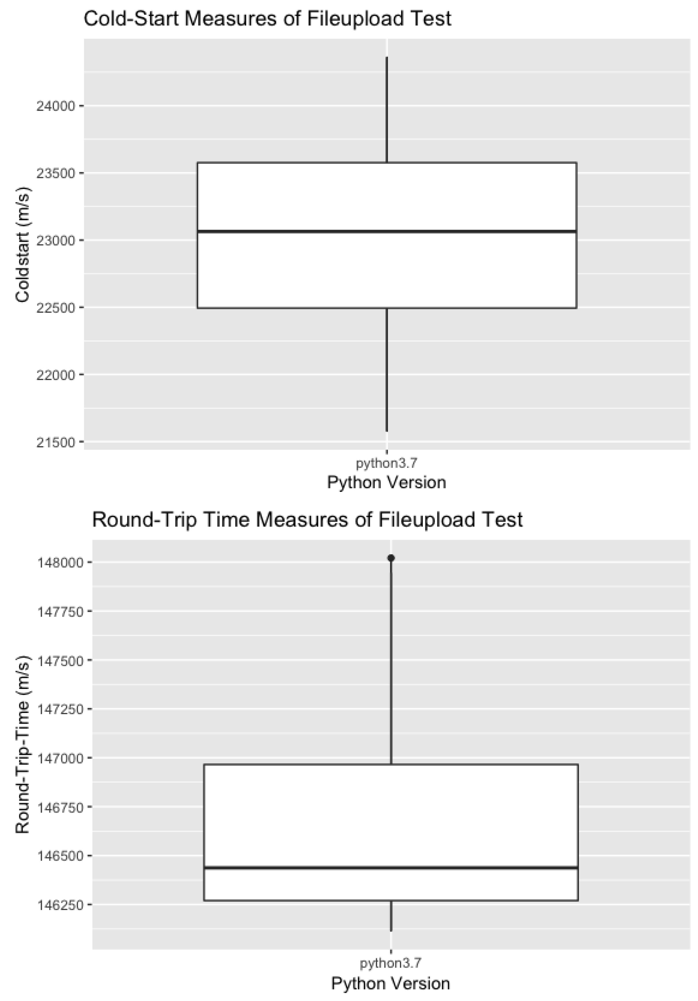
Figure 4.
Boxplot of Scale Test Cold-Start and Round-Trip-Time results for Scale Test.

Figure 5.
Scale Test results Cold-Start Memory.

Figure 6.
Boxplot of Cold-Start and Round-Trip-Time results for Placement Test.

Figure 7.
Intervals invocations.
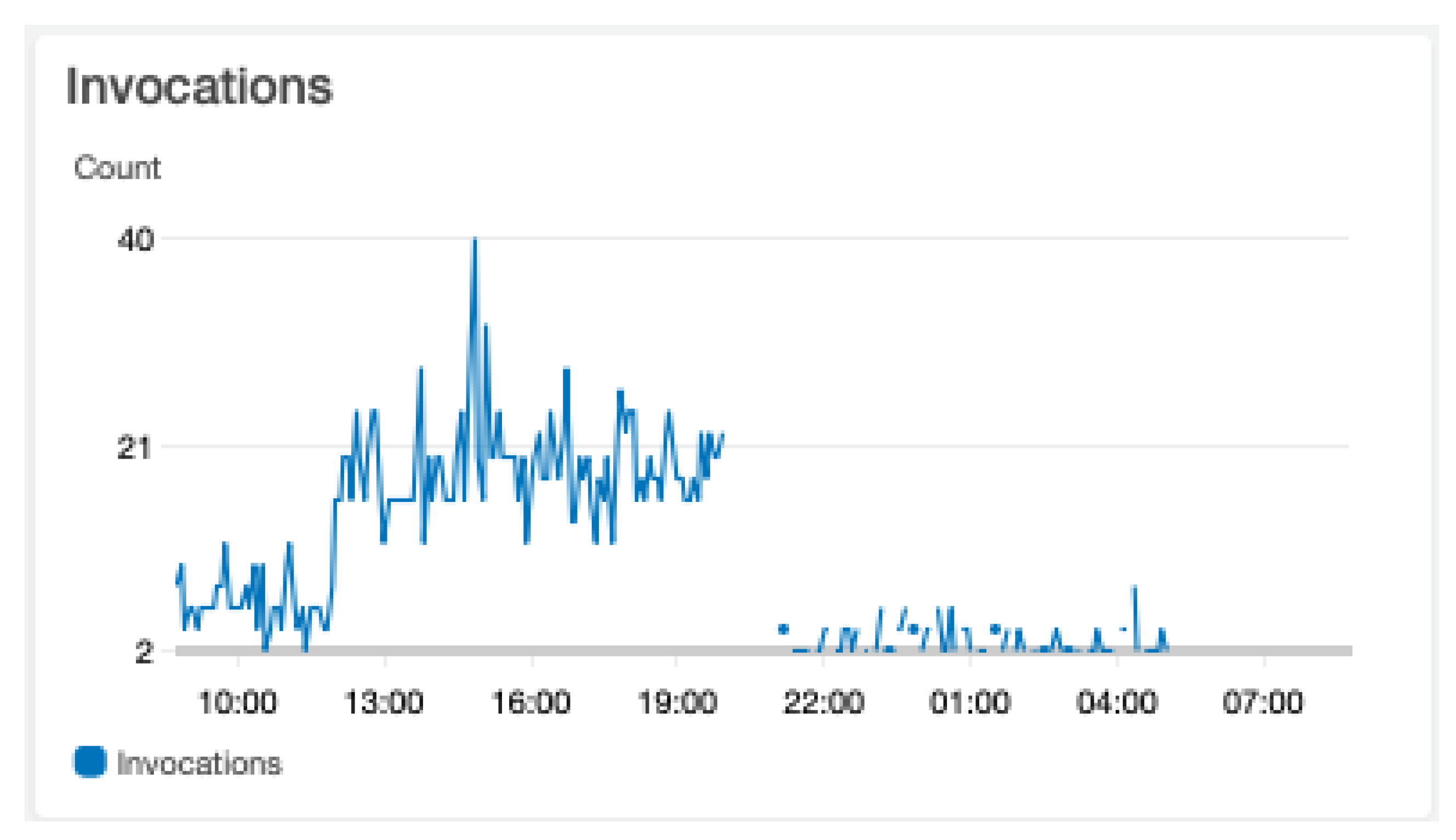
Figure 8.
Concurrency Levels: (upper) Concurrency Interval 1–5; and (lower) Concurrency Interval 6.

Figure 9.
Intervals invocations.

Figure 10.
Interval 1 IP Distribution.

Figure 11.
Interval 2 IP Distribution.

Figure 12.
Interval 3 IP Distribution.

Figure 13.
Interval 4 IP Distribution.

Figure 14.
Interval 5 IP Distribution.
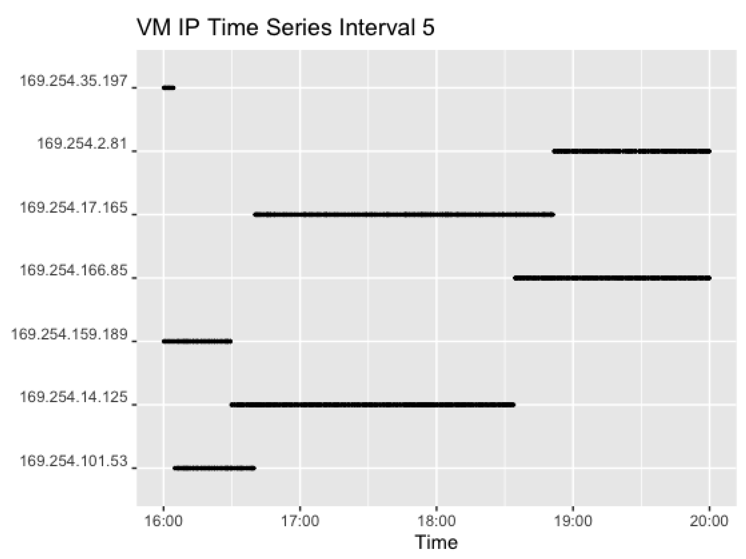
Figure 15.
Interval 6 IP Distribution.

Figure 16.
IP changes of a 5 min request rate interval.

Figure 17.
IP changes of a 1 min and 10 min request rate interval (Hello World function).

Figure 18.
Postman Results for 20 min Run.
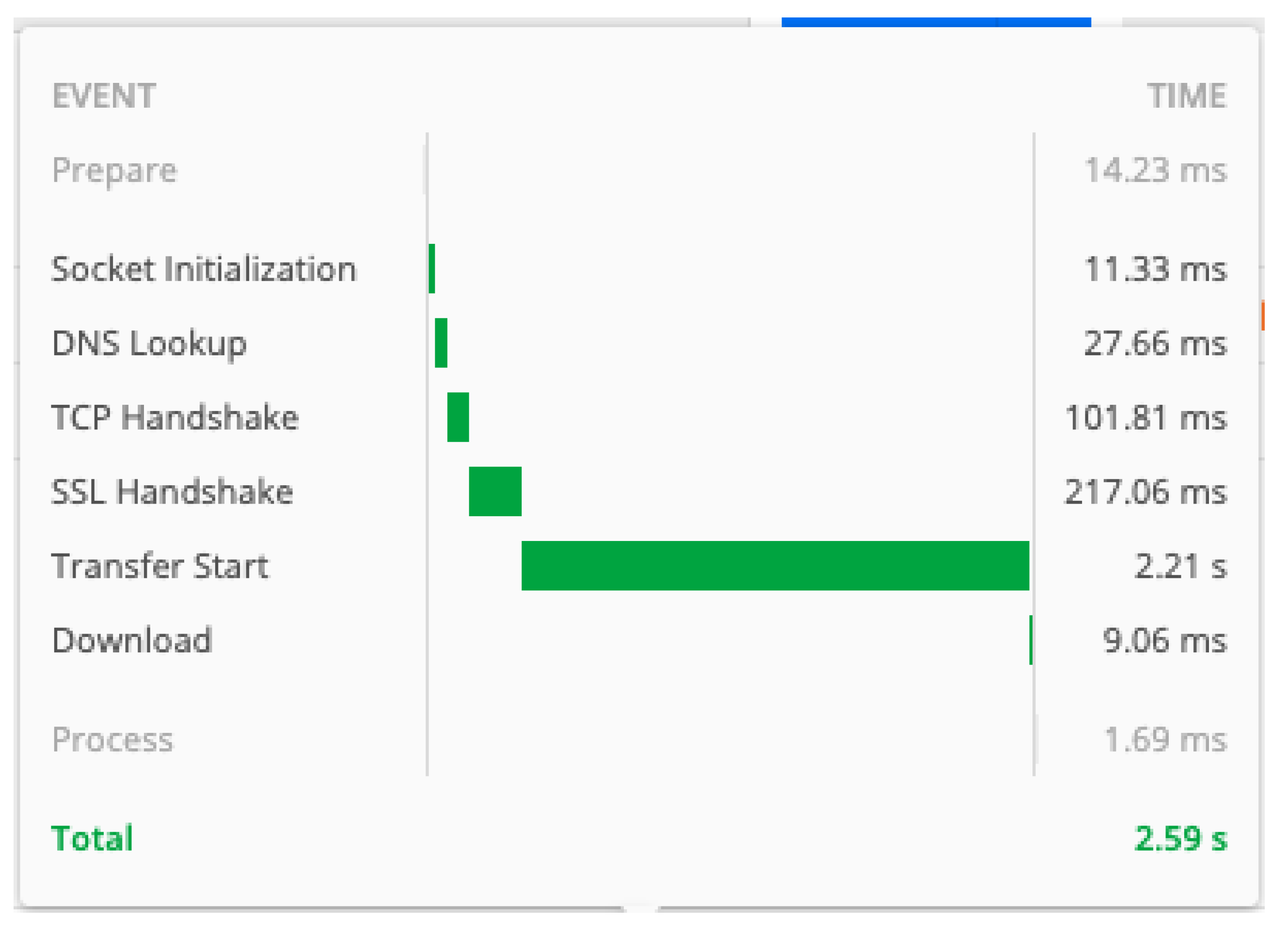
Figure 19.
Postman Test TCP and Round-Trip-Time per Request Rate: Red Line, TCP time (ms); Blue Line, Round-Trip-Time time (ms).
Figure 19.
Postman Test TCP and Round-Trip-Time per Request Rate: Red Line, TCP time (ms); Blue Line, Round-Trip-Time time (ms).


Table 1.
Function instance configurations.
| Memory | 128 MB [ up to 64 * k (k = 2,3, …, 24)] |
| CPU | allocated proportional to memory |
| Max Timeout | 300 ms [up to 900 ms] |
| Runtime Language | Python 3.7 (3.6, 2.7) |
| Billing Specification | execution time allocated on memory |
Table 2.
Descriptive statistics versions.
| Cold-Start Median: | 23,302 ms = 23.3 s |
| min = 22,103 ms | |
| max = 24,645 ms | |
| Round-Trip-Time Median: | 146,306 ms = 146 s |
| Cold-Start Standard Deviation: | 695.28 ms |
Table 3.
Versions mean Cold-Start.
| Version | Mean Cold-Start |
|---|---|
| Python 2.7: | 23,436 ms (Highest) |
| Python 3.6: | 23,309 ms |
| Python 3.7: | 23,216 ms (Lowest) |
Table 4.
Versions mean Round-Trip-Time.
| Version | Mean Round-Trip-Time |
|---|---|
| Python 2.7: | 146,330 ms (Highest) |
| Python 3.6: | 146,280 ms (Lowest) |
| Python 3.7: | 146,314 ms |
Table 5.
Descriptive Statistics File Upload Stream.
| Cold-Start Median: | 23,064 ms = 23 s |
| min = 14,360 ms | |
| max = 21,579 ms | |
| mean = 23,042 ms | |
| Round-Trip-Time Median: | 146,437 ms = 146.46 s |
| min = 146,115 ms | |
| max = 148,021 ms | |
| mean = 146,750 ms | |
| Cold-Start Standard Deviation: | 769.50 ms |
Table 6.
Descriptive Statistics Scale Test.
| Cold-Start Median: | 26,682 ms = 26.68 s |
| min = 25,086 ms | |
| max = 29,312 ms | |
| Round-Trip Time Median: | 151,029 ms = 151 s |
| min = 149,640 ms | |
| max = 153,125 ms | |
| Cold-Start Standard Deviation: | 869.84 ms |
Table 7.
Dataset Extract Re-Used VMs—I.
| Round | Runtime | Memory | FunctionName | InstanceIDGeneratedByFunction | |
|---|---|---|---|---|---|
| 5 | 1 | python2.7 | 3008 | Cold-Start56234411 | 8b381842-ed0f-484a-a2da-c6a8bb9b5646 |
| 8 | 2 | python2.7 | 3008 | Cold-Start56234411 | 8b381842-ed0f-484a-a2da-c6a8bb9b5646 |
| 10 | 1 | Python 3.6 | 128 | Cold-Start56535486 | c47e5160-58c7-460c-bcdb-87699a70fcf5 |
| 12 | 2 | Python 3.6 | 128 | Cold-Start56535486 | c47e5160-58c7-460c-bcdb-87699a70fcf5 |
| 21 | 1 | Python 3.7 | 3008 | Cold-Start57436585 | 970f1644-51cf-4b4b-bafa-4f09303c96ca |
| 24 | 2 | Python 3.7 | 3008 | Cold-Start57436585 | 970f1644-51cf-4b4b-bafa-4f09303c96ca |
Note: the first VM (in red).
Table 8.
Dataset Extract Re-Used VMs—II.
| RequestID | VMid | InstanceID | |
|---|---|---|---|
| 5 | 8b381842-ed0f-484a-a2da-c6a8bb9b5646 | sandbox-root-nZM9qu | sandbox-58ab44 |
| 8 | e2f287ff-0859-4aa8-b964-f850fe417949 | sandbox-root-nZM9qu | sandbox-58ab44 |
| 10 | c47e5160-58c7-460c-bcdb-87699a70fcf5 | sandbox-root-fHvRZn | sandbox-bd9454 |
| 12 | ef6184ba-9b82-445e-b532-ae12a4e2128e | sandbox-root-fHvRZn | sandbox-bd9454 |
| 21 | 970f1644-51cf-4b4b-bafa-4f09303c96ca | sandbox-root-5w4RTV | sandbox-service-c6ed64 |
| 24 | 432d7a53-6f01-4efb-80cd-243ca891c3f0 | sandbox-root-5w4RTV | sandbox-service-c6ed64 |
Note: the first VM (in red).
Table 9.
Dataset Extract Re-Used VMs—III.
| InstanceVMip | PublicVMip | PrivateInstanceIP | ResponseProcessing | RequestRTT | |
|---|---|---|---|---|---|
| 5 | 169.254.96.253 | 3.236.218.254 | 169.254.76.1 | 23,412.49 ms | 146,293.55 ms |
| 8 | 169.254.96.253 | 3.236.218.254 | 169.254.76.1 | 22,143.02 ms | 146,356.15 ms |
| 10 | 169.254.107.125 | 100.24.27.41 | 169.254.76.1 | 22,432.59 ms | 146,361.03 ms |
| 12 | 169.254.107.125 | 100.24.27.41 | 169.254.76.1 | 23,547.74 ms | 146,409.49 ms |
| 21 | 169.254.35.229 | 54.159.6.73 | 169.254.76.1 | 22,801.62 ms | 146,392.74 ms |
| 24 | 169.254.35.229 | 54.159.6.73 | 169.254.76.1 | 22,934.30 ms | 146,348.71 ms |
Note: the first VM (in red); the second instance latency (in blue).
Table 10.
Interval Concurrency and Used IPs.
| Interval | Concurrency | No. of Invocations | No. of IPs used |
|---|---|---|---|
| 1st | 1 | 50 | 1 |
| 2nd | 1 | 54 | 3 |
| 3rd | 2 | 306 | 5 |
| 4th | 4 | 930 | 11 |
| 5th | 2 | 920 | 7 |
| 6th | 2 | 174 | 31 |
Table 11.
Intervals Processor Information VMs.
| Variable | Technical Characteristics |
|---|---|
| Model Name: | GenuineIntel |
| Intel(R) Xeon(R) Processor @ 2.50GHz | |
| Intel(R) Xeon(R) Processor @ 3.00GHz | |
| Model: | 62 |
| CPU family: | 6 |
| CPU MHz: | 2499.994–3000.014 MHz |
| Address Sizes: | 46 bits physical, 48 bits virtual |
| MemTotal: | 192,480 kB |
| MemFree: | 36,700–63,932 kB |
| MemAvailable: | 126,896–141,436 kB |
| Cached: | 71,652–767,72 kB |
Table 12.
Example Cold and Warm Start Request.
| RequestId | ba26617e-4482-43bb-bbe1-d3bec76bd05e |
| Duration: | 401.11 ms |
| Billed Duration: | 500 ms |
| Memory Size: | 128 MB |
| Max Memory Used: | 79 MB |
| RequestId | 45036707-50be-4e19-a4ae-211283d18b60 |
| Duration: | 1862.08 ms |
| Billed Duration: | 1900 ms |
| Memory Size: | 128 MB |
| Memory Used: | 79 MB |
| Init Duration: | 320.53 ms |
Table 13.
Postman Test Settings.
| Pause Time | Round-Trip-Time |
|---|---|
| 20 min | 2.75 s |
| 15 min | 3.10 s |
| 12 min | 2.75 s |
| 10 min | 1.43 s |
| 5 min | 1.03 s |
| 1 min | 0.808 s |
| 1 s | 0.785 s |
Publisher’s Note: MDPI stays neutral with regard to jurisdictional claims in published maps and institutional affiliations. |
© 2020 by the authors. Licensee MDPI, Basel, Switzerland. This article is an open access article distributed under the terms and conditions of the Creative Commons Attribution (CC BY) license (http://creativecommons.org/licenses/by/4.0/).
Share and Cite
MDPI and ACS Style
Muller, L.; Chrysoulas, C.; Pitropakis, N.; Barclay, P.J. A Traffic Analysis on Serverless Computing Based on the Example of a File Upload Stream on AWS Lambda. Big Data Cogn. Comput. 2020, 4, 38. https://doi.org/10.3390/bdcc4040038
AMA Style
Muller L, Chrysoulas C, Pitropakis N, Barclay PJ. A Traffic Analysis on Serverless Computing Based on the Example of a File Upload Stream on AWS Lambda. Big Data and Cognitive Computing. 2020; 4(4):38. https://doi.org/10.3390/bdcc4040038
Chicago/Turabian StyleMuller, Lisa, Christos Chrysoulas, Nikolaos Pitropakis, and Peter J. Barclay. 2020. "A Traffic Analysis on Serverless Computing Based on the Example of a File Upload Stream on AWS Lambda" Big Data and Cognitive Computing 4, no. 4: 38. https://doi.org/10.3390/bdcc4040038