USRT: A Solar Radiative Transfer Model Dedicated to Estimating Urban 3D Surface Reflectance

1
College of Resource Environment and Tourism, Capital Normal University, Beijing 100048, China
2
Beijing Laboratory of Water Resources Security, Beijing 100048, China
*
Author to whom correspondence should be addressed.
Urban Sci. 2020, 4(4), 66; https://doi.org/10.3390/urbansci4040066
Submission received: 22 September 2020
/
Revised: 18 November 2020
/
Accepted: 25 November 2020
/
Published: 27 November 2020
Abstract
:Urban 3D surface reflectance is a critical parameter for the modeling of surface biophysical processes. It is of great significance to enhance the accuracy of reflectance in urban areas. Based on the urban solar radiative transfer (USRT) model, this study presents a methodology for estimating urban reflectance using the sky view factor (SVF) derived from airborne LiDAR data. Then, the USRT model was used to retrieve urban 3D surface reflectance from Landsat 8 data over the typical area of Beijing. The reflectance from USRT model was compared with the estimated value obtained from the model without considering the impact of morphological characteristics of the urban underlying surface (flat model). The results showed that the urban sample reflectance estimated by the USRT model was close to the sample reflectance of the suburban underlying surface which was less affected by morphological characteristics. The research summaries are as follows: (1) The definite physical meaning is presented in the USRT model, and can be applied to estimate the physical parameters of the urban underlying surface. (2) The reflectance from the USRT model is slightly larger than the reflectance derived from the flat model, which indicates that the accuracy of urban 3D surface reflectance is improved by the USRT model. (3) The effects of the SVF and building reflectance are different. The SVF presents a strong sensitivity to the estimation of the urban 3D surface reflectance, and the variations of building reflectance setting have little impact on urban reflectance, which is characterized by low sensitivity. Generally, the methodology of estimating urban reflectance proposed in this study can better clarify the impact mechanism of urban geometry on the radiative transfer processes and further promote the application and development of urban quantitative remote sensing.
1. Introduction
The urban 3D surface reflectance, representing the reflective ability of urban surface objects to solar radiation, affects the quantitative retrieval of surface biophysical parameters and the accurate modeling of the surface energy balance. Resulting from the rapid development of remote sensing satellites and platforms, remote sensing data can be increasingly used for retrieval of urban 3D surface reflectance. However, there is still a challenge for calculation of urban reflectance, because the morphological and structural characteristics of the urban underlying surface are rarely considered in current radiative transfer models [1,2,3]. Most of the radiative transfer models are based on the assumption that the urban land surface is a horizontal surface, but the geometry of urban areas is always complex in the real world. The spectral radiance recorded by a sensor is an integrated result of solar radiation with the earth’s atmosphere and urban surface [4,5,6]. The solar incident radiation received by a pixel has been regulated due to the impact of urban morphological characteristics, and, thus, the information of urban surfaces is distorted. Therefore, careful modeling of each component in the radiative transfer model is required to accurately calculate the results of urban 3D surface reflectance. In order to obtain the urban reflectance with promising accuracy, there is an urgent need to construct a radiative transfer model considering the urban geometrical characteristics. Constructing a reasonable radiative transfer model suitable for urban areas is of great importance for applications of surface reflectance retrieval, as well as the development of current quantitative remote sensing field in urban areas.
In recent years, much attention has been paid to the effects of surface heterogeneity on the solar radiative transfer processes [7,8], among which two sceneries are discussed mostly: mountainous and vegetation areas [9,10,11,12,13,14]. For example, Wen et al. (2008) proposed a model for topographic correction to improve the accuracy of surface reflectance in the terrain area, with coupling the influence of mountain radiation transmission and terrain multiple scattering [12]. Wang and Li (2013) developed a multiple-layer canopy radiative transfer model (MRTM) to calculate vegetation canopy reflectance, which separated the roles of incident direct and diffuse radiation and radiation singly and multiply scattered by foliage [14]. However, they cannot be applied to complex urban scenarios. Chen et al. (2013) proposed a novel method for empirical reflectance retrieval in urban environments that is applicable to both sunlit and shadowed regions [15]. In contrast, the urban–atmosphere coupling term and the multiple reflections were still roughly modelled in this study. With the great progresses of theoretical foundation of radiative transfer processes and space technology in launching more and more high spatial- and temporal-resolution satellite instruments, an improved understanding of quantitative description of 3-dimensional morphological characteristics over urban regions is attracting increasing interest of the remote sensing community, which also makes the forward modeling of urban heterogeneous surface available [7,16,17,18].
Three-dimensional morphological characteristics formed by urban longitudinal extension are one of the main factors affecting the incident radiation transmission over urban regions [19,20,21,22]. Selection of surface parameters that can represent the 3-dimensional morphological characteristics of urban areas is critical to the modeling of urban radiative transfer processes. At present, the parameters used to depict the urban geometric characteristics mainly include building height, building density, the planar area index (PAI), the frontal area index (FAI), the height/width ratio (H/W), and the sky view factor (SVF) [23,24,25,26]. The SVF is commonly used to indicate the openness of a particular area within an urban setting and in general a terrestrial landscape [27,28], and can also be used as an indicator representing combinations of other parameters such as building height and building density [27]. It is one of the most concerned urban morphological parameters, and has been widely used in the study of urban heat island effect [29], urban energy balance [30], urban land surface temperature [31], and many successful cases in exploring the impact of urban 3-dimensional geometric structures on the urban microclimate [31,32,33]. These studies indicate that the SVF can be utilized to parameterize the effect of urban geometry on climate. Hence, the SVF could be considered as a key dominant factor in the construction of radiative transfer model over urban areas.
In this study, the SVF was introduced to establish a radiative transfer model for the urban scene, the urban solar radiative transfer (USRT) model. Additionally, the USRT model was used to retrieve urban 3D surface reflectance from Landsat 8 data over the typical area of Beijing. Then, the retrieval ability of the USRT model to urban 3D surface reflectance is illustrated from the following three aspects: (1) validation of reflectance results estimated by the USRT model, (2) the comparison of the reflectance calculated by the USRT model and the flat model, and (3) sensitivity analysis of core surface parameters in the USRT model.
2. Principle and Method
2.1. Description of the USRT Model
The USRT model is an urban radiative transfer model for the reflective spectral domain (0.4–2.5 μm), proceeding by identifying the irradiance components at each point of the landscape and the radiance components reaching a satellite—or airborne sensor, and then computing them separately. The USRT model was based on radiative transfer equation and was designed according to ideas proposed in papers [10,12]. The assumption and simplification of the urban underlying surface are the foundation of constructing an urban radiative transfer model. Therefore, the USRT model was established by assuming the following two conditions: (1) regular buildings stand on a flat surface, and (2) the ground and building surface are Lambertian surface. On this basis, the impact of urban structural and morphological characteristics on the solar radiative transfer process is mainly described in three aspects: (1) the solar direct radiation may not reach target pixel because of the blocking of buildings, (2) the sky diffuse radiation received by the target pixel is changed by the urban geometry, and (3) the vertical facets of buildings can reflect the solar radiation to the target pixel, and complex geometry of built-up areas increases multiple scattering within the urban canopy. The sky view factor is used to quantify the sky diffuse radiation and multiple scattering processes in the USRT model.
2.1.1. The Total Radiation Received by the Target Pixel
Considering a sensor observing an urban scene and P a pixel of the remote sensing image, the total irradiance, , received by the target pixel (P) of the urban scene can be calculated as follows:
where is the solar direct irradiance (), is the sky diffuse irradiance (), and is the reflected irradiance ().
(1)
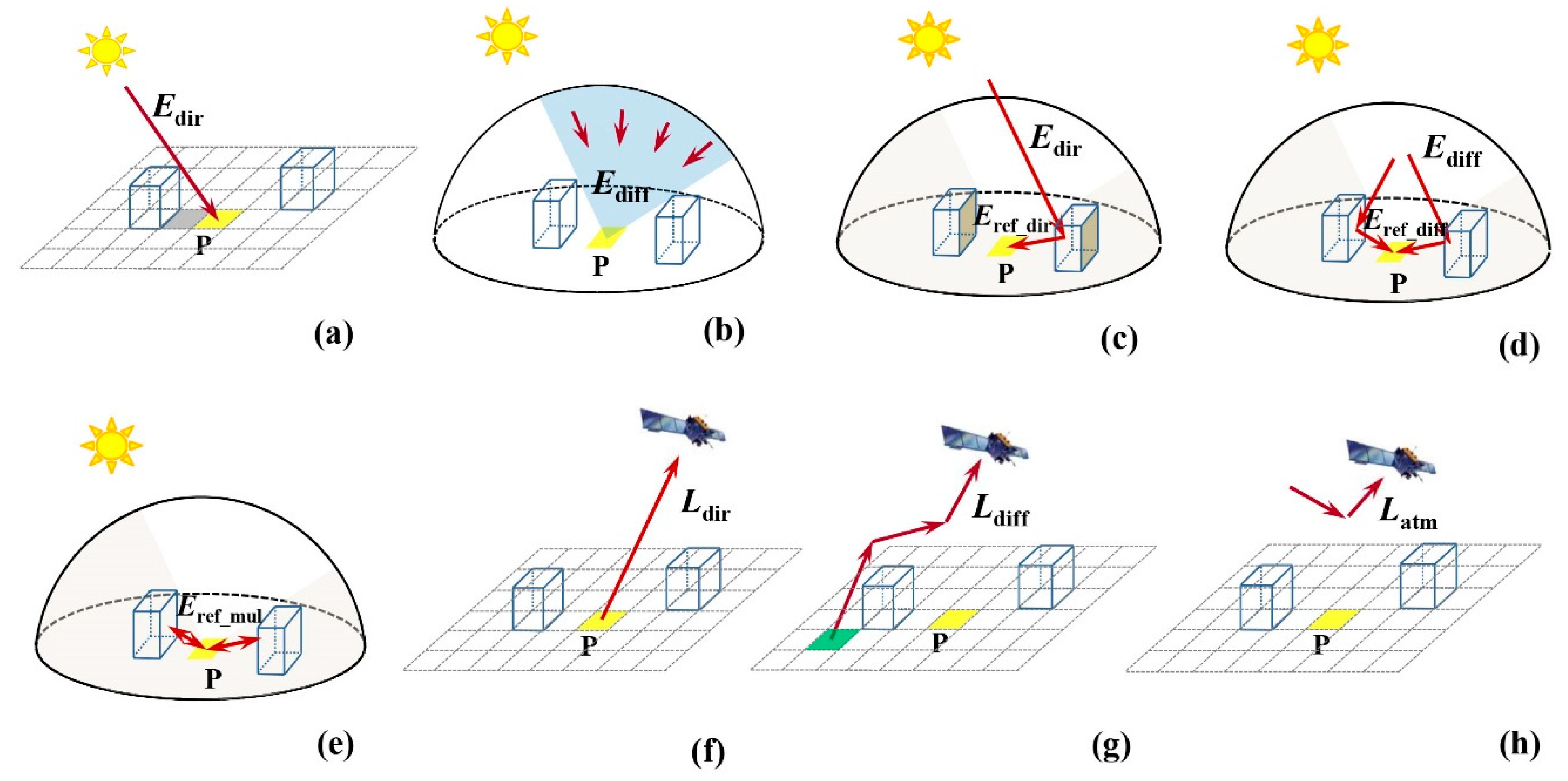
Downward solar direct radiation () corresponds to photons coming directly from the sun and transmitting to the urban scene. However, this component may not be received by the target pixel due to the blocking of urban buildings (Figure 1a). The yellow area in Figure 1 represents the target pixel, and the black area in Figure 1a represents the shadow caused by the occlusion of tall buildings. Therefore, can be expressed as follows [10]:
where is the exo-atmospheric irradiance (), and is a binary coefficient which is set to zero to indicate that a pixel is not illuminated by the sun and set to one otherwise. is the atmospheric transmittance of direct downward solar radiation. is the solar zenith angle.
(2)
The component models the photons scattered by the atmosphere to the ground. The sky diffuse irradiance will be reduced when the sky dome overlying the surface is not an integrated hemisphere of a horizontal surface. The target pixel can only receive the diffuse irradiance within the visible range of the sky (Figure 1b). can be quantified with the sky view factor (SVF) as follows:
where is the downward diffuse transmittance. is sky view factor defined as the ratio of the irradiance on a specific surface to that on an unobstructed horizontal surface, and, obviously, the value of is between 0 and 1.
(3)
The components correspond to the irradiances depending on the neighboring environment that are the results of the reflections of the buildings around the target pixel. The reflected irradiance mainly consists of three parts: (1) the component corresponding to the irradiance coming from solar direct irradiance received and reflected by the vertical facets of buildings (Figure 1c); (2) the component corresponding to the irradiance coming from sky diffuse irradiance received and reflected by the vertical facets of buildings (Figure 1d); and (3) the component, which can be modeled as multiple reflections between target objects and the vertical facets of buildings (Figure 1e). The expression is as follows:
where is the building reflectance. It is worth noting that only the direction facing the sun can receive the direct solar radiation in the urban scene due to the directivity of solar radiation.
Then, the radiation is reflected by the urban surface after reaching the target pixel. After m-times reflections between the target pixel and vertical facets of buildings, the multiple reflected irradiance () received by the target pixel can be formulated as an equal ratio sequence:
where is the urban 3D surface reflectance. When m tends to infinity, Equation (6) can be simplified as:
Therefore, the total reflected irradiance () received by the target pixel can be quantified as follows:
Finally, combining Equation (2) to Equation (8), the total irradiance () received by the target pixel in urban scene can be written as Equation (9):
2.1.2. The Radiance Reaching the Sensor
The radiance reaching to the satellite can be quantified as follows:
where is the radiance of top of atmosphere (), is the radiance of target pixel reaching the satellite (), is the diffuse radiance of surrounding pixel reaching the satellite (), and is the path radiance ().
(1)
The radiance reflected by the surface to the sensor can be expressed as follows (Figure 1f):
where is the total solar irradiance received by the target pixel (), and is the atmospheric transmittance of upward radiation.
(2)
The radiation reflected by the surrounding target may also reach the sensor by atmospheric scattering (Figure 1g). The green area in Figure 1f represents the surrounding pixel. The upward diffuse radiance of surrounding target can be modeled as
where is the upward diffuse transmittance.
(3)
The path radiance reaching the sensor can be modeled as (Figure 1h)
where is the atmospheric reflectance.
According to Equation (11) to Equation (13), the radiance reaching the satellite can be written as follows:
where is the upward total transmittance, and .
2.2. Reflectance Calculation Model Based on the USRT Model
According to Equations (9) and (14), the reflectance of the urban underlying surface can be expressed as follows:
In Equation (15), building reflectance () and the SVF () are the two critical input parameters for accurate reflectance estimation. In addition, the at-satellite radiance is obtained by remote sensing imagery. Other solar radiation and atmospheric parameters can be simulated by the 6S model, including exo-atmospheric irradiance (), path radiance (), atmospheric transmittance of downward solar direct radiation (), downward diffuse transmittance (), and upward total transmittance ().
3. Study Area and Data
3.1. Study Area
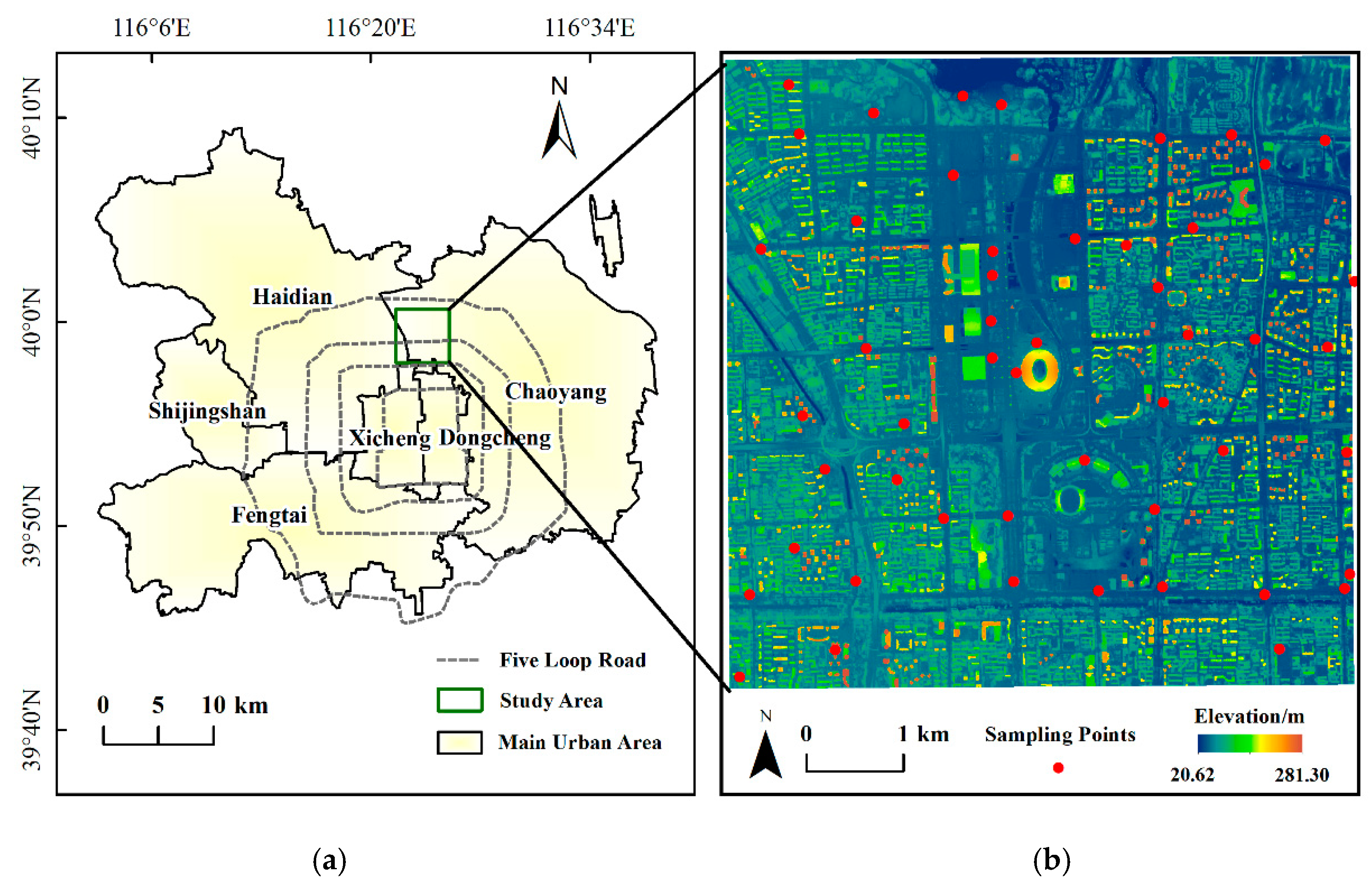
The study site is located at the junction of Haidian District and Chaoyang District, Beijing, between the north fourth loop road and the north fifth loop road. The study area covers approximately 25 km2 (Figure 2), which is composed of some construction facilities (e.g., National Stadium, National Indoor Stadium, etc.) and part of the Olympic park. The terrain is relatively flat, and the main land use/cover types include buildings, roads, trees, water, and bare land. In general, buildings of this study area have the combined characteristics of different heights and densities, which are suitable for carrying out the research of remote sensing retrieval of urban reflectance.
3.2. Data
In this research, the Landsat 8 satellite data, airborne LiDAR data, and field measured data were used. Landsat 8 satellite data were downloaded from the United States Geological Survey (USGS, https://earthexplorer.usgs.gov). Landsat OLI (Operational Land Imager) data were acquired under clear atmospheric conditions on 27 June 2018, including blue, green, and red bands. The orbit number and spatial resolutions of the imagery were path 123/row 32 and 30 m, respectively.
Airborne LiDAR data were obtained from the airborne Leica ALS 60system, with the point cloud density of about 2–4 points/m2. The LiDAR data were interpolated to obtain DSM (digital surface model) data, with the spatial resolution of 0.5 m (Figure 2b).
In order to evaluate the accuracy of the SVF, a fisheye camera was used to measure the SVF in the study area. 48 fisheye pictures were taken in different building density and height areas to collect various types of SVF. To ensure the reliability of the collected data, the sampling points were evenly distributed in the study area (Figure 2b). The fisheye lens used sigma 8 mm f3.5 ex DG fisheye, and its viewing angle range could reach 180°, which was suitable for quantitative analysis of sky view range.
4. Data Processing and Result Analysis
4.1. Results and Analysis of the SVF
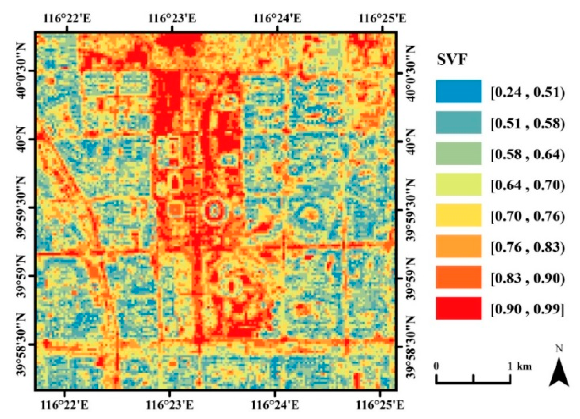
DSM was generated by airborne LiDAR data, and more details on the estimation of the SVF can be found in [34]. In this paper, Zakšek et al. (2011) proposed a method to calculate the SVF by introducing a solid angle. The solid angle of an object is proportional to area of the object’s projection onto the unity sphere centered at the observation point. If the horizon is not of equal height in all directions, the solid angle can be computed by observing the horizon vertical elevation angle in a chosen number of directions, and then values of the SVF within the study area can be obtained. In Zakšek’s method, the field measured data of the fisheye lens were used as the validation data to set optimal search directions and the search radius. Thirty-two directions and a search radius of 80 pixels were chosen to estimate the SVF in this study [35]. In order to match the analysis scale of the USRT model, the raster of the SVF was resampled to 30 m. The SVF was divided into eight levels according to the method of Jenks’ natural breaks (Figure 3). The proportion of the SVF in each level was 5.163%, 12.558%, 17.580%, 16.351%, 15.282%, 13.713%, 11.150% and 8.204%, respectively.
The SVF is the critical indicator of describing the morphological characteristics of the urban underlying surface, and the other parameters used to depict the urban geometric characteristics also include building height and building density [32,36,37,38]. Therefore, the availability of the SVF derived from airborne LiDAR data could be evaluated by analyzing the correlation between the SVF and building indicators (i.e., building height and building density). Based on the obtained building data, the average building height and building density within each SVF zone were calculated, and eight sets of values were acquired, respectively. Figure 4 showed the relationship between the SVF and building height and building density, respectively. The results indicated that the SVF had a positive correlation with building height and building density, and the goodness of fit (R2) was 0.95 and 0.88, respectively. Therefore, the morphological characteristics of the underlying surface can be well expressed by the SVF.
4.2. Results and Analysis of Urban 3D Surface Reflectance
The determination of the SVF is described in Section 4.1. The building reflectance was set to 0.3, and the sensitivity analysis of this parameter will be described in detail in the Discussion Section. Other parameters were derived from the 6S model, and the simulation results are shown in Table 1. Urban 3D surface reflectance was obtained by substituting the SVF, building reflectance, solar radiative parameters and atmospheric parameters into Equation (12) (Figure 5). The average of urban reflectance in blue, green and red bands under different SVFs were calculated, as shown in Table 2.
On the whole, the average reflectance of blue, green, and red band was 0.133, 0.150, and 0.143, respectively. The urban 3D surface reflectance varied with different SVFs in the three bands, which indicated that the SVF had a certain impact on the remote sensing retrieval of urban 3D surface reflectance. In addition, it is necessary to consider the morphological characteristics of the urban area when estimating the urban 3D surface reflectance.
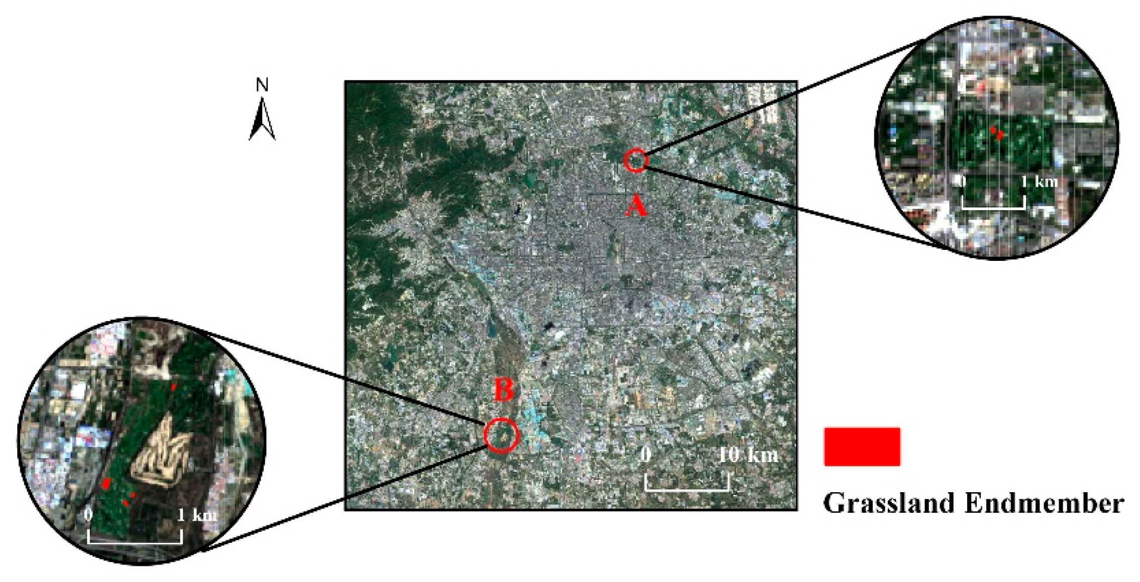
The reflectance values of the natural materials are material characteristic property, that is, reflectance of the same natural material is invariant theoretically in both urban and suburban regions. In order to verify the positive role of the USRT model in the remote sensing retrieval of urban 3D surface reflectance, pure grassland pixels of the urban area (i.e., study area) and suburban area were selected in this study for comparison, as shown in Figure 6. Buildings may have a certain visual shielding effect on the urban surfaces. The radiative transfer processes in urban areas were strongly affected by surrounding buildings, while the impact of buildings on the radiative transfer processes could be neglected due to the flat terrain and a few buildings in the selected suburban area. The role of the USRT model on reflectance retrieval could be explained by analyzing the reflectance of the same land use/cover type.
The pure grassland pixels selected in urban and suburban areas are shown in Figure 6, where A is in the urban area and B is in a suburban area. Two models were used to retrieve reflectance of grassland in urban area and suburban area, respectively. One is the USRT model, and the other is the model without considering the urban morphological characteristics, which was named the “flat model” in this paper. Table 3 showed the comparison analysis of pure grassland pixels’ reflectance derived from the two models in urban and suburban area. Results indicated that: (1) urban grassland reflectance estimated by the USRT model was larger than the results of the flat model; (2) the reflectance of urban samples retrieved by the USRT model was closer to the reflectance of suburban samples derived from the flat model, which illustrated that the USRT model improved the accuracy of urban 3D surface reflectance, and the radiative transfer model constructed for the urban underlying surface had a positive effect on the accurate retrieval of surface reflectance.
In Table 3, the morphological characteristics of urban areas were taken into account in the USRT model, while the flat model assumed the urban underlying surface as a horizontal surface. The main differences between the two models were as follows: (1) the flat model assumed that the earth surface received all direct solar radiation, while the USRT model took into account the blocking of direct solar radiation by buildings and used the binary coefficient to quantify; (2) morphological and structural characteristics were neglected in the flat model to quantify the sky diffuse radiation and environmental radiation, while the SVF was used in the USRT model to quantify the sky diffuse radiation reaching the urban surface and multiple scattering between target object and vertical facets of buildings.
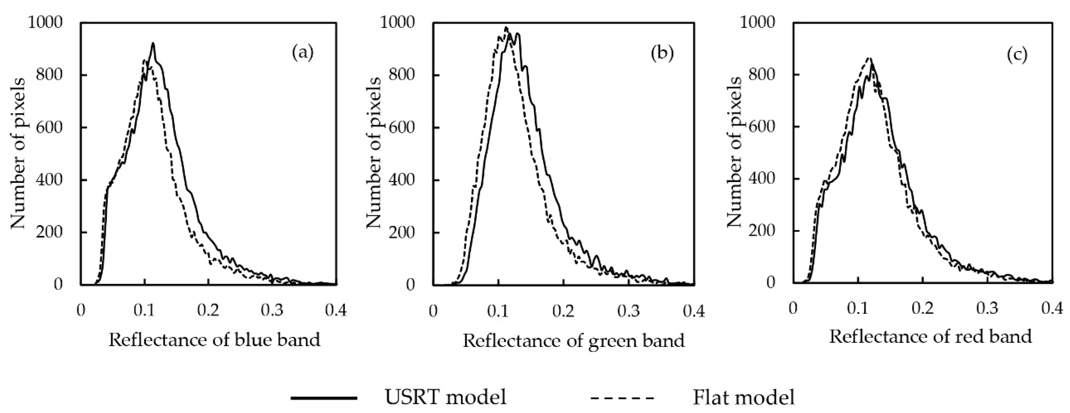
The graphs of urban reflectance in the whole study area derived from the two models are shown in Figure 7. The results illustrated the following: (1) The reflectance from the USRT model was slightly higher than the results of the flat model. This was mainly because the impact of the SVF and interception effect on the incident radiation were taken into account in the USRT model, which could improve the accuracy of urban 3D surface reflectance. (2) Wavelength was also one of the factors affecting reflectance. For Landsat 8 multispectral data, the difference between the results of the two models gradually narrowed with the increase in wavelength from the blue to red band.
5. Discussion
5.1. The Impact of the SVF on Urban 3D Surface Reflectance
The SVF is a critical parameter to describe the morphological characteristics of the urban underlying surface, which is the main driving factor of the USRT model [20]. Sensitivity analysis of the SVF is of great significance to enrich the modeling of urban radiative transfer and improve the accuracy of the model.
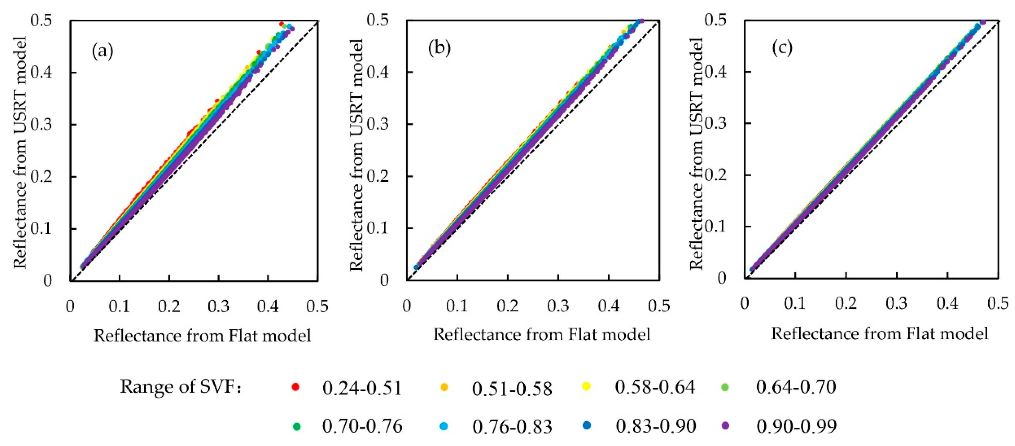
The impact of the morphological characteristics parameter (SVF) on urban reflectance is revealed in Figure 8. The results illustrated the following: (1) the reflectance from the USRT model was consistent with the reflectance from the flat model; (2) urban 3D surface reflectance was decreasing with the SVF increasing and the value was closer to the reflectance derived from the flat model. This was mainly because the urban surface was closer to flat surface with the increasing SVF.
5.2. The Impcat of Building Reflectance on Urban 3D Surface Reflectance
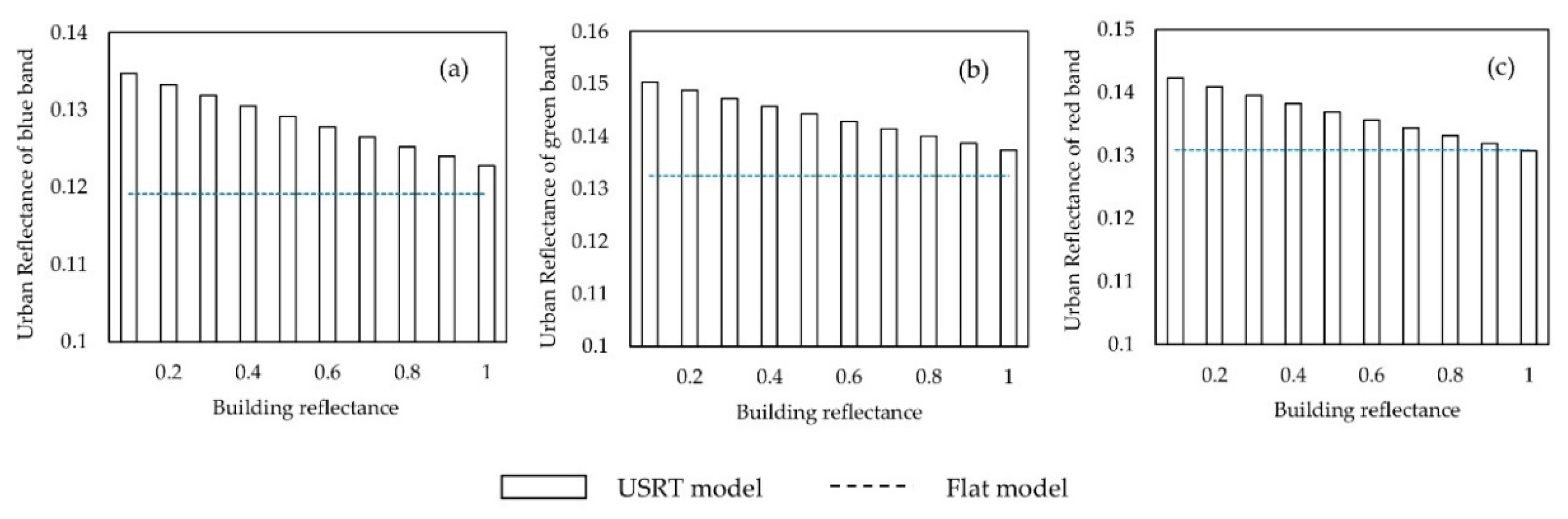
The impact analysis of building reflectance on urban 3D surface reflectance was conducted in this study where the building reflectance was limited to a range from 0 to 1 with the change step of 0.1 (Figure 9). The results indicated the following: (1) urban 3D surface reflectance was decreasing in each band with increasing building reflectance; (2) the reflectance of the urban underlying surface from the USRT model was higher than the reflectance obtained from the flat model within the range of building reflectance; (3) the variation of building reflectance had little impact on urban reflectance, where the urban reflectance of blue, green, red band was limited to a range of from 0.12 to 0.13, 0.14 to 0.15, 0.13 to 0.14, respectively. The variation of building reflectance only brought about a fluctuation of 0.01 on the value of urban 3D surface reflectance.
Hence, the USRT model can weaken the impact of parameter setting of building reflectance on the radiative transfer processes and effectively amplify the influence of surface morphological parameter (i.e., the SVF) on the radiative transfer processes. Notably, a single parameter analysis method was used in sensitivity analysis, i.e., setting a reasonable change step and considering the mutual independence of parameters. In fact, although the parameters are not completely independent, the incomplete independence will not affect the research conclusion in essence.
6. Summaries
In this study, an urban solar radiative transfer model (i.e., USRT model) operating in the visible and short wave infrared was presented. The objective of the study was to develop an urban radiative transfer model able to deal with the problem of the remote sensing retrieval of reflectance over urban areas. To solve this inverse problem, irradiance and radiance components were modelled separately. The conclusions are as follows:
(1) The USRT model modelled separately the irradiance and radiance components at ground and sensor level, and each component took into account the relief, ground heterogeneity and atmospheric corrections. The physical meaning of the USRT model is clear, which can better represent the impact of urban morphological and structural characteristics on incident radiation.
(2) The USRT model has a positive role in improving the accuracy of remote sensing retrieval of urban 3D surface reflectance, by comparing the reflectance of pure pixels on urban and suburban areas.
(3) The SVF and building reflectance have different effects on the reflectance retrieval of the urban underlying surface. The SVF presents a strong sensitivity, while the building reflectance has little impact on the urban 3D surface reflectance, that is, it brings about a fluctuation of 0.01 on the value.
However, the SVF is not the only morphological parameter affecting the urban reflectance, and the contribution of other parameters such as building height and building density should also be taken into account in future research. The effect of the USRT model on the incident radiative transfer processes becomes extremely compatible in the scene of high-rise and high-density buildings, which need to be further analyzed in the near future. Elaborating the applicability of the USRT model in detail is also our research direction in the following study. The USRT model is theoretically applicable to the medium–high-resolution remote sensing image of the urban underlying surface, which can promote the further development of urban quantitative remote sensing.
Author Contributions
Conceptualization, D.H. and M.L.; methodology, D.H., M.L., Y.D., C.Y. and Y.W.; software, M.L.; validation, D.H. and M.L.; formal analysis, D.H. and M.L.; resources, D.H.; data curation, M.L., Y.D., C.Y. and Y.W.; writing—original draft preparation, M.L.; writing—review and editing, D.H.; project administration, D.H.; funding acquisition, D.H. All authors have read and agreed to the published version of the manuscript.
Funding
This research was funded by the National Natural Science Foundation of China under Grant No.41671339, and the projects of Beijing Advanced Innovation Center for Future Urban Design, Beijing University of Civil Engineering and Architecture under Grant No. UDC2019031321.
Conflicts of Interest
The authors declare no conflict of interest.
References
- Bonczak, B.; Kontokosta, C.E. Large-scale parameterization of 3D building morphology in complex urban landscapes using aerial LiDAR and city administrative data. Comput. Environ. Urban Syst. 2019, 73, 126–142. [Google Scholar] [CrossRef]
- Yang, J.; Wong, M.; Menenti, M.; Nichol, J. Modeling the effective emissivity of the urban canopy using sky view factor. ISPRS-J. Photogramm. Remote Sens. 2015, 105, 211–219. [Google Scholar] [CrossRef]
- Gál, T.; Unger, J. A new software tool for SVF calculations using building and tree-crown databases. Urban Clim. 2014, 10, 594–606. [Google Scholar] [CrossRef] [Green Version]
- Cai, G.; Liu, Y.; Du, M. Impact of the 2008 Olympic Games on urban thermal environment in Beijing, China from satellite images. Sustain. Cities Soc. 2017, 32, 212–225. [Google Scholar] [CrossRef]
- Park, C.; Schade, G.W.; Werner, N.D.; Sailor, D.J.; Kim, C. Comparative estimates of anthropogenic heat emission in relation to surface energy balance of a subtropical urban neighborhood. Atmos. Environ. 2016, 126, 182–191. [Google Scholar] [CrossRef] [Green Version]
- Zhou, Y.; Weng, Q.; Gurney, K.R.; Shuai, Y.; Hu, X. Estimation of the relationship between remotely sensed anthropogenic heat discharge and building energy use. ISPRS-J. Photogramm. Remote Sens. 2012, 67, 65–72. [Google Scholar] [CrossRef] [Green Version]
- Liu, Q.; Cao, B.; Zeng, Y.; Li, J.; Du, Y.; Wen, J.; Fan, W.; Zhao, J.; Yang, L. Recent progress on the remote sensing radiative transfer modeling over heterogeneous vegetation canopy. J. Remote Sens. 2016, 20, 933–945. [Google Scholar]
- Wang, K.; Dickinson, R.E. Contribution of solar radiation to decadal temperature variability over land. Proc. Natl. Acad. Sci. USA 2013, 110, 14877–14882. [Google Scholar] [CrossRef] [PubMed] [Green Version]
- Wu, S.; Wen, J.; Gastellu-Etchegorry, J.; Liu, Q.; You, D.; Xiao, Q.; Hao, D.; Lin, X.; Yin, T. The definition of remotely sensed reflectance quantities suitable for rugged terrain. Remote Sens. Environ. 2019, 225, 403–415. [Google Scholar] [CrossRef]
- Wen, J.; Liu, Q.; Xiao, Q.; Liu, Q.; You, D.; Hao, D.; Wu, S.; Lin, X. Characterizing land surface anisotropic reflectance over rugged terrain: A review of concepts and recent developments. Remote Sens. 2018, 10, 370. [Google Scholar] [CrossRef] [Green Version]
- Wen, J.; Liu, Q.; Tang, Y.; Dou, B.; You, D.; Xiao, Q.; Liu, Q. Modeling land surface reflectance coupled BRDF for HJ-1/CCD data of rugged terrain in Heihe river basin, China. IEEE J. Sel. Top. Appl. Earth Obs. Remote Sens. 2015, 8, 1506–1518. [Google Scholar] [CrossRef]
- Wen, J.; Liu, Q.; Xiao, Q.; Liu, Q.; Li, X. Modeling the land surface reflectance for optical remote sensing data in rugged terrain. Sci. China Ser. D Earth Sci. 2008, 51, 1169–1178. [Google Scholar] [CrossRef]
- Mousivand, A.; Verhoef, W.; Menenti, M.; Gorte, B. Modeling top of atmosphere radiance over heterogeneous non-lambertian rugged terrain. Remote Sens. 2015, 7, 8019–8044. [Google Scholar] [CrossRef] [Green Version]
- Wang, Q.; Li, P. Canopy vertical heterogeneity plays a critical role in reflectance simulation. Agric. For. Meteorol. 2013, 169, 111–121. [Google Scholar] [CrossRef]
- Chen, M.; Seow, K.L.C.; Briottet, X.; Pang, S.K. Efficient empirical reflectance retrieval in urban environments. IEEE J. Sel. Top. Appl. Earth Obs. Remote Sens. 2013, 6, 1596–1601. [Google Scholar] [CrossRef]
- Yi, C.; Zhang, Y.; Wu, Q.; Xu, Y.; Remil, O.; Wei, M.; Wang, J. Urban building reconstruction from raw LiDAR point data. Comput.-Aided Des. 2017, 93, 1–14. [Google Scholar] [CrossRef]
- Zeng, Y.; Li, J.; Liu, Q.; Huete, A.; Yin, G.; Xu, B.; Fan, W.; Zhao, J.; Yan, K.; Mu, X. A radiative transfer model for heterogeneous agro-forestry scenarios. IEEE Trans. Geosci. Remote Sens. 2016, 54, 4613–4628. [Google Scholar] [CrossRef]
- Gonzalez-Aguilera, D.; Crespo-Matellan, E.; Hernandez, L.D.; Rodríguez-Gonzálvez, P. Automated urban analysis based on lidar-derived building models. IEEE Trans. Geosci. Remote Sens. 2013, 51, 1844–1851. [Google Scholar] [CrossRef]
- Machete, R.; Falcão, A.P.; Gomes, M.G.; Rodrigues, A.M. The use of 3d GIS to analyse the influence of urban context on buildings’ solar energy potential. Energy Build. 2018, 177, 290–302. [Google Scholar] [CrossRef]
- Overby, M.; Willemsen, P.; Bailey, B.N.; Halverson, S.; Pardyjak, E.R. A rapid and scalable radiation transfer model for complex urban domains. Urban Clim. 2016, 15, 24–44. [Google Scholar] [CrossRef] [Green Version]
- Best, M.J.; Grimmond, C.S.B. Analysis of the seasonal cycle within the first international urban land-surface model comparison. Bound.-Layer Meteor. 2013, 146, 421–446. [Google Scholar] [CrossRef]
- Zhu, S.; Guan, H.; Bennett, J.; Clay, R.; Ewenz, C.; Benger, S.N.; Maghrabi, A.H.; Millington, A. Influence of sky temperature distribution on sky view factor and its applications in urban heat island. Int. J. Climatol. 2013, 33, 1837–1843. [Google Scholar] [CrossRef]
- Wang, Y.; Akbari, H. Effect of sky view factor on outdoor temperature and comfort in Montreal. Environ. Eng. Sci. 2014, 31, 272–287. [Google Scholar] [CrossRef]
- Yang, F.; Qian, F.; Lau, S.S.Y. Urban form and density as indicators for summertime outdoor ventilation potential: A case study on high-rise housing in Shanghai. Build. Environ. 2013, 70, 122–137. [Google Scholar] [CrossRef]
- Cai, Z.; Han, G. Assessing land surface temperature in the mountain city with different urban spatial form based on local climate zone scheme. Mt. Res. 2018, 36, 617–627. [Google Scholar]
- Zhang, H.; Zhu, S.; Gao, Y.; Zhang, G. The relationship between urban spatial morphology parameters and urban heat island intensity under fine weather condition. J. Appl. Meteorol. Sci. 2016, 27, 249–256. [Google Scholar]
- Grimmond, C.S.B.; Potter, S.K.; Zutter, H.N.; Souch, C. Rapid methods to estimate sky-view factors applied to urban areas. Int. J. Climatol. 2001, 21, 903–913. [Google Scholar] [CrossRef]
- Brown, M.J.; Grimmond, S.; Ratti, C. Comparison of Methodologies for Computing Sky View Factor in Urban Environments; Internal Report Los Alamos National Laboratory: Los Alamos, NM, USA, 2001. [Google Scholar]
- Taleghani, M.; Kleerekoper, L.; Tenpierik, M.; Dobbelsteen, A.V.D. Outdoor thermal comfort within five different urban forms in the Netherlands. Build. Environ. 2015, 83, 65–78. [Google Scholar] [CrossRef]
- Yang, J.; Wong, M.; Menenti, M.; Nichol, J.; Voogt, J.; Krayenhoff, E.S.; Chan, P. Development of an improved urban emissivity model based on sky view factor for retrieving effective emissivity and surface temperature over urban areas. ISPRS-J. Photogramm. Remote Sens. 2016, 122, 30–40. [Google Scholar] [CrossRef]
- Yang, X.; Li, Y. The impact of building density and building height heterogeneity on average urban albedo and street surface temperature. Build. Environ. 2015, 90, 145–156. [Google Scholar] [CrossRef]
- Guo, G.; Zhou, X.; Wu, Z.; Xiao, R.; Chen, Y. Characterizing the impact of urban morphology heterogeneity on land surface temperature in Guangzhou, China. Environ. Model. Softw. 2016, 84, 427–439. [Google Scholar] [CrossRef]
- Zeng, L.; Lu, J.; Li, W.; Li, Y. A fast approach for large-scale sky view factor estimation using street view images. Build. Environ. 2018, 135, 74–84. [Google Scholar] [CrossRef]
- Zakšek, K.; Oštir, K.; Kokalj, Ž. Sky-view factor as a relief visualization technique. Remote Sens. 2011, 3, 398–415. [Google Scholar] [CrossRef] [Green Version]
- Duan, X.; Hu, D.; Cao, S.; Yu, C.; Zhang, Y. A study of the parametric method of sky view factor on complex underlying surface in urban area: A case study of national sport stadium area in Beijing. Remote Sens. Land Resour. 2019, 31, 29–35. [Google Scholar]
- Chen, L.; Ng, E.; An, X.; Ren, C.; Lee, M.; Wang, U.; Ho, J.C.K. Sky view factor analysis of street canyons and its implications for daytime intra-urban air temperature differentials in high-rise, high-density urban areas of Hong Kong: A GIS-based simulation approach. Int. J. Climatol. 2012, 32, 121–136. [Google Scholar] [CrossRef]
- Groleau, D.; Mestayer, P.G. Urban morphology influence on urban albedo: A revisit with the Solene model. Bound.-Layer Meteor. 2012, 147, 301–327. [Google Scholar] [CrossRef]
- Scarano, M.; Sobrino, J.A. On the relationship between the sky view factor and the land surface temperature derived by Landsat-8 images in Bari, Italy. Int. J. Remote Sens. 2015, 36, 4820–4835. [Google Scholar] [CrossRef]
Figure 1.
Schematic presentation of the urban solar radiative transfer processes: (a) solar direct irradiance; (b) sky diffuse irradiance; (c) reflected part of the solar direct irradiance; (d) reflected part of the sky diffuse irradiance; (e) superimposed part of the multiple reflections; (f) target pixel radiance; (g) upward diffuse radiance; (h) path radiance.

Figure 2.
Location of the study area and observation sites. (a) Location of the study area in Beijing. (b) Digital surface model (DSM) and the location of observation sites.
Figure 2.
Location of the study area and observation sites. (a) Location of the study area in Beijing. (b) Digital surface model (DSM) and the location of observation sites.

Figure 3.
Spatial distribution of the sky view factor (SVF) in the study area.

Figure 4.
Relationship between the SVF and building indicators: (a) relationship between the SVF and building height; (b) relationship between the SVF and building density.
Figure 4.
Relationship between the SVF and building indicators: (a) relationship between the SVF and building height; (b) relationship between the SVF and building density.
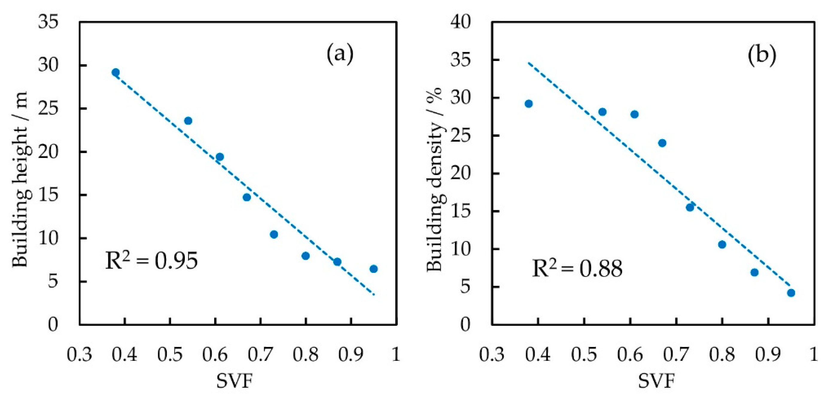
Figure 5.
Urban 3D surface reflectance derived from the urban solar radiative transfer (USRT) model using Landsat 8 data within the study area.
Figure 5.
Urban 3D surface reflectance derived from the urban solar radiative transfer (USRT) model using Landsat 8 data within the study area.
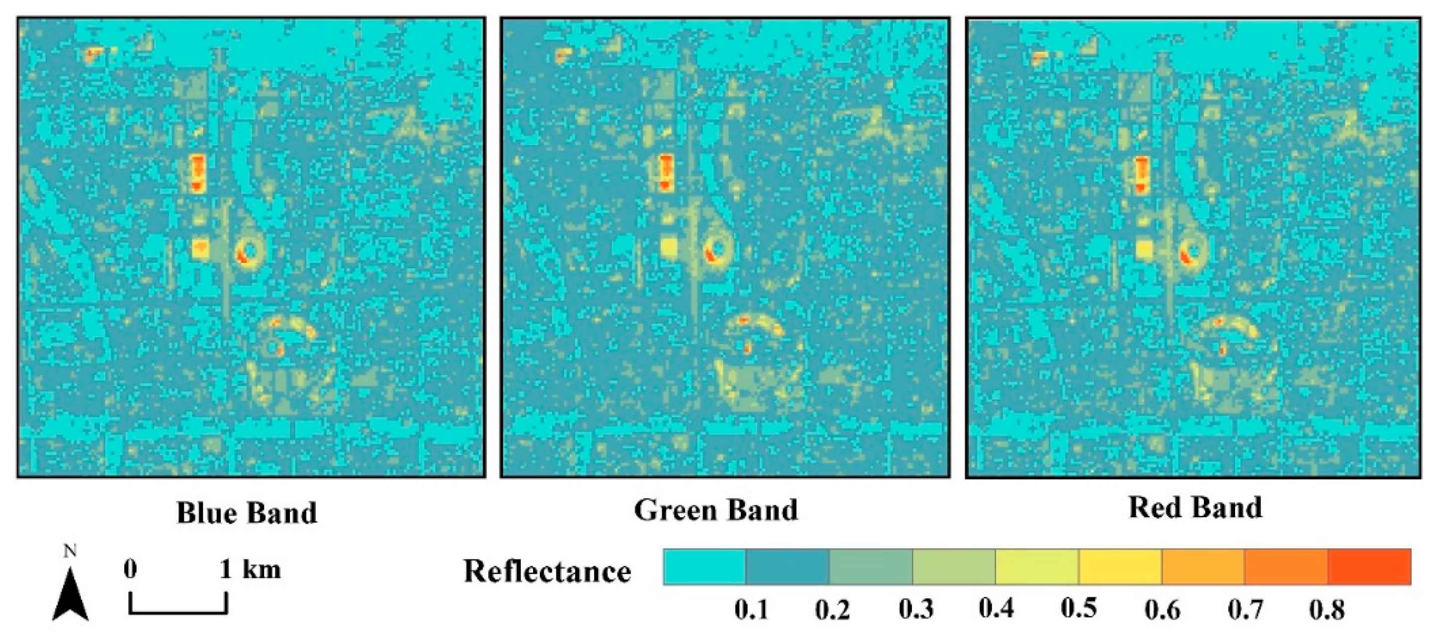
Figure 6.
Schematic diagram of sampling locations in urban and suburban areas. Note: A is in the urban area and B is in the suburban area.
Figure 6.
Schematic diagram of sampling locations in urban and suburban areas. Note: A is in the urban area and B is in the suburban area.

Figure 7.
Urban 3D surface reflectance derived from the USRT model and the flat model: (a) reflectance graph of the blue band; (b) reflectance graph of the green band; (c) reflectance graph of the red band.
Figure 7.
Urban 3D surface reflectance derived from the USRT model and the flat model: (a) reflectance graph of the blue band; (b) reflectance graph of the green band; (c) reflectance graph of the red band.

Figure 8.
Reflectance comparison of the two models with different SVFs. Note: (a) comparison of blue band reflectance from the two models; (b) comparison of green band reflectance from the two models; (c) comparison of red band reflectance from the two models.
Figure 8.
Reflectance comparison of the two models with different SVFs. Note: (a) comparison of blue band reflectance from the two models; (b) comparison of green band reflectance from the two models; (c) comparison of red band reflectance from the two models.

Figure 9.
Reflectance comparison of the two models with different building reflectance. Note: (a) comparison of blue band reflectance from the two models; (b) comparison of green band reflectance from the two models; (c) comparison of red band reflectance from the two models.
Figure 9.
Reflectance comparison of the two models with different building reflectance. Note: (a) comparison of blue band reflectance from the two models; (b) comparison of green band reflectance from the two models; (c) comparison of red band reflectance from the two models.


Table 1.
The simulation results of solar radiative and atmospheric parameters obtaining from the 6S model.
Table 1.
The simulation results of solar radiative and atmospheric parameters obtaining from the 6S model.
| Band | |||||
|---|---|---|---|---|---|
| Blue (0.450–0.515 μm) | 1908.283 | 44.460 | 0.472 | 0.213 | 0.709 |
| Green (0.525–0.600 μm) | 1787.567 | 24.983 | 0.570 | 0.184 | 0.752 |
| Red (0.630–0.680 μm) | 1524.643 | 14.101 | 0.650 | 0.152 | 0.801 |
Table 2.
Average reflectance in blue, green and red band under different SVFs within the study area.
Table 2.
Average reflectance in blue, green and red band under different SVFs within the study area.
| SVF | Blue Band (0.450–0.515 μm) | Green Band (0.525–0.600 μm) | Red Band (0.630–0.680 μm) |
|---|---|---|---|
| [0.24, 0.51) | 0.142 | 0.150 | 0.151 |
| [0.51, 0.58) | 0.138 | 0.152 | 0.143 |
| [0.58, 0.64) | 0.133 | 0.151 | 0.142 |
| [0.64, 0.70) | 0.131 | 0.143 | 0.143 |
| [0.70, 0.76) | 0.120 | 0.139 | 0.130 |
| [0.76, 0.83) | 0.124 | 0.142 | 0.131 |
| [0.83, 0.90) | 0.132 | 0.153 | 0.142 |
| [0.90, 0.99] | 0.151 | 0.170 | 0.162 |
Table 3.
Reflectance comparison of pure grassland pixels derived from the two models in the urban and suburban area.
Table 3.
Reflectance comparison of pure grassland pixels derived from the two models in the urban and suburban area.
| Band | USRT Model | Flat Model | Flat Model |
|---|---|---|---|
| Urban Area | Urban Area | Suburban Area | |
| Blue (0.450–0.515 μm) | 0.074 | 0.073 | 0.076 |
| Green (0.525–0.600 μm) | 0.116 | 0.110 | 0.118 |
| Red (0.630–0.680 μm) | 0.071 | 0.068 | 0.076 |
Publisher’s Note: MDPI stays neutral with regard to jurisdictional claims in published maps and institutional affiliations. |
© 2020 by the authors. Licensee MDPI, Basel, Switzerland. This article is an open access article distributed under the terms and conditions of the Creative Commons Attribution (CC BY) license (http://creativecommons.org/licenses/by/4.0/).
Share and Cite
MDPI and ACS Style
Hu, D.; Liu, M.; Di, Y.; Yu, C.; Wang, Y. USRT: A Solar Radiative Transfer Model Dedicated to Estimating Urban 3D Surface Reflectance. Urban Sci. 2020, 4, 66. https://doi.org/10.3390/urbansci4040066
AMA Style
Hu D, Liu M, Di Y, Yu C, Wang Y. USRT: A Solar Radiative Transfer Model Dedicated to Estimating Urban 3D Surface Reflectance. Urban Science. 2020; 4(4):66. https://doi.org/10.3390/urbansci4040066
Chicago/Turabian StyleHu, Deyong, Manqing Liu, Yufei Di, Chen Yu, and Yichen Wang. 2020. "USRT: A Solar Radiative Transfer Model Dedicated to Estimating Urban 3D Surface Reflectance" Urban Science 4, no. 4: 66. https://doi.org/10.3390/urbansci4040066