Path and Control Planning for Autonomous Vehicles in Restricted Space and Low Speed


Department of Civil Engineering, Ryerson University, 350 Victoria Street, Toronto, ON M5B2K3, Canada
*
Author to whom correspondence should be addressed.
†
These authors contributed equally to this work.
Infrastructures 2020, 5(5), 42; https://doi.org/10.3390/infrastructures5050042
Submission received: 3 April 2020
/
Revised: 3 May 2020
/
Accepted: 4 May 2020
/
Published: 12 May 2020
(This article belongs to the Special Issue Smart Mobility)
Abstract
:This paper presents models of path and control planning for the parking, docking, and movement of autonomous vehicles at low speeds, considering space constraints. Given the low speed of motion, and in order to test and approve the proposed algorithms, vehicle kinematic models are used. Recent works on the development of parking algorithms for autonomous vehicles are reviewed. Bicycle kinematic models for vehicle motion are considered for three basic types of vehicles: passenger car, long wheelbase truck, and articulated vehicles with and without steered semitrailer axes. Mathematical descriptions of systems of differential equations in matrix form and expressions for determining the linearization elements of nonlinear motion equations that increase the speed of finding the optimal solution are presented. Options are proposed for describing the interaction of vehicle overall dimensions with the space boundaries, within which a maneuver should be performed. An original algorithm that considers numerous constraints is developed for determining vehicle permissible positions within the closed boundaries of the parking area, which are directly used in the iterative process of searching for the optimal plan solution using nonlinear model predictive control (NMPC). The process of using NMPC to find the best trajectories and control laws while moving in a semi-limited space of constant curvature (turnabouts, roundabouts) are described. Simulation tests were used to validate the proposed models for both constrained and unconstrained conditions and the output (state-space) and control parameters’ dependencies are shown. The proposed models represent an initial effort to model the movement of autonomous vehicles for parking and have the potential for other highway applications.
1. Introduction
Automated parking within the framework of the general task of autonomous vehicles aims to eliminate the influence of human factors, improving the quality and accuracy of control, and reducing the time and quantity of maneuvers by optimizing vehicle path in restricted parking zones [1,2,3]. The advantages of autonomous parking are not only eliminating routine driver actions, often requiring increased attention and responsibility, but also achieving significant economic benefits, especially for closed areas. The automation of vehicle parking allows one to reduce the lateral distances between parking spaces since there is no more need for opening car doors exactly on a parking spot (a car moves to a parking place autonomously without passengers). A narrow space contributes not only to an increase in parking places but also to a reduction in the unit cost for a parking spot during the construction of parking lots in buildings. The latter is especially relevant due to the promising technologies of vehicle to anything technology, which provides communication between a vehicle and a building through data exchange to find an unoccupied place, to generate the route, and to retain support while moving to a destination. For large-sized trucks, the exceptional importance lies in predicting stable and safe passing on road curved sections, forecasting precise control for docking, followed by discharging and minimizing total control in the case of multiple parameters.
Numerous approaches that consider different control strategies, sensory means, and prediction algorithms have been developed regarding automated parking. Those approaches demonstrate certain similarity in parking modeling. The study by Pérez-Morales et al. [4] is dedicated to perpendicular automated parking with a sensor-based control and weighted control scheme, positioning itself as one of the first attempts in this area. The research included real experiments using the Velodyne VLP-16 compact Lidar, and one part of the study was devoted to the data extraction with followed by determining the loose parking space. The two control methods were considered for kinematic vehicle model: geometric path planning and sensor-based control with evaluating the weighting factors. Despite the fact of using a Lidar and real-world data, some results were unclear, showing the duration of quite simple maneuver about 40 s and the use of steered wheels’ turning without vehicle motion. There was also a pretty big difference between the planned speed and the actual one according to the experiment. Lee et al. [2] proposed using the extended Kalman filter (EKF) with simultaneous localization and mapping (SLAM) algorithm and occupancy grid mapping method for the automated backward perpendicular parking. The authors assert this approach may increase the accuracy for estimating the radar positioning to form a grid map. An algorithm reducing the computational complexity by thresholding the landmark recognition and adaptive changing the state vector length is considered. The scattering extraction using the orthogonal matching pursuit from electric field data is utilized for making realistic simulation of car model’s radar measurements. The authors remark the real-time efficiency of the proposed algorithm improvements.
The study by Lee et al. [1] considers automated parking algorithms for self-driving cars equipped with a lidar such as HDL-32E. Based on 3D point cloud extraction, a parking zone is proposed to be preprocessed for defining the minimum parking space. The path prognosis is based on vehicle dynamics and collision constraints. The fuzzy-logic controller is proposed to be used for controlling the brakes and throttle to sustain stable vehicle speed. The test results obtained by engaging a self-driving car showed the feasibility and efficiency of proposed system for parallel and perpendicular variants of parking. Luca et al. [5] investigated the environment mapping for the case of robotic car parking. The laser scanner SICK LD1000 and ultrasonic sensors perform reliable data for map generation. Implementing evolutive algorithms, the data are being converted into lines denoting the edges of surrounding objects to simplify the parking zone environment. Due to the map’s dynamic evolution while vehicle moving, the data are being checked on merging and fitting by applying a shape correlation, followed by correction. The Embedded Matlab/Simulink Software and the PC104 system are used for testing the navigation and path determination in real-time.
The study by Zhou et al. [6] distinguishes the problem of parking spots’ detection reliability in semi-filled parking lots. The parking zone is supposed to be estimated using onboard laser scanner. The proposed approach aims identifying vehicle bumpers using a supervised learning technique. The classifier is to be trained for recognizing data segments as car bumpers. The developed algorithm creates a topological graph interpreting the parking space to be analyzed. The authors state the algorithm performance has been confirmed by a series of experimental tests. Heinen et al. [7] described a system for implementing the intelligent control for autonomous vehicles. The developed system allegedly can drive a vehicle providing a robust control for parallel automated parking. The sonar sensors are being read for processing the data by a neural network giving steering and accelerating signals. The authors state the proposed controller is perfectly working to park a vehicle in different situations.
Kiss and Tevesz [8] presented a combined approximate method for solving the path planning problem in narrow environments. The approach consists of a global planner that generates a preliminary path consisting of straight and turning-in-place primitives and a local planner that is used to make the preliminary path feasible to car-like vehicles. Lin and Zhu [3] developed a path planner based on a novel four-phase algorithm. By using some switching control laws to drive two virtual cars to a target line, the forward and reverse paths were obtained. Then, the two paths are connected along the target line. The proposed path planning algorithm was fast, highly autonomous, sufficiently general, and could be used in tight environments. Wang et al. [9] proposed a two-stage rapid random-tree (RRT) algorithm to improve computational efficiency. First, the proposed algorithm performs space exploration and establishes prior knowledge represented as waypoints, using cheap computation. Second, a waypoint guided RRT algorithm, with a sampling scheme biased by the waypoints, constructs a kinematic tree connecting the initial and goal configurations. Other researchers also made substantial contributions to the development of parking algorithms. Several ideas considering parking control can be found in such articles as Ballinas et al. [10], Petrov and Nashshibi [11], Gupta et al. [12], Tazaki at al. [13], and Suhr and Jung [14]. Some numerical methods implemented in this paper, such as nonlinear model predictive control (NMPC), have been used in other applications [15,16].
Most of the preceding studies are devoted to the identification of parking zone space and the use of geometric, fuzzy, neural, and other algorithms for predicting vehicle parking path. Many of the studies were accompanied by experiments based on small-scale models or real vehicles. However, most often, for completing a maneuver, the vehicle initial position is pre-set. Thus, clearly there is a lack of research in this field related to vehicle path and control optimization from any current position in restricted space. The purpose of this paper is to develop and test algorithms for parking and docking, based on kinematic vehicle models and nonlinear optimization within limited and unlimited spaces. Composing the unique technique for developing the nonlinear constraints of restricted parking was the main task for applying NMPC in this research.
The next section presents the modelling of autonomous motions of single and articulated vehicles. The following section presents the proposed optimization model, including the basic model and operational, and physical constraints. The implementation of the optimization model is then illustrated using simulation, followed by the conclusions.
2. Kinematic Models of Autonomous Motion
Kinematic vehicle models (Figure 1) are used in this study instead of dynamic models. Kinematic models assume that no slip occurs between the wheels and the road. This assumption is accurate for vehicles moving at low speeds, which is the case for the parking cases developed in this paper. In addition, although dynamic models are generally more accurate, they involve many degrees of freedom that make the model more complex.
2.1. Single Vehicle
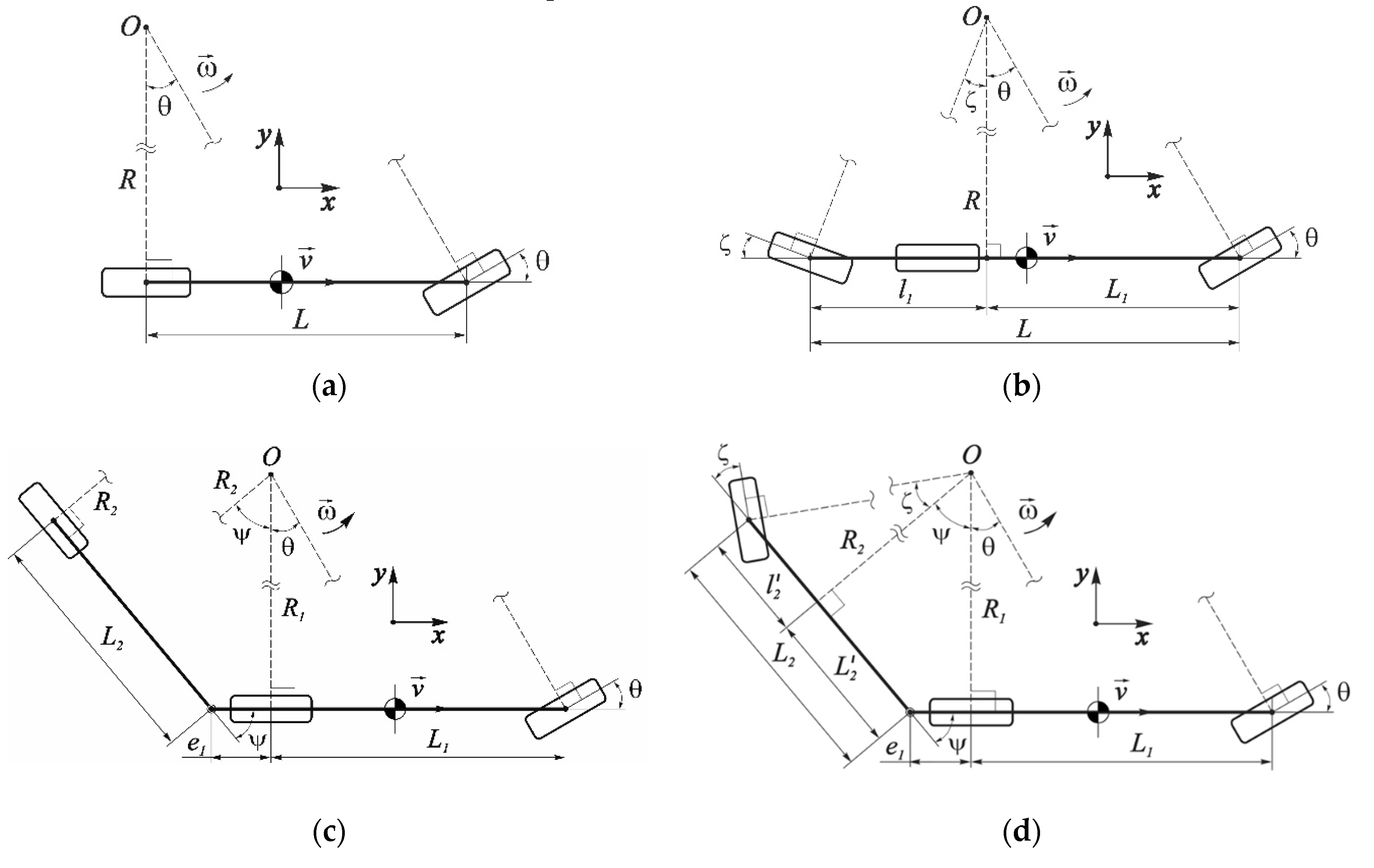
The motion of a single vehicle can be represented as a superposition of elementary rotations around the instantaneous center of velocities. In this case, the vectors of wheels’ translational speeds will be strictly placed in the planes of their rotation. The minimum turning radius for a passenger car model (Figure 1a) passes through the rotational axis of rear wheels and its place is fixed. Thus, the position of the center O is determined only by turning the front steered wheel. This, in turn, affects the excessive sensitivity of the angular velocity ω to the turning angle of the steered wheel and vehicle’s speed. In the case of an additional controlled axis (Figure 1b), the center O is obtained by crossing the perpendiculars to the steered wheels, the ratio of which angles may be different, and therefore the position of minimum turning radius R is not fixed and constantly changes the projection point on the vehicle longitudinal axis. In this regard, the maximum longitudinal base L is constantly divided into variable components L1 and l1.
2.1.1. Passenger Car
In the kinematic bicycle model of a biaxial vehicle, it is assumed that the center of rotation is formed by the intersection of the perpendiculars drawn to the planes of the wheels’ rotation (Figure 1a). In this case, the angular velocity of rotation relative to the instantaneous center of velocities O:
The minimum turning radius R can be determined using the right triangle with the vertex O from the ratio of the steering wheel’s rotation angle θ:
when
The following are model state parameters qi: x denotes vehicle longitudinal displacement, y denotes vehicle lateral displacement, φ denotes vehicle yaw angle, θ denotes vehicle’s front axle steering angle, and v denotes ego vehicle velocity. The derivatives are: vx denotes ego vehicle longitudinal velocity along global x-coordinate, vy denotes ego vehicle lateral velocity along global y-coordinate, and ωφ denotes ego vehicle yaw rate. The control parameters ui are: ωθ denotes vehicle’s front axle steering rate and a denotes ego vehicle longitudinal acceleration. Thus, the control parameters are the longitudinal acceleration and the angular velocity of the steered wheel rotation. Additionally, the input vector of model parameters is p (p = L), where L is the vehicle wheelbase. Then, in vector form,
Reduce the nonlinear function f(q,u,p) to a more convenient form, separating states and controls:
where
Thus,
or
To speed up the search for the optimal solution, as well as for the possibility of using adaptive MPC, consider the linearization of Equation (7), through the expansion in a Taylor series with the first linear terms in the vicinity of point 0. Then, in vector form
where
Obtain,
where
Then, the linearized equation in increments is given by
The matrix A is the Jacobian, which is given by
Substituting Equation (3) into Equation (14) yields
2.1.2. Long Truck with Steered Rear Axle
Unlike the kinematic bicycle model of a biaxial vehicle, it is assumed that in the case of an auxiliary rear steered axle, the perpendicular dropped from the center O to the vehicle’s longitudinal axis and containing the minimum turning radius is floating relative to an intersection point and depends on the ratio of rotation angles of the front and rear axles’ steered wheels (Figure 1b). The angular velocity of rotation relative to the instantaneous center O is determined to be similar to Equation (1). The minimum turning radius R can be determined in two ways, via right angle triangles with a vertex O. From the ratio of the steering angle θ of the front steered wheel:
From the ratio of the steering angle ζ of the rear steered wheel:
Then
Given that the coordinate l1 is negative with respect to the intersection point of radius R, then
Thus,
The expression for the angular velocity is written as
Based on the described and established parameters in Equation (4) for a passenger car, one state ζ (vehicle’s rear axle steering angle) and one control parameter ωζ (vehicle’s rear axle steering rate) should be included to develop the state-space vector for a long single truck:
According to Equation (5),
Thus,
To obtain the Jacobian, denote,
Then, the matrix A (6×6) has the following nonzero elements:
The matrix B remains unchanged.
2.2. Articulated Vehicles
In the case of a conventional articulated vehicle (CAV), by an analogy described in the previous paragraph, two links are being considered whose minimum radii R1 and R2 are crossing in the center of O. Moreover, in the same way, the radius R2 passes through the semitrailer’s conditional middle axle (if 2 axles, then between them). The coupling point is shifted relative to the tractor’s rear axle on the offset e1. Since ψ is the articulation angle, R1 and R2 will also be located at the angle ψ to each other.
While controlling the semitrailer axles, as in the case of a long-base single lorry, the position of the floating point of intersection of the radius R2 and the longitudinal axis of the semitrailer is determined by dividing the base L2 onto L’2 and l’2.
2.2.1. Conventional Tractor-Semitrailer Vehicle
Consider the kinematic bicycle model of a tractor-semitrailer vehicle (TSV). The rotation center is assumed to be formed by the intersection of perpendiculars drawn to the rotational planes of the wheels (Figure 1c). In this case, the angular velocity of the tractor’s rotation relative to the instantaneous center of velocities O will be ω1, and the angular velocity of the semitrailer ω2:
The following are model state parameters qi: x denotes tractor longitudinal displacement, y denotes tractor lateral displacement, φ denotes tractor yaw angle, ψ denotes vehicle articulation angle, θ denotes vehicle’s front axle steering angle, and v denotes tractor velocity. The derivatives are: vx denotes tractor longitudinal velocity along global x-coordinate, vy denotes tractor lateral velocity along global y-coordinate, ωφ denotes tractor yaw rate, and ωψ denotes vehicle articulation rate. The control parameters ui are: ωθ denotes tractor’s front axle steering rate and a denotes tractor longitudinal acceleration. Thus, the control parameters are the longitudinal acceleration and the angular velocity of the front axle’s steered wheel. The parameters p are: L1 denotes tractor wheelbase, e1 denotes fifth wheel offset relative to the tractor’s rear axle (positive if within wheelbase, negative if shifted behind the rear axle), and L2 denotes semitrailer wheelbase, which is the distance from the coupling center (kingpin) to the conditional middle axle. Considering that ψ = φ1 – φ2, dψ/dt = ω1 – ω2, then in vector form,
The angular velocity of the leading unit (tractor) is determined to be similar to Equation (3), replacing L with L1. The semitrailer position could be written as
Then,
As a result, similarly to Equations (23) and (24),
To obtain the Jacobian, similar to Equations (9)–(14), the linearization of Equation (31) is first obtained by letting
Then, the matrix A (6×6) has the following nonzero elements:
The matrix B remains unchanged.
2.2.2. Tractor-Semitrailer Vehicle with Semitrailer’s Steered Axles
The case of the tractor-semitrailer vehicle with semitrailer’s steered axles (TSV-SSA) is similar to the previous case of TSV, except that two parameters are added: the state parameter ζ - (semitrailer’s middle axle steering angle) and control parameter ωζ (semitrailer’s middle axle steering rate), as shown in Figure 1d. Considering Equation (28), The state-space components are given by
The radius R2 may be determined from two conditions, considering Equation (29) and the case of a long single truck:
Then
Considering the coordinate l’2 is negative relative to a cross point of radius R2:
Thus,
The expression for angular velocity ω2 can be derived as:
As a result, similar to Equations (23) and (24),
To obtain the Jacobian, similar to Equations (9)–(14), the linearization of Equation (40) is first obtained by letting,
Then, the matrix A (7×7) has the following nonzero elements:
The matrix B remains unchanged.
3. Optimization Model
3.1. Basic Model
In the general case, for a continuous system, the search condition for optimal control over a finite time interval [t0, tf] can be written as:
Subject to
The function Equation (43) can be represented in discrete form as
where qi denotes vector of state-space parameters at the ith prediction horizon step, Wq, Wu, WΔu denote the matrices of weighting factors, ui denotes control signals at the ith prediction horizon step, zp = (uT0, uTi+1, ··· uTp-1, εp) denotes solution, ε denotes scalar dimensionless slack variable used for constraint softening, ρε denotes constraint violation penalty weight, i denotes current control interval, and p denotes prediction horizon (number of intervals).
The system of constraints is written as:
where qj,min(i), qj,max(i) denote the minimum and maximum values of jth output at the ith prediction horizon step, respectively, uj,min(i), uj,max(i) denote the minimum and maximum values of jth input at the ith prediction horizon step, respectively, Δuj,min(i), Δuj,max(i) denote the minimum and maximum values of jth input rate at the ith prediction horizon step, respectively, h(q)j,min(i), h(q)j,max(i) denote the minimum and maximum values of jth output’s hard constraints at the ith prediction horizon step, respectively, h(u)j,min(i), h(u)j,max(i) denote the minimum and maximum values of jth input’s hard constraints at the ith prediction horizon step, respectively, h(∆u)j,min(i), h(∆u)j,max(i) denote the minimum and maximum values of jth input rates’ hard constraints at the ith prediction horizon step, respectively, nq denotes the number of output parameters, nu denotes number of input parameters, and nΔu denotes the number of input rate parameters.
3.2. Operational and Physical Constraints
3.2.1. Case 1: Vehicle Yaw Rate
As noted, a clear drawback of the kinematic models’ operation at low speeds is the fact that for obtaining the vehicle’s yaw rate ω, the product of the longitudinal speed v and the steering angle θ function is used. This may lead to the case when, if insufficient longitudinal speed, the angular speed is compensated by the intensive changing the turning velocity of steered wheels. This is quite stable from a mathematical point of view but does not correspond to the real nature of the vehicle movement. In turn, it is impossible to directly impose restrictions on the angular rotation velocity in a region of low translational speeds. In this regard, it is assumed that the best solution is to limit the product between the longitudinal speed v and the turning angular velocity of steered wheels ωθ:
where fcr denotes the factor’s critical value.
In this case, at high speeds, the steered wheels’ abrupt turns are absent, and at low values of the vehicle’s longitudinal speed, the wheels’ control turning velocities are limited, which normalizes the nature of the vehicle model movement, especially if the vehicle’s longitudinal speed is close to zero while changing the movement direction.
3.2.2. Case 2: Parking in Restricted Space
Consider the scheme in Figure 2a illustrating a general approach of determining the permissible boundaries between an enclosed space and a passenger car safety contour. In this article, the question of the boundary contour obtaining is omitted but, note, it may be identified by using the SLAM and sensor fusion technologies. As a car moves in an area of potential parking, the surrounding space is scanned by in-vehicle sensors, according to measurements of which a parking loose space shape may be evaluated relative to the vehicle local coordinate system. At the initial position prior to predicting the maneuver, the part of the space that is supposed to be used may be limited by appending the virtual boundaries, which will focus the search for state-space and reduce the optimization time.
Suppose that a car is pre-oriented relative to the desirable final position. Then, a closed perimeter may be virtually represented by a discrete grid with a necessary step along the border (Figure 2a). Note, it is more expedient that the grid density be variable according to space priority, concentrating near the destination. Each node Si of the local space boundaries may be tied by a virtual connection with the vehicle body’s conditional geometric center C, in such a way that a segment CSi by means of a safety contour’s control point Bi is being divided into two components: CBi (associated with the vehicle orientation relative to the initial position) and SiBi (which according to the conditions of maneuver’s safety and accuracy, should always remain positive). Thus, for each i at each predicted moment tk, the following condition must be satisfied:
However, the use of all SiBi values in the nonlinear optimization algorithm is optional, since most of them will certainly be greater than zero, and at each iteration, the SiBi combinations will be different. Therefore, within one iteration of the optimization search, it can be requested that only the minimum SiBi value does not exceed zero. That is,
Now, consider the actual SiBi calculations. The main goal is to determine CBi, since the vehicle contour changes its orientation relative to the initial one (Figure 2c,d). Even though CSi segments converging in the center C (Figure 2c) do not ensure the perpendicularity to the vehicle’s safety contour, this drawback, however, may be compensated by increasing the grid density, considering that point that any violation of vehicle’s safety contour is fully sufficient for determining the constraints. Moreover, as approaching the most distinctive ledges of the parking zone perimeter, the CSi distances are reduced and their directions become more and more similar to perpendiculars passing through the safety contour.
The virtual security points of vehicle contour can also be set in discrete form. Any form that outlines the overall vehicle dimensions along its perimeter with some safety margin may be represented in polar coordinates (Figure 2b) in such a way that, for any n, an unambiguous determination in the vehicle’s initial position is established between an angle αn0 and a point Pn0. In this case, the internal points within the nodes can be determined using an interpolation (linear or spline, depending on priorities).
Because of plane representation (bird’s-eye view) of the vehicle movement in a parking lot, the safe contour’s motion relative to the absolute XOY system can be divided into translational and rotational (Figure 2c,d).
In the case of translational motion (Figure 2c), the point Si of the parking space perimeter relative to the car contour’s initial position x0C0y0 forms the point Bi0 on the angle βi0, and in the state xkCkyk the point migrates to the position Bik on the angle βik. If one considers this situation from the car’s local coordinate system xCy, all the segments CSi will rotate relative to the safe contour. Therefore, using the interpolation approach in accordance with the prepared basis (Figure 2b), it is possible to recalculate the points’ Bik positions by the known angles βik, which, in turn, are obtained based on the known coordinates of Si and Ck.
In the case of the car contour’s rotational movement (Figure 2d), the segment C0Si is identical to the segment CkSi, but due to the vehicle’s turn to an angle φk, the new angular position βik will be defined as:
Considering that the state-space parameters q are iterative during the optimization process, their current values are known, and thus, the segments’ CkSi current angular directions relative to the local coordinate system x0C0y0 can be determined by the superposition of the parking boundary’s relative displacement and rotation. Thus, at each iterative step k, the Si nodes’ coordinates due to translation in the vehicle’s coordinate system x0C0y0 are:
where xSk, ySk denote vectors of zone contour nodes’ coordinates in the coordinate system x0C0y0, xS0, yS0 denote vectors of zone contour nodes’ coordinates in the global coordinate system XOY, and xCk, yCk denote displacements of the safe contour’s center Ck in the global coordinate system XOY. The distances rSik from the nodes Sik to the center Ck and the angles βik at time interval k in the coordinate system xkCkyk:
Then, knowing the new angles βik and the base angles αn0 with the corresponding xn0, yn0, the coordinates of points Bik can be obtained:
where xBk, yBk denote vectors of safety contour points’ coordinates at time step k, fx, fy denote parametric interpolation functions for xk and yk coordinates, respectively, α0 denotes vector of segments’ C0Si angles at initial state, x0, y0 denote vectors of contour control points’ coordinates at initial state, and βk denotes vector of current segments’ CkSi angles, Equation (47).
The distances from center Ck to points Bik in the coordinate system x0C0y0 at time interval k are:
Then, the condition for the car safety contour’s violation absence at time interval k is given by
The last condition is added to the vector of inequality constrictions of optimization conditions.
3.2.3. Case 3: Circular Motion
The idea of constraints with constant curvature is that the trajectories of the vehicle contour’s n given points must lay within the considered boundaries. Each such a Bn point (like Figure 2b) is distanced by a radius rBn from the contour’s center and compose an angle αBn with the vehicle local coordinate system’s longitudinal axis. Thus, in the global coordinate system XOY, the Bn points’ coordinates XBnk, YBnk for kth prediction horizon step yield:
Correspondingly, the radii of controlling points in the global coordinate system XOY:
Then, the condition of nonlinear restrictions for each kth prediction horizon step is:
where Rin and Rout denote the inner and outer radii of a roundabout, respectively.
4. Simulation
There are various schemes of the model predictive control method that provide optimal solutions for guaranteeing the robustness under conditions of complex restrictions; see Garcia et al. [17] and Lu and Arkun [18]. Basically, for each horizon interval, the scheme solves an optimization problem with respect to the constraints. The NMPC provided by MATLAB software [19] was used for predicting vehicle behavior and control on a finite-time interval. To plan optimal trajectories, the NMPC controllers solve an open loop constrained nonlinear optimization problem using the SQP algorithm. For each design vehicle, an NMPC object combining model-based prediction and constrained optimization was created. Accordingly, all vehicle models, equality and inequality constraints are nonlinear. The cost function may not necessarily be a quadratic function, which gives more flexibility in finding an appropriate solution. Restrictions may be imposed on inputs (control), outputs, and states. Three types of design vehicles were simulated: passenger car, long single truck with steered rear axle, and articulated vehicles (conventional AV and AV with steered axle of semitrailer). The restrictions and initial conditions for various types of motions are shown in Table 1 for a passenger car, Table 2 for long single trucks and in Table 3 for articulated vehicles. For simplicity, all the weighting factors of the objective functions were set as equal to 1.
4.1. Simulation of Passenger Car
For a passenger car, the only parameter is the longitudinal wheelbase L which equals 2.8 m. Equations (8)–(15) are used for model prediction. For the parking maneuver (Figure 3, Figure 4a,b), the quadratic linear form of the cost function works well, while optimizing without restrictions when the minimum of a cost function is absolute. Moreover, due to the quadraticity, the results give the smoothest functions of the state parameters, which rarely change their sign within the prediction horizon. However, the imposition of restrictions narrows the area of optimum search and complicates the task, where conditional optimality may also be acceptable. In the case of parking, the priority is not so much the optimality of solution as the maneuver accuracy with the possibility of arbitrarily using the space and directions of movement (forward and backward). In view of the latter, it is proposed that one uses a linear function as the target one that relaxes the search and reduces the time of iterations. The inequality constraints are based on Equation (54).
where eq, eu denote unit vectors of the same dimension as q and u, respectively, Wq, Wu denote weighting factors, and zp denotes solution vector.
For the circular motion (Figure 4b,c), control is a priori the simplest, due to retaining the steering angle θ value of a narrow range. The cost function has the form:
This is subject to an inequality constraint given by Equation (57).
4.2. Simulation of Long Single Truck with Steered Rear Axle
The parameter for this model is the full wheelbase L = L10 + l10, consisting of longitudinal wheelbase L10 = 6.65 m between steering and driving axles and spread axles’ wheelbase l10 = 1.4 m. Equations (24)–(26) are used for model prediction. Consider first the parking maneuver (Figure 5a,b). In the case of perpendicular reverse parking, the following objectives are set for optimizing the maneuver: reducing the use of space, ensuring the smoothness of the control functions, and redistributing the control between the vehicle’s steered axles to provide the minimal total steering control. In particular, the vehicle maneuver is better to be oriented in a way that there are the perpendicular and the parallel phases resembling the letter “L” relative to an unoccupied parking place. In this regard, it is expedient to minimize the use of corresponding x and y coordinates. Then, considering constraints set in Equation (54), the cost function can be derived as a combination:
where Wu denotes the control weighting factor and Wθζ denotes weighting factor of mutual influence between θ and ζ.
In the case of changing position on the spot (Figure 5c,d), the task is complicated with the fact that the initial and final coordinates of the vehicle’s mass center are coincident. To realize the maneuver, the cost function needs to be relaxed by allowing the controller searching for a solution in both positive and negative zones. The linear cost function can be represented by the sum of Cartesian coordinates x and y, Equation (22):
For the circular motion (Figure 6); on the one hand, there is a need for softening the inequality constraints set in Equation (57) within the boundaries of a roundabout’s lane width. On the other hand, it is desirable to ensure the minimum space occupied by the vehicle with the smooth and minimal total steering control. Thus, a combination of linear and non-linear cost function elements may be used:
where Wq = diag(1, 1, 1, 0, 0, 1) denotes the diagonal matrix of states’ weighting factors, eq denotes unit vector of the same dimension as q, eu denotes unit vector of the same dimension as u, Wu denotes control weighting factor, Wθζ denotes weighting factor of mutual influence between θ and ζ.
4.3. Simulation of Articulated Vehicles
According to the designation in Figure 1c,d, the models are characterized by three parameters: L1 = 3.8 m, L2 = 7.57 m, e1 = 0.47 m. Equations (28), (31), (33), (34), (40), and (42) are used for model-based prediction, and all the symbols correspond to those ones in figures.
Consider first docking at unconstrained space (Figure 7). Usually, the loading and unloading of articulated vehicles are carried out from the side of the warehouses’ docks, where there is a lot of space for the maneuvering of long vehicles. In this regard, the spatial restrictions may be omitted. In the case of conventional TSV (Figure 7a,b), considering the space between initial and final positions is not being restricted, a relatively symmetric distribution of coordinates, speed, and control may be satisfactory, which mitigate the search with a linear cost function, avoiding the redundant smoothness. Hence, it may be presented as:
where Wq = diag(1,1,1,1,0,1) denotes diagonal matrix of states’ weighting factors, and other symbols are as previously defined.
In the case of TSV-SSA (Figure 7c,d), the vehicle may occupy as much space as needed for the maneuver. As the vehicle is charged and in order to prevent significant tires’ sideslip, it is undesirable for its links to be folded on a big angle. Meanwhile, there is no strict necessity that the tractor center’s trajectory be highly smoothed. Thus, a linear function of the tractor’s translational and rotational states would be enough. The control must provide smooth motion in general and total steering action should be reduced as well. Consequently, the cost function may be written in a form:
where Wq = diag(1,1,1,0,0,0,0) denotes diagonal matrix of states’ weighting factors, and Wθζ denotes weighting factor of mutual influence between θ and ζ.
For the circular motion, in the case of conventional TSV (Figure 8a,b), the controlling of the vehicle links’ mutual orientation (articulation angle ψ) is possible only by the tractor’s steered wheels. However, according to the tractor movement conditions relative to the center of a roundabout, the wheels’ position θ is determined in a narrow range.
Within the specified lane width H, certain control is feasible, ensuring the minimum possible articulation angle. Then, considering Equation (31), the cost function can be written in the linear-quadratic form:
In the case of TSV-SSA (Figure 8c,d), the idea is that the vehicle should occupy the minimum space at a roundabout, which corresponds to keeping the articulation angle ψ in the region of the smallest possible value for a given circle with the narrowest corridor H. In addition, it is desirable that the control signals be as smoothed as possible, and the total control of tractor’s θ and semitrailer’s ζ wheels is synchronized and minimal as well. Thus, considering Equation (34), the cost functional can be written as:
4.4. Results and Discussion
Based on the optimized paths for the vehicles’ motion plans, the visualizations of predicted trajectories are depicted, as well as graphs of the main output parameters (linear, angular displacements, ego speeds, and steering angles) and control laws (accelerations and steered wheels’ angular speeds). The technique presented in paragraph 4, in general, has shown its effectiveness, allowing one to plan successful maneuvers with various combinations of initial and final conditions on a finite prediction horizon. The obvious advantage of the optimization approach is that the steering angles evolve with a change in vehicle speed, i.e., in fact, there is no wheel turn on the spot. The aim of forecasting the circular motion is to work out the restrictions for any type of curvilinear motion with variable road curvature, for cases of assigning a lane to an articulated vehicle, as well as when narrowing the space allocated to a vehicle. The hard restrictions lead to some fluctuations in solutions. To have smooth gentle output curves, it is necessary to narrow the range of constraints of state parameters within the framework of vehicle kinematic models.
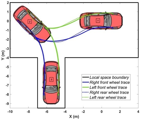
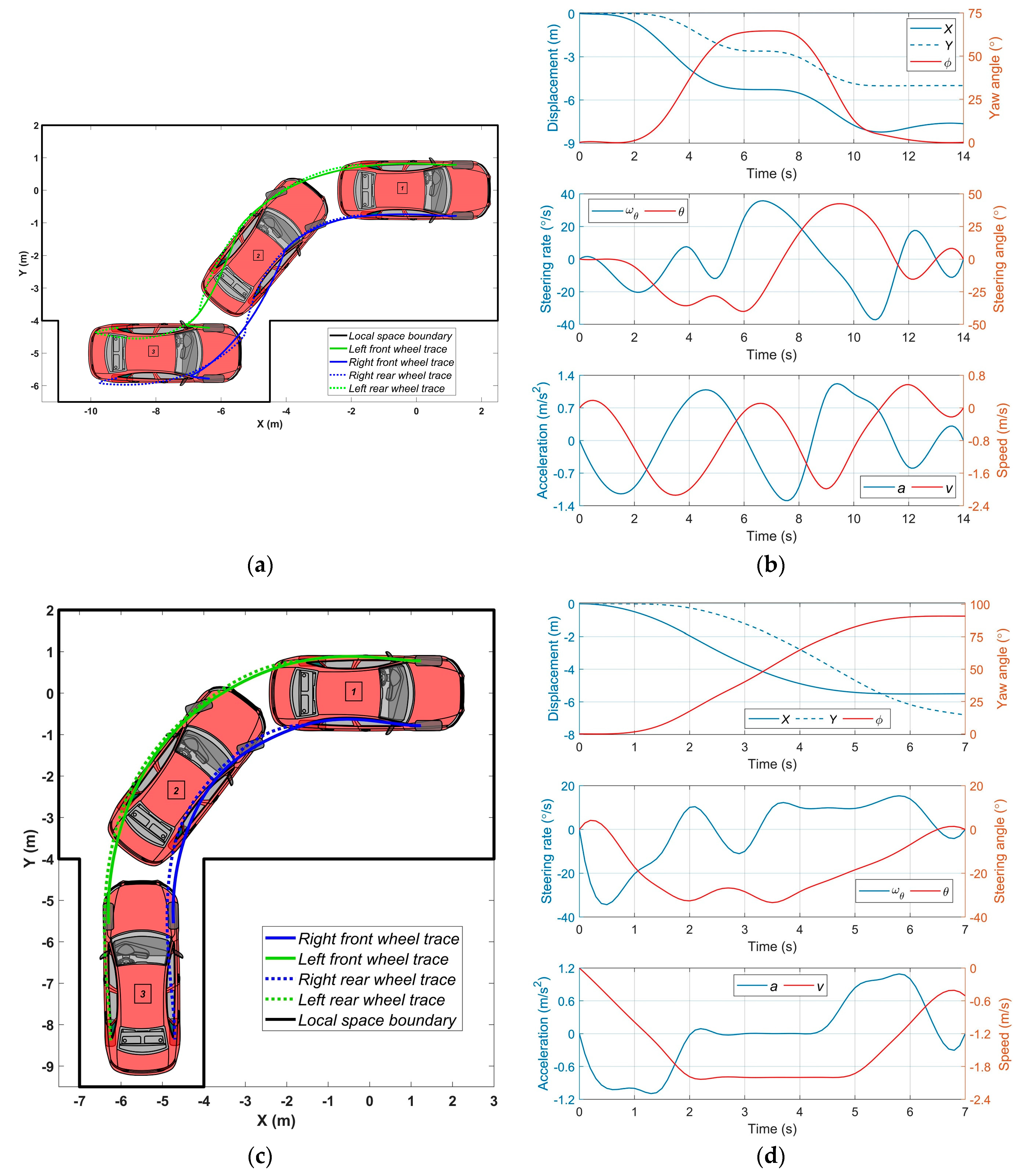
The simulation results for the car parallel reverse parking are presented in Figure 3a,b. The initial conditions are given in Table 1. In this example, the task consists of predicting the maneuver and the control factors for placing a car in a parking spot from the parallel initial position in a finite time. In fact, the car initial position relative to the parking pocket can be specified by an arbitrary initial vector q0, however, it is more expedient to choose a position at which the distance to the destination is minimal and the complexity of the maneuver is quite high. Due to the linear form of the objective function Equation (58) the car speed v (Figure 3b) may change a sign, which corresponds to shifting vehicle direction for better adapting to local space. When approaching a sharp edge of the pocket (Figure 3a) at the sixth second, the speed module value decreases. The graph of the steering angle θ shows an intensive adaptation of the vehicle angular position using the full range of steering angle. Nevertheless, the resulting output parameters of the car angular and linear displacements X, Y, φ show smooth properties (Figure 3b), which in general can characterize the parking process as stable.
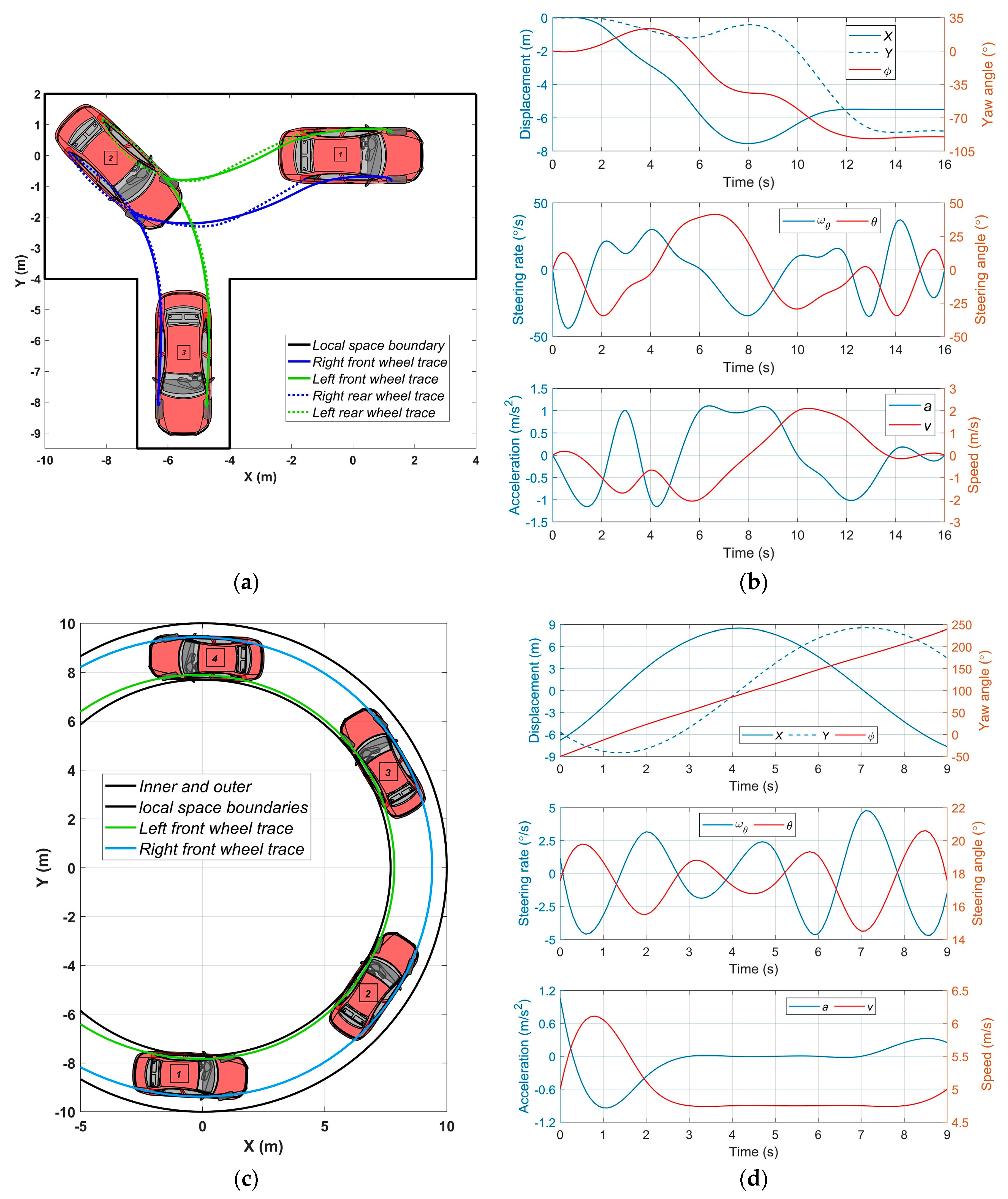
The results for car perpendicular reverse parking are presented in Figure 3c,d. This maneuver is the simplest in terms of control. In some works, the necessary trajectory is determined geometrically by an arc of constant radius. However, this is acceptable if the initial position of the vehicle is determined in the vicinity of an acute angle of the parking pocket. In the case of an arbitrary position, it is important to orient the vehicle in phase 2 as coaxially as possible to the pocket axis when a car may maintain an approximately permanent value of ego velocity v. In this regard, at the initial moment, the steered wheels have a positive angle of rotation θ, which first leads the car’s rear to the outer boundary. It is noteworthy that the rotation angle and speed signals are of a general tendency but not synchronous. The results for car perpendicular forward parking are presented in Figure 4. Such a maneuver is possible with sufficient space outside a parking pocket. It consists of two phases: partial reverse turn (1–2) and forward turning (2–3). The maneuver is quite long, 16 seconds, however, NMPC successfully built the forecast for it. The control parameters a and ω begin and end with zero values; the values of the steering angle θ are used in the full range, which indicates the need for a high degree of maneuverability in the given constraint conditions. It can be noted that the final phase is characterized by almost constant values of the yaw angle and the X coordinate, and the speed v decreases to the utmost, which indicates a stable and safe car movement relative to the destination and the parking spot borders.
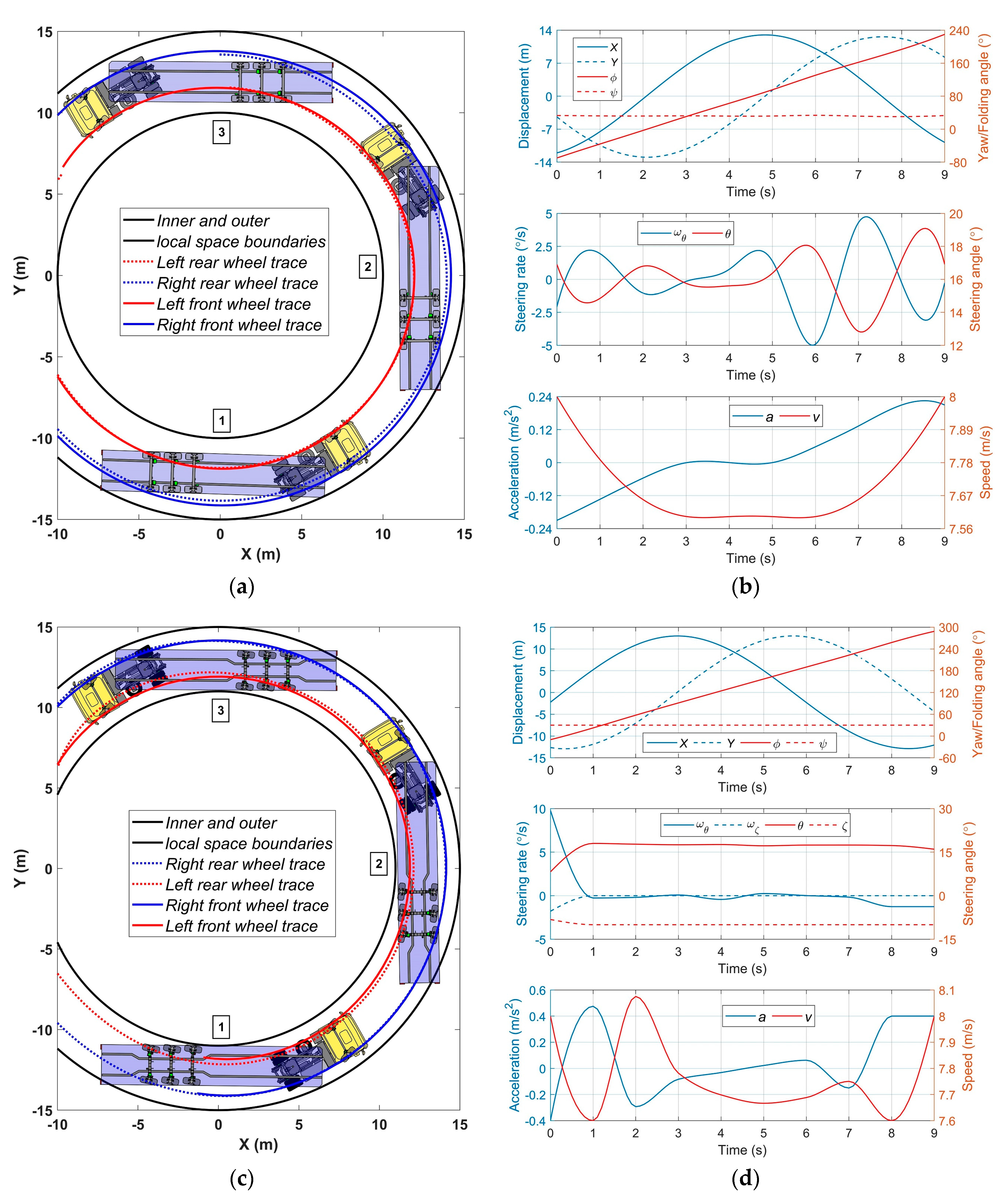
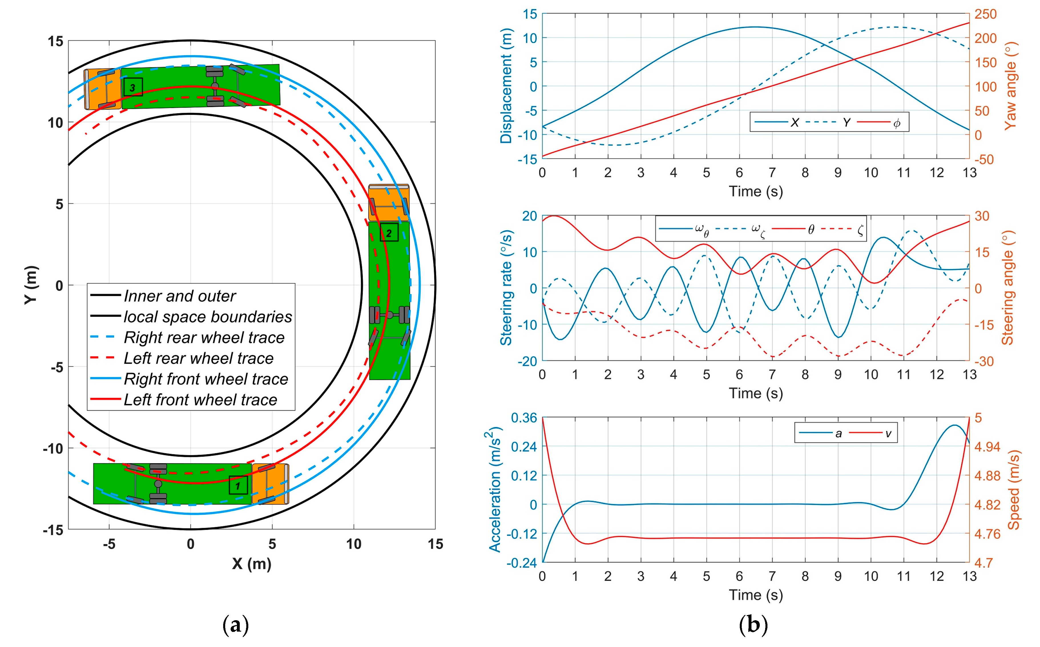
The results for car circular motion are presented in Figure 4c,d. When planning a circular motion, it should be considered that the closer values of vectors of initial and final conditions, especially the coordinates in the restrictions of tight boundaries, the more the solution instability. The space of a road curved section defined by lidar or camera locks up on the prediction horizon. Therefore, the planning makes sense only within the framework of an arc defined by the values of initial and final angular coordinates βC0, βCf in Table 1. In this example, there is no hard restriction on the desired speed value and therefore the speed v varies in the range of 5-6 m/s, with practically zero acceleration a. The average value of the steering angle is kept at the level of 18°, and the fluctuations are stipulated by the deterministic tie with a speed change. Nevertheless, the output characteristic of the yaw angle is almost linear, which demonstrates the stability and constancy of the yaw rate.
The results for truck perpendicular reverse parking are presented in Figure 5a,b. This maneuver is modeled for the case when the same type long wheelbase vehicles are placed in a row and there is a free spot. The use of an auxiliary steered axle allows increasing vehicle maneuverability and ensuring the best control accuracy and space use. The truck has zero initial data in the initial position. The approach of describing the space represented in Figure 2. As can be seen, the output and control parameters are smooth curves, clearly reflecting the maneuver phases. The angular velocities ωθ, ωζ of steering wheels, as well as their turning angles θ and ζ, are in antiphase within a wide range of admissible values.
The results for changing truck position on the spot are presented in Figure 5c,d. The maneuver corresponds to the case of the most limited space if there is a need for changing the truck position. The linear form of the objective function Equation (61) is focused on the minimum use of coordinates, which is enhanced by the simultaneous control of two axles with the maximum ranges of steering angles θ and ζ. First, the vehicle moves backwards from state 1 to state 2, and then forward to the final position 3. The vehicle speed module does not exceed 2 m/s, and the whole process takes about 17 s. The graph of accelerations clearly shows the number of sign changes of longitudinal accelerations, which indicates the nature of the acceleration-deceleration control. As can be seen from the graphs, the initial and final values of linear displacements coincide, and the angular coordinates have a difference of 90 °. The results for truck circular motion are presented in Figure 6. The need for such a maneuver is explained by the emerging need for the accurate prediction of curvilinear motion in conditions of minimal swept path. The output yaw angle demonstrates an almost linear increase. Some fluctuations in the steering rates ωθ, ωζ and the steering angles θ and ζ are explained by the influence of the truck long wheelbase and by the simultaneous control of two axles, which brings an oversteer tendency to the kinematic model. Nevertheless, the output linear displacements X, Y, φ are stable and represented by smooth curves, without any ambiguity in curvature changes.
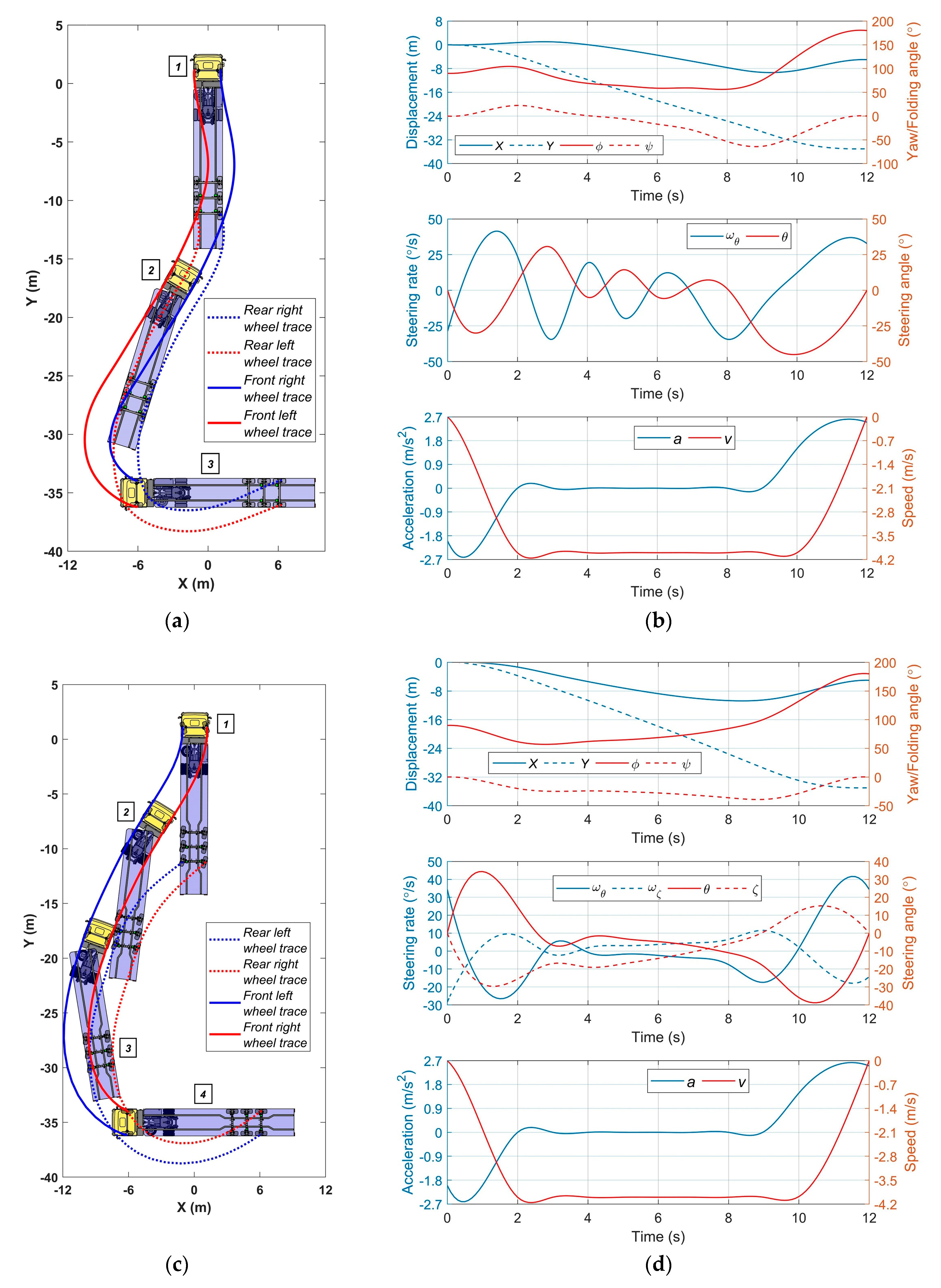
The results for an articulated vehicle docking in an unconstrained space for TSV and TSV-SSA docking are presented in Figure 7. The purpose of the maneuver is to obtain the simplest control while minimizing the use of space and state parameters. However, there are no restrictions on the use of space. The task is to perform a maneuver in reverse with a turn on 90 ° to the place of supposed unloading. As can be seen in Figure 7b,d, the distribution of acceleration and speed over time is almost identical for the TSV and TSV-SSA, however, for the control signals of the steering rates and, as a consequence, the steering angles—there is a significant difference. When using the TSV-SSA, the required control is both more stable and smaller in range due to oversteer. Moreover, TSV-SSA has a much lesser range of articulation angle. The results for articulated vehicle circular motion for TSV and TSV-SSA are presented in Figure 8. The maneuver purpose is to optimize the disposition of an articulated vehicle in conditions of movement along a lane of a roundabout (turnabout) or other arched road sections with a small curvature radius. Since the acceleration a of TSV in Figure 8b is variable, the control signal of the steering rate ωθ fluctuates, however, the average value of steered wheels’ angle is about θ = 16 °, and the output linear and angular displacements X, Y, φ are represented by smooth curves, including a stable folding angle ψ close to a constant value. In the case of TSV-SSA, the situation is tougher. The vehicle is situated in a very narrow corridor to be accommodated. The swept path should be minimal. As seen in Figure 8d, in this case, all the control parameters ωθ, ωζ and the states θ, ζ, and ψ are practically invariable within the prediction horizon.
5. Conclusions
This paper has presented nonlinear kinematic models for vehicle path and control forecasting using an open-loop optimization technique for predicting vehicle behavior in the low-speed range and space-limited areas. The study has proposed a parking algorithm and has evaluated the implementation of NMPC for such objectives, in general, and for the possible use in the closed-loop tracking combined with dynamic vehicle models. In addition, the study has revealed the modeling nuances, advantages, and disadvantages of applying kinematic models. Based on this study, the following comments are offered:
- Based on the positive results in all the simulations, the use of kinematic models’ trajectories for the tracking is quite suitable for low speeds, when the trajectories are supposed to be represented by smooth curves. However, the shape of control signals reflects, to a greater measure, the disadvantages of kinematic models’ indirect control (by acceleration) and to a lesser measure reflects the direct control parameter (throttle position and power).
- The presented original algorithms consider the indirect parameter - the intrusion into a vehicle safety contour (or the excess of a pre-set level by control points) to model the inequality constraints. The proposed idea has shown the adequate accuracy in assessing the inadmissible distances to a vehicle body. The simplicity and versatility can be marked as an advantage of the proposed method, and the fact that it is a part of the optimization process and not just a geometric technique. The proposed technique can also be easily used for simulating the avoidance of moving and stationary obstacles.
- The cost function form significantly affects the forecast, depending on the accepted optimality criteria. The advantage of the specified NMPC is the ability to use any functions, both linear and non-linear, and their combinations. Unlike the lane change at high speeds, where the smoothness is required and quadratic forms are frequently used, the linear functions and quasi-optimal solutions are often quite adequate at low speeds. Thus, it was revealed that the cost function’s linear components work better where changes of vehicle model speed’s signs are expected, and a shorter maneuvering path is needed. Quadratic forms provide more smoothed control and allow better coordination of combined control (the case of several steered axles).
- This project may be considered as a test phase of a comprehensive study of parking/docking algorithms for autonomous vehicles. The results have argued the applicability of kinematic models and the quality of forecast in general. Within the expansion of elaborating the automated parking algorithms, it is planned to include the following issues: mapping the parking space using the SLAM methods, improving the constraint evaluation algorithm to an adaptive level, creating and testing the alternative algorithms for constraints, developing dynamic vehicle models with real-world control parameters, implementing nonlinear and adaptive MPC methods for the tracking task, and combining the parking computing techniques into one automated option for HIL-testing.
Author Contributions
Conceptualization, M.D. and S.M.E.; methodology, M.D.; software, M.D.; validation, J.B.; formal analysis, J.B.; investigation, M.D.; resources, S.M.E.; data curation, J.B.; writing—original draft preparation, M.D., J.B.; writing—review and editing, S.M.E.; visualization, M.D.; supervision, S.M.E.; project administration, S.M.E.; funding acquisition, S.M.E. All authors have read and agreed to the published version of the manuscript.
Funding
This research was financially supported by the Natural Sciences and Engineering Research Council of Canada (NSERC).
Acknowledgments
The authors are grateful to two anonymous reviewers for their thorough and most helpful comments.
Conflicts of Interest
The authors declare no conflict of interest. The funders had no role in the design of the study; in the collection, analyses, or interpretation of data; in the writing of the manuscript, or in the decision to publish the results.
Abbreviations
The following abbreviations are used in this paper:
| AV | Autonomous vehicle |
| CAV | Conventional articulated vehicle |
| EKF | Extended Kalman filter |
| HIL | Hardware-in-the-loop |
| NMPC | Nonlinear model predictive control |
| SLAM | Simultaneous localization and mapping |
| SQP | Sequential quadratic programming |
| TSV | Tractor-semitrailer vehicle |
| TSV-SSA | Tractor- semitrailer vehicle with semitrailer’s steered axles |
References
- Lee, B.; Wei, Y.; Guo, I.Y. Automatic parking of self-driving car based on Lidar. International Archives of the Photogrammetry. Remote Sens. Spat. Inf. Sci. 2017, 42, 241–246. [Google Scholar]
- Lee, H.; Chun, J.; Jeon, K. Autonomous back-in parking based on occupancy grid map and EKF SLAM with W-band radar. In Proceedings of the International Conference on Radar (RADAR), Brisbane, Australia, 27–30 August 2018; pp. 1–4. [Google Scholar]
- Lin, L.; Zhu, J.J. Path planning for autonomous car parking. In Proceedings of the ASME Dynamic Systems and Control Conference, Atlanta, GA, USA, 30 September–October 3 2018; Volume 3. [Google Scholar]
- Pérez-Morales, D.; Domínguez-Quijada, S.; Kermorgant, O.; Martinet, P. Autonomous parking using a sensor-based approach. In Proceedings of the IEEE 19th International Conference on Intelligent Transportation Systems (ITSC), Rio de Janeiro, Brazil, 1–4 November 2016. [Google Scholar]
- Luca, R.; Troester, F.; Gall, R.; Simion, C. Environment mapping for autonomous driving into parking lots. In Proceedings of the IEEE International Conference on Automation, Quality and Testing, Robotics (AQTR), Cluj-Napoca, Romania, 28–30 May 2010; pp. 1–6. [Google Scholar]
- Zhou, J.; Navarro-Serment, L.E.; Hebert, M. Detection of parking spots using 2D range data. In Proceedings of the IEEE International Conference on Intelligent Transportation Systems, Anchorage, AK, USA, 16–19 September 2012; pp. 1280–1287. [Google Scholar]
- Heinen, M.R.; Osorio, F.S.; Heinen, F.J.; Kelber, C. SEVA3D: Using artificial neural networks to autonomous vehicle parking control. In Proceedings of the IEEE International Joint Conference on Neural Network, Vancouver, BC, Canada, 16–21 July 2006; pp. 4704–4711. [Google Scholar]
- Kiss, D.; Tevesz, G. Autonomous path planning for road vehicles in narrow environments: An efficient continuous curvature approach. J. Adv. Transp. Intell. Auton. Transp. Syst. Des. Simul. 2017. [Google Scholar] [CrossRef] [Green Version]
- Wang, Y.; Jha, D.K.; Akemi, Y. A two-stage RRT path planner for automated parking. In Proceedings of the 13th IEEE Conference on Automation Science and Engineering, Xi’anChina, 20–23 August 2017; pp. 496–502. [Google Scholar]
- Ballinas, E.; Montiel, O.; Castillo, O.; Rubio, Y.; Aguilar, L.T. Automatic parallel parking algorithm for a car-like robot using fuzzy PD+1. Control. Eng. Lett. 2018, 26, 447–454. [Google Scholar]
- Petrov, P.; Fawzi, N. Automatic vehicle perpendicular parking design using saturated control. In Proceedings of the IEEE Jordan Conference on Applied Electrical Engineering and Computing Technologies, Amman, Jordan, 3–5 November 2015; pp. 1–6. [Google Scholar]
- Gupta, A.; Rohan, D.; Mohit, A. Autonomous parallel parking system for Ackerman steering four wheelers. In Proceedings of the IEEE International Conference on Computational Intelligence and Computing Research, Coimbatore, India, 28–29 December 2010; pp. 1–6. [Google Scholar]
- Tazaki, Y.; Okuda, H.; Suzuki, T. Parking Trajectory Planning Using Multiresolution State Roadmaps. IEEE Trans. Intell. Veh. 2017, 2, 298–307. [Google Scholar] [CrossRef]
- Suhr, J.K.; Jung, H.G. Automatic parking space detection and tracking for underground and indoor environments. IEEE Trans. Ind. Electron. 2016, 63, 5687–5698. [Google Scholar] [CrossRef]
- Diachuk, M.; Easa, S.M.; Hassein, U.; Shihundu, D. Modeling passing maneuver based on vehicle characteristics for in-vehicle collision warning systems on two-lane highways. Transp. Res. Record 2019, 2673, 165–178. [Google Scholar] [CrossRef]
- Diachuk, M.; Easa, S.M. Guidelines for roundabout circulatory and entry widths based on vehicle dynamics. J. Traffic Transp. Eng. 2018, 5, 361–371. [Google Scholar] [CrossRef]
- Garcia, C.E.; Prett, D.M.; Morari, M. Model predictive control: Theory and practice—A survey. Automatica 1989, 25, 335–348. [Google Scholar] [CrossRef]
- Lu, Y.; Arkun, Y. Quasi-Min-Max MPC algorithms for LPV systems. Automatica 2000, 36, 527–540. [Google Scholar] [CrossRef]
- MathWorks. Available online: www.mathworks.com (accessed on 1 August 2019).
Figure 1.
Kinematics of curvilinear motion for different types of vehicle design: (a) Passenger car; (b) Single truck with steered rear axle; (c) Conventional tractor-semitrailer vehicle (TSV); (d) Tractor- semitrailer vehicle with semitrailer’s steered axles (TSV-SSA).
Figure 1.
Kinematics of curvilinear motion for different types of vehicle design: (a) Passenger car; (b) Single truck with steered rear axle; (c) Conventional tractor-semitrailer vehicle (TSV); (d) Tractor- semitrailer vehicle with semitrailer’s steered axles (TSV-SSA).

Figure 2.
Determining mutual disposition between vehicle safe contour and parking area boundary: (a) Scheme of the general idea; (b) Vehicle’s safe contour control points; (c) Control points due to vehicle translational motion; (d) Control points due to vehicle rotation.
Figure 2.
Determining mutual disposition between vehicle safe contour and parking area boundary: (a) Scheme of the general idea; (b) Vehicle’s safe contour control points; (c) Control points due to vehicle translational motion; (d) Control points due to vehicle rotation.
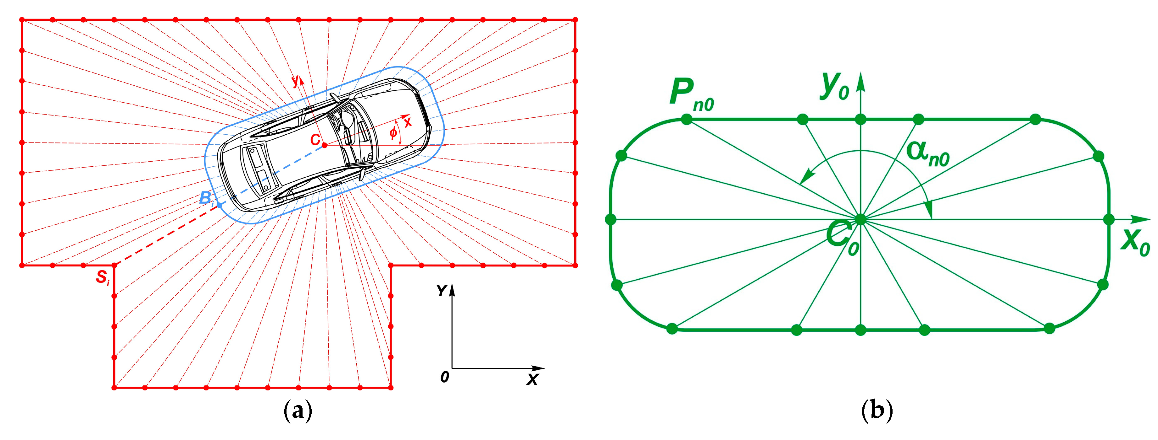
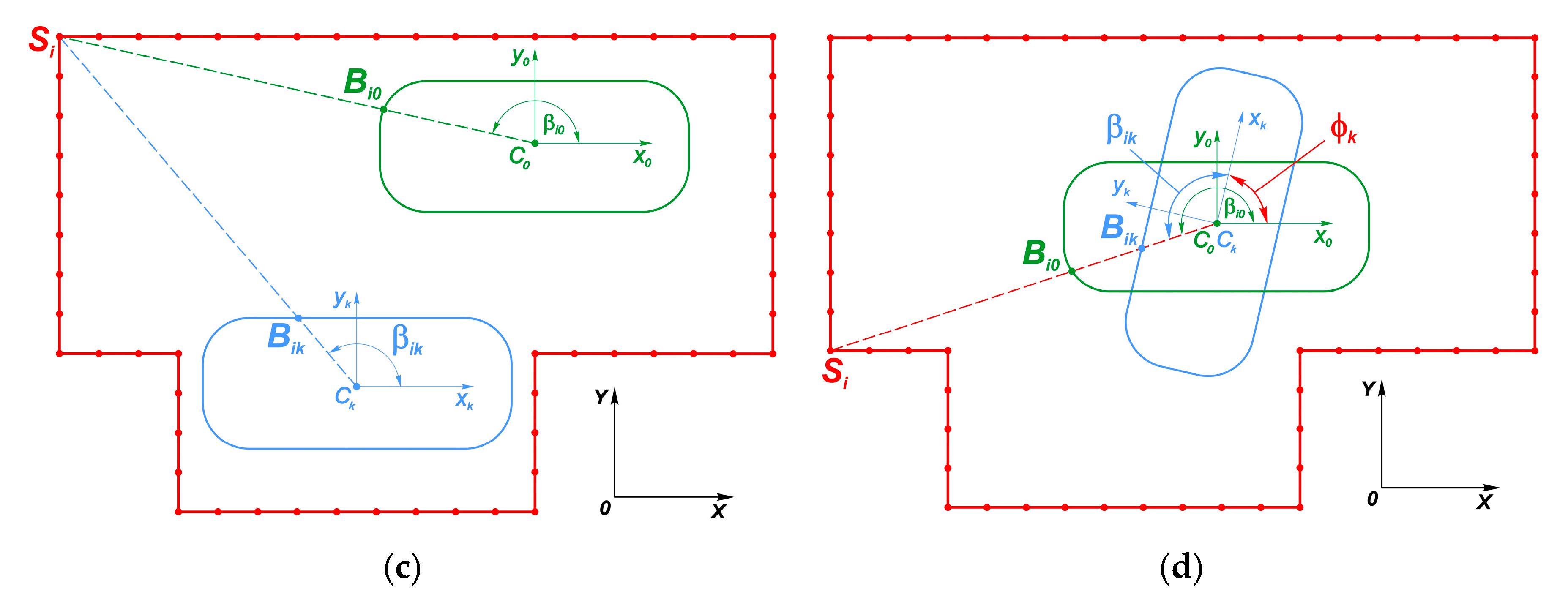
Figure 3.
Simulation results for reverse parking of a passenger car: (a) Position and trajectory (parallel reverse); (b) Basic parameters (parallel reverse); (c) Position and trajectory (perpendicular reverse); (d) Basic parameters (perpendicular reverse).
Figure 3.
Simulation results for reverse parking of a passenger car: (a) Position and trajectory (parallel reverse); (b) Basic parameters (parallel reverse); (c) Position and trajectory (perpendicular reverse); (d) Basic parameters (perpendicular reverse).

Figure 4.
Simulation results for perpendicular forward parking and circular motion of a passenger car: (a) Position and trajectory (perpendicular forward); (b) Basic parameters (perpendicular forward); (c) Car positions and planned trajectories (circular); (d) Car’s output and control parameters (circular).

Figure 5.
Single truck automated maneuvering simulation in a parking area with restricted space: (a) Vehicle positions and planned trajectories for perpendicular reverse parking; (b) Basic output and control parameters for perpendicular reverse parking; (c) Vehicle positions and planned trajectories for changing position on the spot; (d) Basic output and control parameters for changing position on the spot.
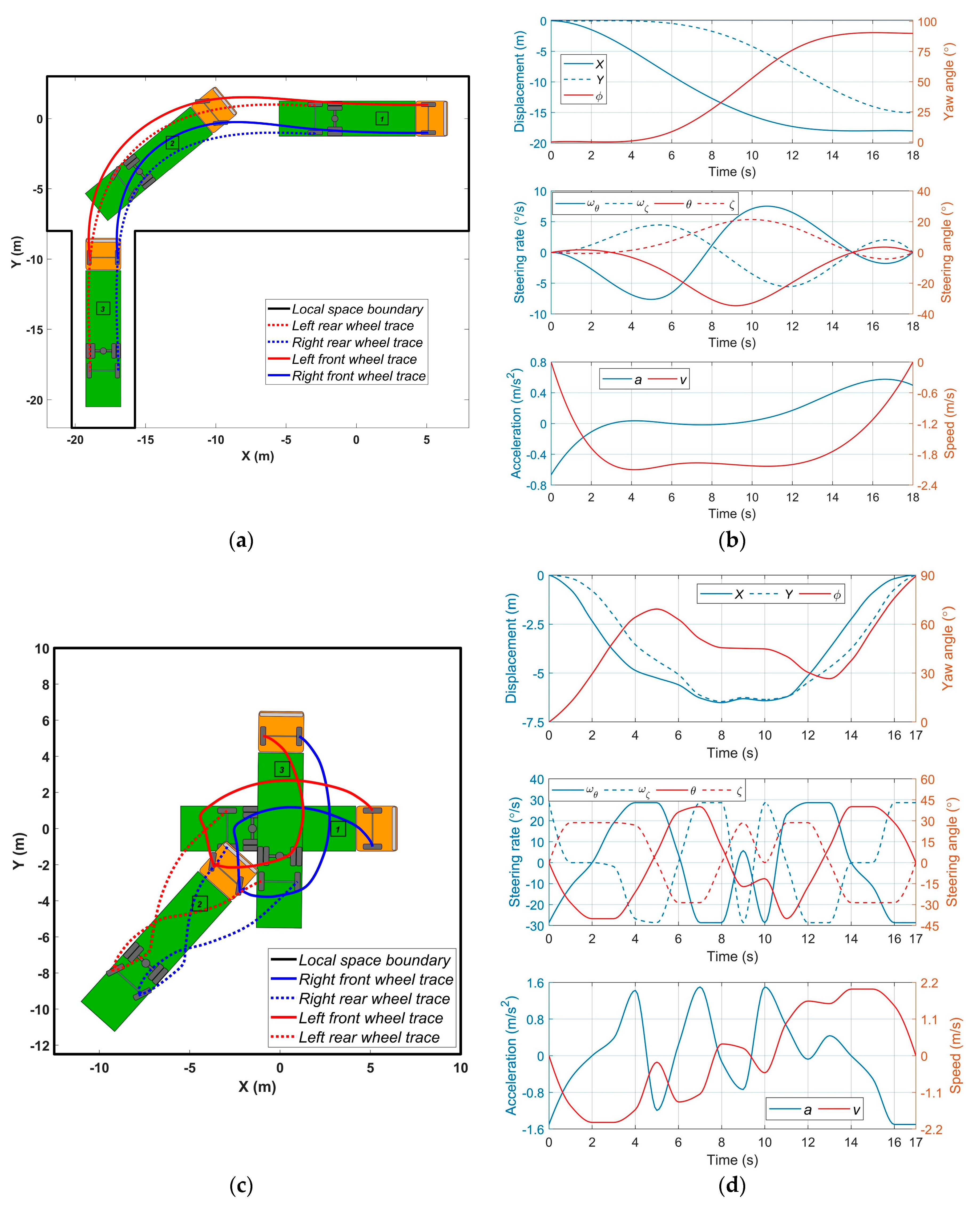
Figure 6.
Simulation results for the single truck circular motion: (a) Truck positions and planned trajectories; (b) Truck output and control parameters.
Figure 6.
Simulation results for the single truck circular motion: (a) Truck positions and planned trajectories; (b) Truck output and control parameters.

Figure 7.
Simulation results for the docking of articulated vehicles: (a) Position and trajectory (conventional TSV); (b) Basic parameters (conventional TSV); (c) Position and trajectory (TSV-SSA); (d) Basic parameters (TSV-SSA).
Figure 7.
Simulation results for the docking of articulated vehicles: (a) Position and trajectory (conventional TSV); (b) Basic parameters (conventional TSV); (c) Position and trajectory (TSV-SSA); (d) Basic parameters (TSV-SSA).

Figure 8.
Simulation results for the circular motion of articulated vehicles: (a) Position and trajectory (conventional TSV); (b) Basic parameters (conventional TSV); (c) Position and trajectory (TSV-SSA); (d) Basic parameters (TSV-SSA).
Figure 8.
Simulation results for the circular motion of articulated vehicles: (a) Position and trajectory (conventional TSV); (b) Basic parameters (conventional TSV); (c) Position and trajectory (TSV-SSA); (d) Basic parameters (TSV-SSA).

Table 1.
Restrictions and initial conditions for simulating passenger cars.
| Type of Motion | Restrictions 1 | Initial Conditions |
|---|---|---|
| Parallel reverse parking | −40 ° ≤ θ ≤ 40 °; −2 m/s ≤ v ≤ 2 m/s; −34 °/s ≤ ωθ ≤ 34 °/s; −1 m/s2 ≤ a ≤ 1 m/s2 | Ts = 1 s; p = 14; q0 = (0, 0, 0, 0, 0)T; qf = (−7.65, −5, 0, 0, 0)T |
| Perpendicular reverse parking | −40 ° ≤ θ ≤ 40 °; −2 m/s ≤ v ≤ 2 m/s; −34 °/s ≤ ωθ ≤ 34 °/s; −1 m/s2 ≤ a ≤ 1 m/s2 | Ts = 0.5 s; p = 14; q0 = (0, 0, 0, 0, 0)T; qf = (−5.5, −6.8, π/2, 0, 0)T |
| Perpendicular forward parking | −40 ° ≤ θ ≤ 40 °; −2 m/s ≤ v ≤ 2 m/s; −34 °/s ≤ ωθ ≤ 34 °/s; −1 m/s2 ≤ a ≤ 1 m/s2 | Ts = 1 s; p = 16; q0 = (0, 0, 0, 0, 0)T; qf = (−5.5, −6.8, −π/2, 0, 0)T |
| Circular motion 2,3 | −40 ° ≤ θ ≤ 40 °; Rout = 10 m, H = 2.3 m; Rin = Rout – H; −28 °/s ≤ ωθ ≤ 28 °/s; 0.95·vdes m/s ≤ v ≤ 1.25·vdes m/s; −2 m/s2 ≤ a ≤ 2.5 m/s2 | Ts = 1 s; p = 16; βC0 = −π·7/9; βCf = π·5/6; q0 = (Rav·cos(βC0), Rav·sin(βC0), π/2 +βC0, arctan(2·L/Rav), vdes)T; qf = (Rav·cos(βCf), Rav·sin(βCf), π/2 +βCf, arctan(2·L/Rav), vdes)T |
1vdes = 5 m/s (desirable circulating speed). 2 Rav = (Rout + Rin)/2. 3 Rav = (Rout + Rin)/k, where k = 2.15.
Table 2.
Restrictions and initial conditions for simulating long single trucks.
| Type of Motion | Restrictions 1 | Initial Conditions |
|---|---|---|
| Perpendicular reverse parking | −40° ≤ θ ≤ 40°; −30° ≤ ζ ≤ 30; −2 m/s ≤ v ≤ 2 m/s; −6 °/s ≤ ωθ ≤ 6 °/s; −6 °/s ≤ ωζ ≤ 6 °/s; −0.7 m/s2 ≤ a ≤ 0.7 m/s2 | Ts = 3 s; p = 6; q0 = (0, 0, 0, 0, 0, 0)T; qf = (−18, −15, π/2, 0, 0, 0)T |
| Parking with changing position on the spot | −40° ≤ θ ≤ 40°; −30° ≤ ζ ≤ 30; −2 m/s ≤ v ≤ 2 m/s; −28 °/s ≤ ωθ ≤ 28 °/s; −28 °/s ≤ ωζ ≤ 28 °/s; −1.5 m/s2 ≤ a ≤ 1.5 m/s2 | Ts = 1 s; p = 18; q0 = (0, 0, 0, 0, 0, 0)T; qf = (0, 0, π/2, 0, 0, 0)T |
| Circular motion 2,3 | −40° ≤ θ ≤ 40°; −30°≤ ζ ≤ 30°; 0.95·vdes m/s ≤ v ≤ 1.25·vdes m/s; Rout = 15 m, H = 4.5 m; Rin = Rout – H; −28 °/s ≤ ωθ ≤ 28 °/s; −28 °/s ≤ ωζ ≤ 28 °/s; −2 m/s2 ≤ a ≤ 2.0 m/s2 | Ts = 1 s; p = 13; βC0 = −135°; βCf = 140°; q0 = (Rav·cos(βC0), Rav·sin(βC0), π/2 +βC0, arctan(2·L10/Rav), −arctan(2·l10/Rav), vdes)T; qf = (Rav·cos(βCf), Rav·sin(βCf), π/2 +βCf, arctan(2· L10/Rav), −arctan(2·l10/Rav), vdes)T |
1vdes = 5 m/s (desirable circulating speed). 2 Rav = (Rout + Rin)/2. 3 Rav = (Rout + Rin)/k, where k = 2.15.
Table 3.
Restrictions and initial conditions for simulating articulated vehicles.
| Type of Automated Vehicle (AV) | Type of Motion | Restrictions 1 | Initial Conditions |
|---|---|---|---|
| Conventional TSV | Docking (unconstrained space) | −90° ≤ ψ ≤ 90°; −45° ≤ θ ≤ 45°; −4 m/s ≤ v ≤ 4 m/s; −34 °/s ≤ ωθ ≤ 34 °/s; −2.0 m/s2 ≤ a ≤ 2.5 m/s2 | Ts = 1 s; p = 12; q0 = (0, 0, π/2, 0, 0, 0)T; qf = (−5, −35, π, 0, 0, 0)T |
| Circular Motion 2 | Inequality constraint of Equation (56); Rout = 15 m, H = 5 m; Rin = Rout – H; −40° ≤ ψ ≤ 40°; −45° ≤ θ ≤ 45°; 0.95·vdes m/s ≤ v ≤ 1.25·vdes m/s; −34 °/s ≤ ωθ ≤ 34 °/s; −0.5 m/s2 ≤ a ≤ 0.5 m/s2 | Ts = 1 s; p = 9; βC0 = −160°; βCf = 140°; q0 = (Rav·cos(βC0), Rav·sin(βC0), π/2 +βC0, π·11/60, arctan(2·L1/Rav), vdes)T; qf = (Rav·cos(βCf), Rav·sin(βCf), π/2+βCf, π·11/60, arctan(2·L1/Rav), vdes)T | |
| TSV-SSA | Docking (unconstrained space) | −90° ≤ ψ ≤ 90°; −40° ≤ θ ≤ 40°; −35° ≤ ζ ≤ 35°; −4 m/s ≤ v ≤ 4 m/s; −34 °/s ≤ ωθ ≤ 34 °/s; −34 °/s ≤ ωζ ≤ 34 °/s; −2.0 m/s2 ≤ a ≤ 2.5 m/s2 | Ts = 1 s; p = 12; q0 = (0, 0, π/2, 0, 0, 0, 0)T; qf = (−5, −35, π, 0, 0, 0, 0)T |
| Circular motion 3 | Inequality constraint of Equation (56); Rout = 15 m, H = 4 m; Rin = Rout – H; 30° ≤ ψ ≤ 35°; 15° ≤ θ ≤ 20°; −15° ≤ ζ ≤ −10°; 0.95·vdes m/s ≤ v ≤ 1.05·vdes m/s; −34 °/s ≤ ωθ ≤ 34 °/s; −28 °/s ≤ ωζ ≤ 28 °/s; −0.5 m/s2 ≤ a ≤ 0.5 m/s2 | Ts = 1 s; p = 9; βC0 = -100; βCf = 200°; q0 = (Rav·cos(βC0), Rav·sin(βC0), π/2 +βC0, π/6, arctan(2·L1/Rav), -arctan(2·L1/Rav), vdes)T; qf = (Rav·cos(βCf), Rav·sin(βCf), π/2 +βCf, π/6, arctan(2·L1/Rav), -arctan(2·L1/Rav), vdes)T |
1vdes = 8 m/s (desirable circulating speed). 2 Rav = (Rout + Rin)/k, where k = 1.95. 3 Rav = (Rout + Rin)/k, where k = 2.025.
© 2020 by the authors. Licensee MDPI, Basel, Switzerland. This article is an open access article distributed under the terms and conditions of the Creative Commons Attribution (CC BY) license (http://creativecommons.org/licenses/by/4.0/).
Share and Cite
MDPI and ACS Style
Diachuk, M.; Easa, S.M.; Bannis, J. Path and Control Planning for Autonomous Vehicles in Restricted Space and Low Speed. Infrastructures 2020, 5, 42. https://doi.org/10.3390/infrastructures5050042
AMA Style
Diachuk M, Easa SM, Bannis J. Path and Control Planning for Autonomous Vehicles in Restricted Space and Low Speed. Infrastructures. 2020; 5(5):42. https://doi.org/10.3390/infrastructures5050042
Chicago/Turabian StyleDiachuk, Maksym, Said M. Easa, and Joel Bannis. 2020. "Path and Control Planning for Autonomous Vehicles in Restricted Space and Low Speed" Infrastructures 5, no. 5: 42. https://doi.org/10.3390/infrastructures5050042