Mixed Logic Dynamic Models for MPC Control of Wind Farm Hydrogen-Based Storage Systems
by
 ,
,
Muhammad Faisal Shehzad
1,*, 
Muhammad Bakr Abdelghany
1,
Davide Liuzza
2,
Valerio Mariani
1 and
Luigi Glielmo
1 1
Group for Research on Automatic Control Engineering, Department of Engineering, University of Sannio, Piazza Roma 21, 82100 Benevento, Italy
2
ENEA Fusion and Nuclear Safety Department, Via Enrico Fermi 45, 00044 Frascati (Rome), Italy
*
Author to whom correspondence should be addressed.
Inventions 2019, 4(4), 57; https://doi.org/10.3390/inventions4040057
Submission received: 10 August 2019
/
Revised: 11 September 2019
/
Accepted: 18 September 2019
/
Published: 26 September 2019
(This article belongs to the Special Issue Modeling, Planning and Optimal Management of Mini/Micro-Grid in Presence of Distributed Energy Resources)
Abstract
:The use of electric power by wind generation in actual grids is hampered by its inherent stochastic nature and the penalty deviations adopted in several electricity regulation markets with respect to power quality requirements. Coupling wind farms with advanced Energy Storage Systems (ESS) can help their integration within grids. In this direction, several studies have been conducted, but the problem is still open due to the constraints and limitations regarding the ESSs time autonomy, time response, degradation issues and overall costs. In order to take into account these relevant aspects, advanced control algorithms are needed. In this paper, a Model-Based Predictive Controller (MPC) is presented. Such a controller minimizes the degradation of the ESS and the load tracking error while fulfilling the operational constraints and dynamics. The ESS considered is hydrogen-based and the study has been developed within the EU-FCH 2 JU (European Union Fuel Cells and Hydrogen 2 Joint Undertaking) funded project HAEOLUS aiming at building and integrating advanced control strategies for a hydrogen-based ESS within a wind farm fence. Numerical simulations show the feasibility and the effectiveness of the proposed approach.
1. Introduction
Renewable energy sources are subjected to considerable attention for the replacement of fossil fuels. In particular, wind and solar energy are considered as the most promising options [1]. Many studies have been carried out to improve these technologies and to overcome the drawbacks associated with them. In particular, the stochastic nature of the wind, energy production and consumption mismatches and possibly high capital and operational cost are the main hurdles for their utilization at large scale [2].
One solution to mitigate these problems is to setup an energy storage system that can help the wind generation patterns in matching the load patterns along the time even in case of low or nearly zero energy production [2].
The adoption of an Energy Storage System (ESS) combined with a Renewable Energy System (RES) plant appears to be a paradigm shift in the energy market and introduces new operational possibilities [3,4]. However, the increased complexity of the plant itself requires proper management strategies. For this reason, control algorithms for Energy Management Systems (EMSs) have already been addressed in relevant works. Carapellucci et al. [5] presented a power management control strategy for assessing cost effective performances of renewable energy islands. Such controller also allows to include various electricity generation technologies into the hydrogen storage system. The hybridization of alternate energy sources with Fuel Cell (FC) systems using long and short-term storage strategies with appropriate power controllers and control strategies to meet the load demand has been presented by Uzunog et al. [6]. Castaneda et al. [7] implemented three control strategies to satisfy the load power demand, to regulate the state of charge of the batteries and to reduce the cost of battery cycling, FC and electrolyzer, respectively. Valverde et al. [8] implemented a supervisory Model Predictive Control (MPC) for hydrogen-based ESS for optimal power market management. Trifkovic et al. [9] implemented a hierarchical control system to track the dynamic load demand through the intermittent renewable energy generation and an energy storage. An MPC based on a mixed-integer quadratic programming algorithm was designed by Serna et al. [10] to improve the power balance between the available power and the electrolysis power consumption in an offshore plant using renewable energies.
The mixed-integer linear programming framework for wind–hydrogen plant modeling, including operational costs in the ESS, is used in [11,12,13,14] without integrating the degradation issues in the ESS. Vahidi et al. [15,16] applied the MPC to control the load sharing of a hybrid ESS composed of a fuel cell and an ultracapacitor, also including some degradation issues. However, these studies do not take into account the connection to the grid or the start-up/shutdown life cycles associated with the electrolyzer and the fuel cell.
Heuristic algorithms for degradation characterization with respect to the working hours/life cycles of the electrolyzer have been discussed by Bergen et al. [17]. Beside hydrogen-based storage, interesting control approaches for energy flow control in combined heat and power microgrids have been presented by Ferrari-Trecate et al. [18]. Also, the authors developed MPC for hybrid co-generation power plants by introducing a mixed linear dynamic framework [19].
The adoption of storage systems increases the complexity of the overall energy plants in terms of various aspects such as operational strategies, capital cost degradation, maintenance cost and efficiency reduction over time. Furthermore, each ESS technology introduces, together with more operational flexibility, peculiar limitations and constraints on the overall plant. Among the available technologies, the use of the hydrogen as an energy carrier can play an important role in the energy sector. For this reason, hydrogen storage system characteristics have been investigated in several studies, such as [20,21,22,23,24]. Several of them conclude that, among ESSs, the high energy density of the hydrogen may be beneficial in the new energetic paradigm. Hydrogen storage systems are composed of electrolyzers, fuel cells, and storage tanks. The optimal use of hydrogen storage requires the development of a control system, which takes into account all the constraints, limitations, degradation issues, and the economical cost in operating all the equipment. However, the robust performances and the transient responses associated to hydrogen-based ESS are considered as the main barriers in its utilization [25,26].
For all these reasons, in order to use the hydrogen-based ESSs efficiently, and operate them in the most effective way, the need of an advanced EMS is of paramount importance. The latter has to take into account all the operational constraints and limitations, as well as degradation, operational and maintenance cost in order to properly commit all the equipment and satisfy the energy demand profile. Aspects related to cost degradation and economical feasibility of hydrogen-based ESS have been addressed in [27].
Korpas et al. [28] implemented a MPC controller to integrate hydrogen ESS in the electrical market system but without accounting for the plant efficiency. Despite the valuable results of these papers, not all the aspects and constraints of both electrolyzer and fuel cells hydrogen-based ESS are considered at the same time.
According to the authors’ knowledge, important operational aspects of hydrogen-based storage systems such as degradation, mode operational switchings and stand by consumption of both electrolyzer and fuel cell have not been modeled in the literature. Our paper addresses such issues and develops preliminary operational models and constraints for a hydrogen-based ESS to be integrated in a wind farm fence under the EU-FCH JU project HAEOLUS—Hydrogen-Aeolic Energy with Optimized eLectrolysers Upstream of Substation [29].
Specifically, the plant is modeled considering Mixed Integer Linear (MIL) constraints for operating states and switchings and non linear dynamics for the hydrogen tank and the efficiency degradation rates. Also, depreciation cost are considered when switching among on (ON), off (OFF) and standby (STB) operational states. A controller is then derived whose goal is to track and meet the reference demand with the available system power at the best and in the most economical way. The designed MPC controller takes into account all the devices features here modeled and operates in reducing the operational and degradation cost of the devices while satisfying the constraints. Preliminary numerical results are conducted to show the effectiveness of our approach.
Nomenclature
2. System Description and Modeling
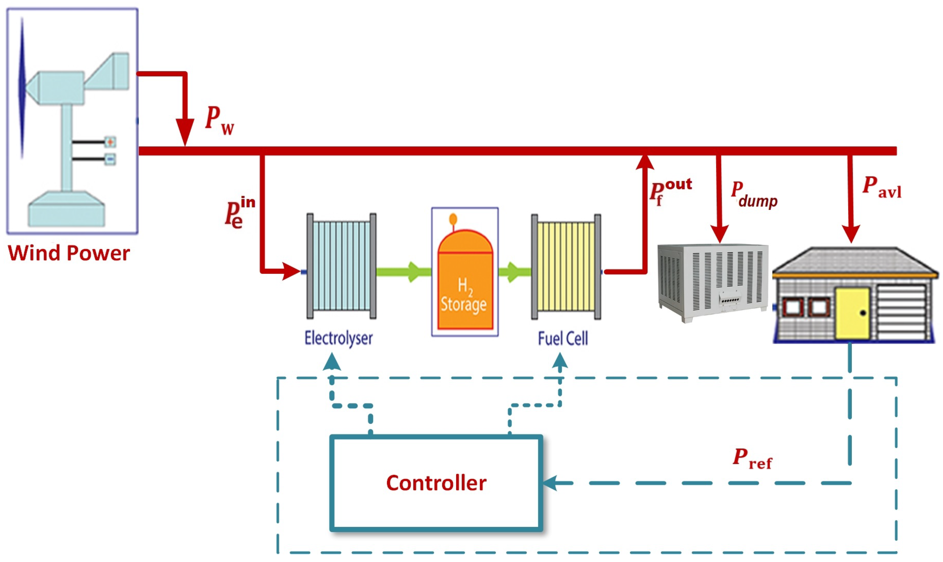
Figure 1 shows the block diagram of the system under investigation. Red solid lines denote energy flow, green solid lines denote hydrogen flows, and blue dashed lines denote data flows while denotes the power generated by the wind farm, is the electrolyzer input power, is the fuel cell output power, is the power that can be dissipated on a dumping load and is the power available to the load. Dumping of the wind power excess is usually necessary if the power surplus exceeds the transmission capacity of the external grid. However, in the case under investigation the dumping load may be conveniently exploited to mitigate the degradation of the electrolyzer, therefore helping to mitigate the impact of the corresponding operational costs.
In nominal conditions, is delivered directly to the load demand. However, when an excess of wind power production happens, this is shunted to the electrolyzer and stored as hydrogen in a tank. Conversely, whenever the generated wind power can not satisfy the load demand, the hydrogen is then re-electrified through the fuel cell, thus achieving power supply continuity.
2.1. Power Demand Reference Model
In our scenario, the power demand reference is forecasted by an external system, fed into the MPC controller and then used within a tracking error cost function.
2.2. Electrolyzer and Fuel Cell Models
The electrolyzer and the fuel cell have been both modeled as a three states automaton, as shown in Figure 2. For each one, the three possible states are on (ON), off (OFF) and standby (STB). Correspondingly, the mutually exclusive logical variables , with and , are used to indicate the operating conditions of the electrolyzer and the fuel cell at any time k.
More in detail, each operational state of the electrolyzer and the fuel cell results in a particular product of one logical variable and one corresponding power, which is relevant for that state, to be different from zero. For example, whenever the electrolyzer or the fuel cell is in ON state, the corresponding input or output power is limited within the range . Thus, by defining and , and since in this case we set , then it results and . Moreover, being by defition mutually exclusive for each , all other logical variables are null, instead. On the other hand, whenever the electrolyzer or the fuel cell is in STB state, the relevant powers to be considered are their corresponding stand-by powers , with . Therefore, by defining and it follows that and since accordingly , while, again, all other logical variables are null. Finally, when the electrolyzer or the fuel cell is in OFF state, their corresponding input or output powers along with the power consumptions are null, resulting in . Therefore, according to the operating condition of the electrolyzer and of the fuel cell, each with is determined at any time k as follows
Along with the logical states, also the feasible state transitions among them have to be modeled. To this aim we need the additional logical variables , with , and which can be derived by suitably combining the logical states through logical connectives. The transition variables assume value if the corresponding transition happens at time k (available transitions are depicted in Figure 2), while null value otherwise. It is important to notice that s and s are 18 decision variables of the MPC controller that will be presented later. Both state variables and transition variables are codified with mixed integer linear inequalities which will be then included as constraints for the MPC controller. The mathematical formulation of these constraints is reported, for the reader convenience, in the Appendix A.
2.3. Hydrogen Storage Model
The hydrogen storage dynamics are defined as a function of the hydrogen level at the previous time step [25]. The and , are respectively, the efficiency degradations of the electrolizer and of the fuel cell, respectively, and have been modeled as dynamic equations since they change along the time
where is the degradation rate at the maximum power [30] and over the number of yearly life hours of the electrolyzer () and of the fuel cell (), with is the number of the per year life hours of the electrolyzer () and of the fuel cell () and denotes the sampling period. Notice that, according to (2), the electrolyzer and the fuel cell produces and consumes hydrogen only in their ON modes. All the other modes are not associated with the hydrogen production and consumption respectively and, therefore, are not associated to efficiency degradation.
2.4. Feasibility and Operating Constraints
In addition to the constraints due to the considered dynamics, it is necessary to take into account also for the subsystems physical limitations. In fact, the actual ESS can absorb or supply just a limited amount of power. Further, also the power that can be dissipated by the dumping load cannot exceed a limit, which in our case is set to be the power achieved by wind generation
2.5. Power Balance Constraint
The available power , which is delivered to the load, is obtained by forcing the power balance at the ESS insertion point
where and = . The power balance (4) highlights that the available power depends on the power achieved through wind generation and the balancing action of the hydrogen storage system and the dumping load.
3. Implementation of the Proposed MPC Controller
In this section we illustrate the MPC control strategy that has been designed to optimize the problem of satisfying a forecasted power demand in the most economical way [31,32]. The main idea of the MPC is to exploit the model of the plant to predict the future evolution of the system within a prediction horizon. Based on this prediction, at each step k the controller selects a sequence of future command inputs through an optimization procedure, which aims at minimizing a suitable cost function and enforcing the fulfillment of the constraints. Only the control signal calculated for the time instant k is applied to the process. At the next sampling time, the new state of the system is measured or estimated, and a new optimization problem is solved using this new information. The introduction of logical variables makes the system as a mixed logical dynamical system. One of the advantages of MPC over other control methods is its immediate applicability to multivariable control systems.
3.1. Electrolyzer and Fuel cell Cost Functions
The cost incurred in operating the electrolyzer and the fuel cell are summarized in the two respective cost functions derived in this section. Both of them are expressed as a summation of different cost related to the component depreciation, the reduction in the number of life cycles and the energy spent in keeping the units warm during the stand by mode. More in details, the manufacturers of the electrolyzer and the fuel cell defined the life cycles of the devices as a function of number of working hours. It has been noticed in many studies [33,34,35,36,37] that the fluctuating loads and the operating cycles can seriously affect these devices in a number of ways. Therefore, in order to tackle such outlined problems, we propose the following cost
where and denote the operating and maintenance cost of the electrolyzer and the fuel cell, is the power spot price, is the number of life hours of the electrolyzer and is the number of life hours of the fuel cell. , , , , , and describe the startup, shutdown and standby cost of the electrolyzer and the fuel cell, respectively choosing . These cost are payed any time a mode switch occurs, since any complete sequence of switching accounts for a working cycle and, therefore, reduces the components’ life. We wish to emphasize, for the sake of clarity, that shifting from OFF to ON (cold start) presents usually a higher cost than from STB to ON (warm start). On the other hand, devices in OFF mode do not absorb any power, while this is not true in STB mode. The and represent the stack replacement cost of the electrolyzer and the fuel cell, respectively.
3.2. Load Tracking Cost Function
In addition to the minimization of the operating costs of the electroyzer and the fuel cell, the other goal is to track a reference load demand , that in the scenario under investigation is forecasted. To this aim, the corresponding cost function which will be included in the optimization is given by the square error between the available power downstream the ESS and the forecasted load demand
3.3. MPC Formulation
In order to present the MPC policy, let us just consider the hydrogen dynamics in (2) and let us denote by , and , with , the corresponding state variables at time predicted at time k by means of (2) as well.
At each k, given the initial state , and , the MPC provides the optimal control sequences and for each , , and , and where
by solving
with being , and some weights. Since the problem (8) is re-formulated at time , an optimal feedback policy is designed.
Summarizing, the following objectives have been explicitly taken into account:
- protection of the hydrogen storage tank from excessive discharging and overcharging;
- limitation of the power rate of the fuel cell and of the electrolyzer to protect them;
- tracking of the power reference request according to the forecasted conditions;
- in case an expected event occurs, the fuel cell is employed as a contingent energy storage system to satisfy the power demand.
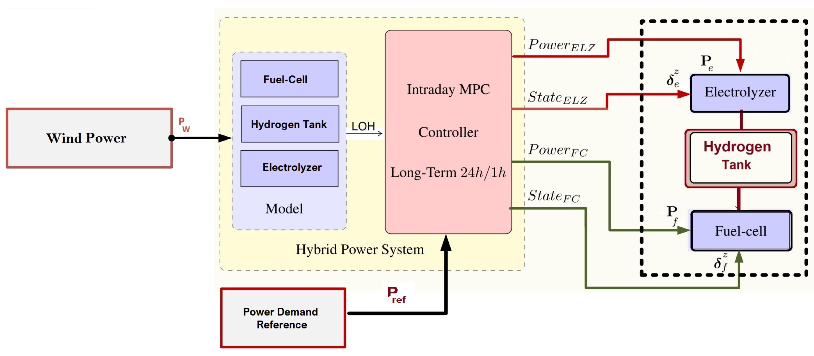
The block diagram of the proposed controller is detailed in Figure 3. and represent the discrete states of the electrolyzer and the fuel cell, where indexes their logical states.
4. Case Study
The model of the proposed EMS consisting of discrete operational states of the electrolyzer and of the fuel cell, the corresponding MLD constraints and the continuous dynamics have been implemented using MATLAB/YALMIP. The controller was implemented using the solver ILOG’s CPLEX 12.8; all computations are performed on a laptop with an Intel Core (TM) HQ 2.8 GHz processor and 16 GB of memory. Optimization results are obtained in less than 1 minute. The MPC is tuned mainly penalizing the electrolyzer and the fuel cell cost functions with respect to the load tracking one. In order to finalize the controller setup, the prediction horizon is with sampling time . The cost values considered in our study are reported in Table 4. The switching cost for the standby state of both devices is lower in comparison with OFF to ON or ON to OFF states. The advantage of keeping the devices to their standby states is to avoid their cold start, and so a lower cost has to be paid for state switching. However, on the other hand the constant = power is supplied to both devices to keep them in their standby state. The electrolyzer and of the fuel cell degradation rates are both set to , with , and the stack replacement cost of the electrolyzer () and of the fuel cell () have been determined according to
where , for each , is reported in Table 4 as well as other used values. Also, the considered initial conditions for efficiency degradations and are and , respectively.
The degradation factor considered in this study is provided by the developer and the manufacturer of the PEM technology electrolyzer and the fuel cell [30]. Since the HAEOLUS project (the one founding our research and studied in the manuscript) is in its first year and will end in 2022, better degradation factors will be considered leveraging on the working plan data (up to now, the site is under construction).
5. Simulations and Numerical Results
5.1. Example 1
The main contribution of this paper relies in the derivation of preliminary operating models needed for running the hydrogen-based ESS for long control periods as being implemented within the EU-FCH 2 JU funded project HAEOLUS [29]. However, in order to test the system, a power demand tracking is considered. The tuning of the load tracking cost function weights seeks for a soft tracking of the output variables towards the given references and an efficient use of the energy. More specifically, if there exists a big difference between the demanded energy and the energy by wind generation, the controller operates the ESS in order to track the demand however with a major preference for minimizing operating costs. Accordingly, the prioritization weights , and have been adjusted by trial and error. In the simulations, is considered as the initial level of the hydrogen in the tank.
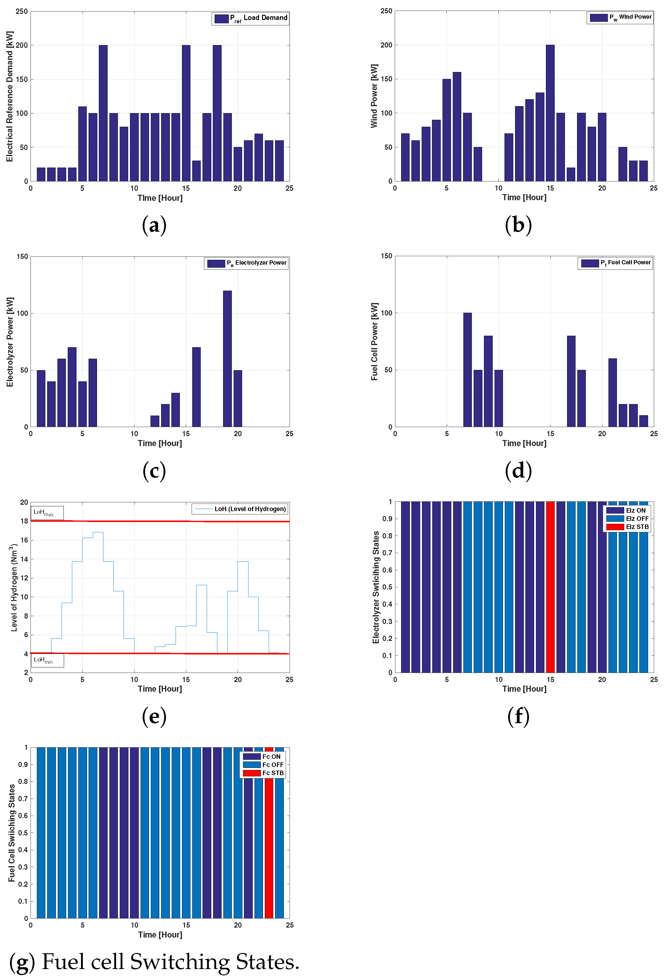
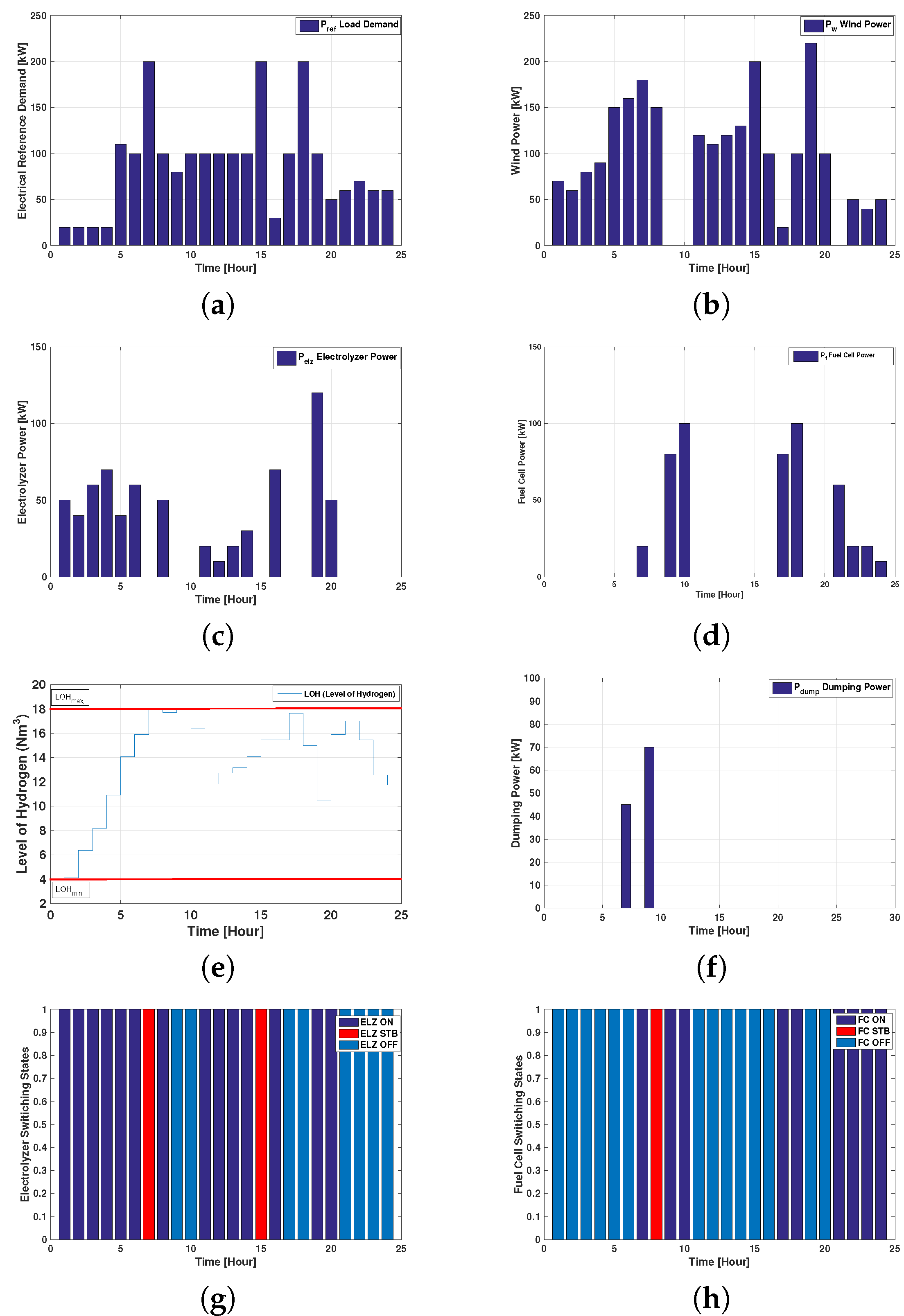
In our numerical examples, the wind power production and the reference power demand are such that both exceeding and missing power are considered, with a power flow towards or from the storage. In order to show the effectiveness of the implemented algorithm, the devices switching states have been shown for a case with frequent imbalances between the reference demand and the wind power over the 24 h simulation. Figure 4a,b show the electrical reference demand and the wind power , respectively. It can be seen that the difference between the wind power and the reference demand is positive for the first 6 h, so the reference demand is met through the wind power only and the exceeding power is shunted to the electrolyzer (which was set by the controller to its ON state) for hydrogen production according to the current level of hydrogen and the physical constraints of the storage (Figure 4c). Figure 4e shows that the level of hydrogen in the storage has increased according to the storage constraints from to during the excess wind hours. Figure 4d shows the fuel cell power. It can be clearly observed from Figure 4d that the fuel cell does not supply power (in its OFF state) to the load when the wind power availability is higher than the reference demand. It is important to note that the controller is designed to switch the electrolyzer and the fuel cell to their STB state if it predicts the need to switch them on again in the near future, i.e., hours 7 and 15 for the electrolyzer and hour 8 for the fuel cell. Figure 4g,h show the switching states of the electrolyzer and the fuel cell, respectively. On the other hand, during the hours when the demand is higher than the wind power production (that even falls at zero for hours 9–10 and 21). The fuel cell provides back up power for re-electrification, switching from OFF to ON states. The needed power is so provided by the previously stored hydrogen in the tank. The opposite, instead, happens to the electrolyzer since there is not enough power to be stored Figure 4c. Dumping of excess wind power is necessary when the power surplus exceeds the storage capacity of the hydrogen tank and the transmission capacity of the external grid. Figure 4f shows that the load is being dumped during hours 7 and 9. The power surplus during these hours cannot be stored into the storage tank since the hydrogen level has already reached the tank upper bound constraint (3).
5.2. Example 2
In order to show the effectiveness of the implemented algorithm, a stressing plant scenario has been considered in this example. As discussed above, the goal of the study is to track the reference power as much as possible with . In the case considered, the power is lower than the load demand , and the controller will only be able to deliver what is available in the system, which necessarily leads to a poor performance in meeting the desired requested power .
The load demand and the wind power profiles considered in this example are shown in Figure 5a,b, respectively. Figure 5c,d show the electrolyzer and the fuel cell powers for hydrogen production and consumption over the 24 h simulation horizon. It can be clearly observed from Figure 5e that during the hours 10, 11 and 18, the hydrogen in the tank is at its minimum threshold because of low or nearly zero wind power availability. So, the power available in the system is less than the power needed to meet the desired load demand for the said hours. This higher requested load demand can not be fully met, which results in system poor performance. Still, even in this case, the MPC controller guarantees optimal performances without violating hard physical constraints. The electrolyzer and the fuel cell switching states are shown in Figure 5f,g, respectively. Notice also that no dumping load has been observed in this scenario, because the hydrogen level has not exceeded the maximum threshold .
6. Conclusions
In this work, we developed models for operating, with optimal control strategies, a hydrogen-based energy storage system to be coupled to a wind farm. The models both encode discrete logical states representing operating device modes and continuous dynamics. The cost functions take into account the cost that each device introduces any time it switches between logical states, thus decreasing the number of life cycles and degrading the efficiency along its working conditions. Furthermore, all other physical constraints and costs, such as the power consumption in standby mode, are considered. The cost related to each device and the models developed will then be included in a suitable control architecture and implemented on a real wind farm under the EU-FCH 2 JU project HAEOLUS [29]. To preliminary test the proposed models, in this paper we considered a power demand reference tracking goal over an optimization horizon of 24 h. Numerical results show the correct behavior of the devices and their switching among the different operating modes. The power is correctly stored or retrieved via hydrogen conversion to help the wind production in determine the total available power and match the power requests.
Author Contributions
Conceptualization, D.L.; methodology, M.F.S., M.B.A. and D.L.; software, M.F.S. and M.B.A.; validation, M.F.S. and M.B.A.; investigation, D.L. and V.M.; resources L.G.; writing—original draft preparation, M.F.S.; writing—review and editing, D.L., V.M. and L.G.; supervision, D.L., V.M. and L.G.; project administration, D.L. and V.M.; funding acquisition, L.G.
Funding
This work received funding from the Fuel Cells and Hydrogen 2 Joint Undertaking under the project HAEOLUS, grant agreement No. 779469 https://www.haeolus.eu.
Conflicts of Interest
The authors declare no conflicts of interest.
Appendix A.
Appendix A.1. Constraints Formulation of the Logical States
In order to cope with an optimal control framework we need to introduce 12 auxiliary Boolean variables , with and [40]
Then, (A1) can be expressed as
where M is a sufficiently large positive number.
The auxiliary variables codified by the inequalities (A2) are then exploited to model the Mixed-Linear Dynamic (MLD) by linking the discrete logical variables of each device with the corresponding operating power, according to (1). Namely, for , , the variables are determined by
Notice that, despite being continuous, they can only assume the binary values due to (A3), that is in practice s are logical.
Appendix A.2. Mathematical Model and Constraints Formulation of the State Transitions
As discussed above, the devices models are characterized by three discrete operational states. These operational states imply possible mode transitions for each device. In what follows, we define all of the transitions. The transitions among the states for the each transition is the result of the state change, and can be defined by suitably combining logical variables, thus achieving
with , , . Using the relationships defined by Bemporad and Morari [40], each expression of the (A4) is equivalently converted into three inequalities and introduced in the constraints of MPC controller, thus resulting in the 18 following formulas
where , and analogously to s, they can only assume values due to (A5).
References
- Hosseini, S.E.; Wahid, M.A. Hydrogen production from renewable and sustainable energy resources: Promising green energy carrier for clean development. Renew. Sustain. Energy Rev. 2016, 57, 850–866. [Google Scholar] [CrossRef]
- Tande, J.O.G. Exploitation of wind-energy resources in proximity to weak electric grids. Appl. Energy 2000, 65, 395–401. [Google Scholar] [CrossRef]
- Akinyele, D.; Rayudu, R. Review of energy storage technologies for sustainable power networks. Sustain. Energy Technol. Assess. 2014, 8, 74–91. [Google Scholar] [CrossRef]
- Schoenung, S.M. Characteristics and Technologies for Long-vs. Short-Term Energy Storage; United States Department of Energy, Sandia National Laboratories: Albuquerque, NM, USA, 2001.
- Carapellucci, R.; Giordano, L. Modeling and optimization of an energy generation island based on renewable technologies and hydrogen storage systems. Int. J. Hydrogen Energy 2012, 37, 2081–2093. [Google Scholar] [CrossRef]
- Uzunoglu, M.; Onar, O.; Alam, M. Modeling, control and simulation of a PV/FC/UC based hybrid power generation system for stand-alone applications. Renew. Energy 2009, 34, 509–520. [Google Scholar] [CrossRef]
- Castaneda, M.; Cano, A.; Jurado, F.; Sánchez, H.; Fernandez, L.M. Sizing optimization, dynamic modeling and energy management strategies of a stand-alone PV/hydrogen/battery-based hybrid system. Int. J. Hydrogen Energy 2013, 38, 3830–3845. [Google Scholar] [CrossRef]
- Valverde, L.; Bordons, C.; Rosa, F. Power management using model predictive control in a hydrogen-based microgrid. In Proceedings of the IECON 38th Conference on Industrial Electronics Society, Montreal, QC, Canada, 25–28 October 2012; pp. 5669–5676. [Google Scholar]
- Trifkovic, M.; Sheikhzadeh, M.; Nigim, K.; Daoutidis, P. Hierarchical control of a renewable hybrid energy system. In Proceedings of the IEEE 51st Conference on Decision and Control (CDC), Grand Wailea, Maui, HI, USA, 16 August 2012; pp. 6376–6381. [Google Scholar]
- Serna, Á.; Yahyaoui, I.; Normey-Rico, J.E.; de Prada, C.; Tadeo, F. Predictive control for hydrogen production by electrolysis in an offshore platform using renewable energies. Int. J. Hydrogen Energy 2017, 42, 12865–12876. [Google Scholar] [CrossRef]
- De Angelis, F.; Boaro, M.; Fuselli, D.; Squartini, S.; Piazza, F.; Wei, Q. Optimal home energy management under dynamic electrical and thermal constraints. IEEE Trans. Ind. Inform. 2013, 9, 1518–1527. [Google Scholar] [CrossRef]
- Jiang, Q.; Xue, M.; Geng, G. Energy management of microgrid in grid-connected and stand-alone modes. IEEE Trans. Power Syst. 2013, 28, 3380–3389. [Google Scholar] [CrossRef]
- Yang, P.; Nehorai, A. Joint optimization of hybrid energy storage and generation capacity with renewable energy. IEEE Trans. Smart Grid 2014, 5, 1566–1574. [Google Scholar] [CrossRef]
- Malysz, P.; Sirouspour, S.; Emadi, A. An optimal energy storage control strategy for grid-connected microgrids. IEEE Trans. Smart Grid 2014, 5, 1785–1796. [Google Scholar] [CrossRef]
- Vahidi, A.; Greenwell, W. A decentralized model predictive control approach to power management of a fuel cell-ultracapacitor hybrid. In Proceedings of the 2007 American Control Conference, New York, NY, USA, 11–13 July 2017; pp. 5431–5437. [Google Scholar]
- Greenwell, W.; Vahidi, A. Predictive control of voltage and current in a fuel cell–ultracapacitor hybrid. IEEE Trans. Ind. Electron. 2009, 57, 1954–1963. [Google Scholar] [CrossRef]
- Bergen, A.P. Integration and Dynamics of a Renewable Regenerative Hydrogen Fuel Cell System. Ph.D. Thesis, University of Victoria, Victoria, BC, Canada, 25 April 2008. [Google Scholar]
- Ferrari-Trecate, G.; Gallestey, E.; Letizia, P.; Spedicato, M.; Morari, M.; Antoine, M. Modeling and control of co-generation power plants: A hybrid system approach. IEEE Trans. Control Syst. Technol. 2004, 12, 694–705. [Google Scholar] [CrossRef]
- Ferrari-Trecate, G.; Gallestey, E.; Letizia, P.; Spedicato, M.; Morari, M.; Antoine, M. Modeling and Control of Co-Generation Power Plants: A Hybrid System Approach; Tomlin, C.J., Greenstreet, M.R., Eds.; Hybrid Systems: Computation and Control; Springer: Berlin/Heidelberg, Germany, 2002; pp. 209–224. [Google Scholar]
- Stevens, M. Hybrid Fuel Cell Vehicle Power Train Development Considering Power Source Degradation. Ph.D. Thesis, University of Waterloo, Waterloo, ON, Canada, 2009. [Google Scholar]
- Vazquez, S.; Lukic, S.M.; Galvan, E.; Franquelo, L.G.; Carrasco, J.M. Energy storage systems for transport and grid applications. IEEE Trans. Ind. Electron. 2010, 57, 3881–3895. [Google Scholar] [CrossRef]
- Tani, A.; Camara, M.B.; Dakyo, B. Energy management based on frequency approach for hybrid electric vehicle applications: Fuel-cell/lithium-battery and ultracapacitors. IEEE Trans. Veh. Technol. 2012, 61, 3375–3386. [Google Scholar] [CrossRef]
- Wang, L.; Li, H. Maximum fuel economy-oriented power management design for a fuel cell vehicle using battery and ultracapacitor. IEEE Trans. Ind. Appl. 2010, 46, 1011–1020. [Google Scholar] [CrossRef]
- Liu, W.S.; Chen, J.F.; Liang, T.J.; Lin, R.L.; Liu, C.H. Analysis, design, and control of bidirectional cascoded configuration for a fuel cell hybrid power system. IEEE Trans. Power Electron. 2010, 25, 1565–1575. [Google Scholar]
- Garcia-Torres, F.; Valverde, L.; Bordons, C. Optimal load sharing of hydrogen-based microgrids with hybrid storage using model-predictive control. IEEE Trans. Ind. Electron. 2016, 63, 4919–4928. [Google Scholar] [CrossRef]
- Kalinci, Y.; Hepbasli, A.; Dincer, I. Techno-economic analysis of a stand-alone hybrid renewable energy system with hydrogen production and storage options. Int. J. Hydrogen Energy 2015, 40, 7652–7664. [Google Scholar] [CrossRef]
- Geer, T.; Manwell, J.; McGowan, J. A feasibility study of a wind/hydrogen system for Martha’s Vineyard, Massachusetts. In Proceedings of the American Wind Energy Association Windpower 2005 Conference; Massachusetts Technology Corporation (MTC): Brighton, MA, USA, 2005; Volume 37. [Google Scholar]
- Korpas, M. Distributed Energy Systems with Wind Power and Energy Storage. Ph.D. Thesis, Norwegian University of Science and Technology, Trondheim, Norway, 2004. [Google Scholar]
- Hydrogen-Aeolic Energy with Optimized Electrolysers Upstream of Substatio Project. 2018. Available online: http://www.haeolus.eu/ (accessed on 20 July 2019).
- Hydrogenics—Innovators in Hydrogen Technology & Solutions. 1995. Available online: http://www.hydrogenics.com/ (accessed on 2 September 2019).
- Parisio, A.; Rikos, E.; Glielmo, L. A model predictive control approach to microgrid operation optimization. IEEE Trans. Control Syst. Technol. 2014, 22, 1813–1827. [Google Scholar] [CrossRef]
- Alessandra, P.; Glielmo, L. Energy Efficient Microgrid Management using Model Predictive Control. In Proceedings of the 50th IEEE Conference on Decision and Control and European Control Conference (CDC-ECC), Orlando, FL, USA, 12–15 Decemeber 2011. [Google Scholar]
- Alavi, F.; Lee, E.P.; van de Wouw, N.; De Schutter, B.; Lukszo, Z. Fuel cell cars in a microgrid for synergies between hydrogen and electricity networks. Appl. Energy 2017, 192, 296–304. [Google Scholar] [CrossRef] [Green Version]
- Petrollese, M.; Valverde, L.; Cocco, D.; Cau, G.; Guerra, J. Real-time integration of optimal generation scheduling with MPC for the energy management of a renewable hydrogen-based microgrid. Appl. Energy 2016, 166, 96–106. [Google Scholar] [CrossRef]
- Khalid, M.; Savkin, A. A model predictive control approach to the problem of wind power smoothing with controlled battery storage. Renew. Energy 2010, 35, 1520–1526. [Google Scholar] [CrossRef]
- Olatomiwa, L.; Mekhilef, S.; Ismail, M.; Moghavvemi, M. Energy management strategies in hybrid renewable energy systems: A review. Renew. Sustain. Energy Rev. 2016, 62, 821–835. [Google Scholar] [CrossRef]
- Núñez-Reyes, A.; Rodríguez, D.M.; Alba, C.B.; Carlini, M.Á.R. Optimal scheduling of grid-connected PV plants with energy storage for integration in the electricity market. Sol. Energy 2017, 144, 502–516. [Google Scholar] [CrossRef]
- Spendelow, J.; Marcinkoski, J.; Satyapal, S. Doe hydrogen and fuel cells program record 14012. Dep. Energy (DOE) 2014, 125. Available online: https://www.hydrogen.energy.gov/pdfs/14012_fuel_cell_system_cost_2013.pdf (accessed on 13 June 2014).
- Howel, D. Battery status and cost reduction prospects. In EV everywhere grand challenge battery workshop. Dep. Energy (DOE) 2012, 125. Available online: https://www1.eere.energy.gov/vehiclesandfuels/pdfs/ev_everywhere/5_howell_b.pdf (accessed on 26 July 2012).
- Bemporad, A.; Morari, M. Control of systems integrating logic, dynamics, and constraints. Automatica 1999, 35, 407–427. [Google Scholar] [CrossRef]
Figure 1.
Block diagram of the microgrid under investigation. , , , and are the power by wind generation, the power inward the electrolyzer, the power outward the fuel cell, the power demand reference and the dumped power, respectively.
Figure 1.
Block diagram of the microgrid under investigation. , , , and are the power by wind generation, the power inward the electrolyzer, the power outward the fuel cell, the power demand reference and the dumped power, respectively.

Figure 2.
Automata of the electrolyzer () and of the fuel cell (). Each node represents a particular state (i.e., operational mode), while the edges represent the state transition, for each .
Figure 2.
Automata of the electrolyzer () and of the fuel cell (). Each node represents a particular state (i.e., operational mode), while the edges represent the state transition, for each .
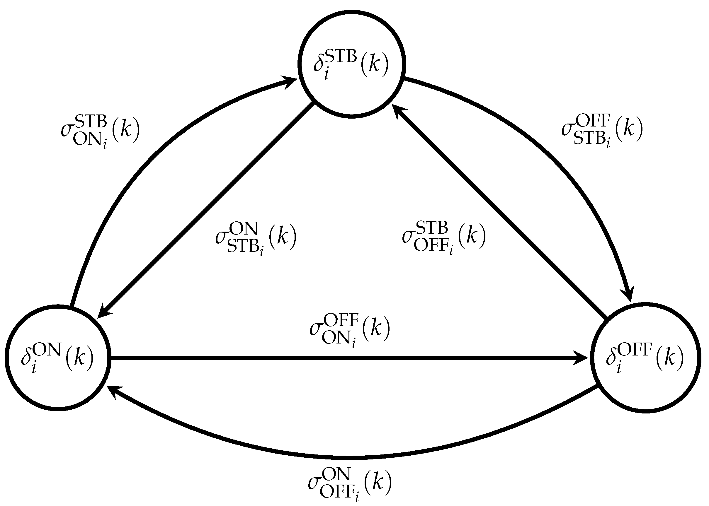
Figure 3.
Proposed MPC Control Scheme.

Figure 4.
Numerical results for Example 1. (a) Electrical Reference Demand. (b) Forecasted Wind Power. (c) Power of the Electrolyzer. (d) Power of the Fuel Cell. (e) Level of Hydrogen. (f) Dump Load. (g) Electrolyzer Switching States. (h) Fuel cell Switching States.
Figure 4.
Numerical results for Example 1. (a) Electrical Reference Demand. (b) Forecasted Wind Power. (c) Power of the Electrolyzer. (d) Power of the Fuel Cell. (e) Level of Hydrogen. (f) Dump Load. (g) Electrolyzer Switching States. (h) Fuel cell Switching States.

Figure 5.
Numerical results for Example 2. (a) Electrical Reference Demand. (b) Forecasted Wind Power. (c) Power of the Electrolyzer. (d) Power of the Fuel Cell. (e) Level of Hydrogen. (f) Electrolyzer Switching States. (g) Fuel cell Switching States.
Figure 5.
Numerical results for Example 2. (a) Electrical Reference Demand. (b) Forecasted Wind Power. (c) Power of the Electrolyzer. (d) Power of the Fuel Cell. (e) Level of Hydrogen. (f) Electrolyzer Switching States. (g) Fuel cell Switching States.

Table 1.
Parameters.
| Parameters | Description |
|---|---|
| Hydrogen level in the storage unit [Nm3] | |
| Maximum level of the hydrogen storage unit [Nm3] | |
| Minimum level of the hydrogen storage unit [Nm3] | |
| Maximum power level of the electrolyzer [] | |
| Standby power of the electrolyzer [] | |
| Minimum power level of the electrolyzer [] | |
| Maximum power level of the fuel cell [] | |
| Minimum power level of the fuel cell [] | |
| Standby power of the fuel cell [] | |
| Number of life hours of the electrolyzer | |
| Number of life hours of the fuel cell | |
| Number of per year life hours of the electrolyzer | |
| Number of per year life hours of the fuel cell | |
| Degradation rate of the electrolyzer at maximum input power and over the number of yearly life hours | |
| Degradation rate of the fuel cell at maximum output power and over the number of yearly life hours | |
| Electrolyzer stack replacement cost [€/] | |
| Fuel cell stack replacement cost [€/] | |
| Sampling period [] | |
| T | Simulation horizon [] |
Table 2.
Forecast powers.
| Forecasts | Description |
|---|---|
| Wind power production [] | |
| Electrical load demand [] |
Table 3.
Real and logical time varying variables.
| Variables | Description |
|---|---|
| On state of the electrolyzer | |
| Off state of the electrolyzer | |
| Standby state of the electrolyzer | |
| On state of the fuel cell | |
| Off state of the fuel cell | |
| Standby state of the fuel cell | |
| Electrical power of the electrolyzer [] | |
| Electrical power of the fuel cell [] | |
| Available system electrical power [] | |
| Dumped electrical power [] | |
| z | Electric power formulated as mixed logic dynamic (MLD) variables for the electrolyzer and the fuel cell [] |
| Logical variables ON/OFF/STB states for the electrolyzer and the fuel cell | |
| Electrolyzer degradation rate [Nm3/] | |
| Fuel cell degradation rate [/Nm3] |
© 2019 by the authors. Licensee MDPI, Basel, Switzerland. This article is an open access article distributed under the terms and conditions of the Creative Commons Attribution (CC BY) license (http://creativecommons.org/licenses/by/4.0/).
Share and Cite
MDPI and ACS Style
Shehzad, M.F.; Abdelghany, M.B.; Liuzza, D.; Mariani, V.; Glielmo, L. Mixed Logic Dynamic Models for MPC Control of Wind Farm Hydrogen-Based Storage Systems. Inventions 2019, 4, 57. https://doi.org/10.3390/inventions4040057
AMA Style
Shehzad MF, Abdelghany MB, Liuzza D, Mariani V, Glielmo L. Mixed Logic Dynamic Models for MPC Control of Wind Farm Hydrogen-Based Storage Systems. Inventions. 2019; 4(4):57. https://doi.org/10.3390/inventions4040057
Chicago/Turabian StyleShehzad, Muhammad Faisal, Muhammad Bakr Abdelghany, Davide Liuzza, Valerio Mariani, and Luigi Glielmo. 2019. "Mixed Logic Dynamic Models for MPC Control of Wind Farm Hydrogen-Based Storage Systems" Inventions 4, no. 4: 57. https://doi.org/10.3390/inventions4040057