Underwater Soundscape Monitoring and Fish Bioacoustics: A Review


Department of Biology, Boston University, 5 Cummington Mall, Boston, MA 02215, USA
*
Authors to whom correspondence should be addressed.
Fishes 2018, 3(3), 36; https://doi.org/10.3390/fishes3030036
Submission received: 10 August 2018
/
Revised: 5 September 2018
/
Accepted: 6 September 2018
/
Published: 12 September 2018
Abstract
:Soundscape ecology is a rapidly growing field with approximately 93% of all scientific articles on this topic having been published since 2010 (total about 610 publications since 1985). Current acoustic technology is also advancing rapidly, enabling new devices with voluminous data storage and automatic signal detection to define sounds. Future uses of passive acoustic monitoring (PAM) include biodiversity assessments, monitoring habitat health, and locating spawning fishes. This paper provides a review of ambient sound and soundscape ecology, fish acoustic monitoring, current recording and sampling methods used in long-term PAM, and parameters/metrics used in acoustic data analysis.
1. Introduction
Soundscape ecology is an emerging field of research [1,2] (Figure 1). The basis for this new field is the concept that measurements of the acoustic ambiance could potentially convey important information about a habitat and its biological condition, such as species presence, species spawning patterns, environmental conditions, and habitat quality [3]. Coral reef habitats were once thought to be in a “silent sea”, but have now been revealed as “choral reefs” based on using new acoustic technologies [4]. Ship and other man-made noises in the oceans have increased drastically over the past few decades and have raised concerns about interference with animal behavior, such as masking animal communication or impeding larval settlement [5,6,7,8,9,10,11]. This has all lead to the development of methods to monitor underwater sounds in order to document the soundscapes of different habitats at given locations over time. Although scientists began describing underwater sounds in the mid-1900s [12,13,14,15,16], the technology was complex and limited to a few coastal marine laboratories, but now computers and cell phones allow anyone to record and analyze bioacoustics easily. This has created the opportunity to use long-term recordings for passive acoustic monitoring (PAM) and allows for new applications in the field of underwater acoustics. Several studies have begun exploring the potential that long-term PAM has to serve as a cost-effective field tool to monitor health, biodiversity, spawning patterns, and other biological patterns at remote marine locations [17,18,19,20,21,22,23]. The scientific and technical challenge has been to develop acoustic methods that allow the measurement of underwater soundscapes and the sounds of specific species synchronously with time-series measurements of temperature, salinity, and other physical oceanographic variables that are all easily recorded using modern meters and satellite imagery [4].
2. Fish Acoustic Monitoring
One main goal in fisheries science is to determine where and when fishes spawn. Historically, biologists have relied on methods such as sampling fishes for gonad status, plankton sampling for embryos and larvae, and direct observation [24]. Sound production by fishes during aggression and courtship has been known for decades [16]. However, the later discovery that at least certain fishes produce distinctive sounds exclusively when spawning [25] has led to the development of a “spawn-o-meter”, which detects and counts these specific sounds over time at one site [26,27]. The use of passive acoustic technology to document where and when fishes spawn has emerged as a valuable tool in fisheries science [28,29]. Recent research with advanced signal processing technology also holds promise that acoustics may provide specific data such as population abundance for certain noisy species at a spawning site (e.g., Rowell et al. [30]), although careful calibration and verification will be required.
The ambient noise in an underwater ecosystem affects how, when, and where fishes can communicate. Excessive background noise can interfere with fishes’ abilities to discriminate sounds over distance, and can therefore impact a fish’s behavioral use of sound [31]. Many reef fishes are acoustic; however, the sonic signature of most species, as well as where and when they produce these sounds, has yet to be described. Sound production by many types of fishes has been found to be most intense while breeding [32]. Documenting where and when a species of fish is spawning provides key data on the essential habitats that are used by these species, and allow for the better management of vulnerable species and critical areas [24]. It has been hypothesized that some fishes have evolved acoustic communication in their unique soundscapes to allow for the identification of conspecifics. However, as anthropogenic noise in the oceans continues to increase, the masking of marine animal communication has become an international concern [33].
Currently, several hundred fish species, which are diversified throughout dozens of families and orders, have been identified as sound producers [16,31,33,34]. The best studied of these fishes are the ones on coral reefs (in clear water) that produce loud sounds, which are easily heard by scuba divers, including: pomacentrids (damselfish), holocentrids (squirrelfish), sciaenids (drums), and batrachoidids (toadfish) [31]. Other fishes that are much quieter can only be detected using nearby hydrophones, including: carapids (pearlfishes), syngnathids (seahorses), gobiids (gobies), and scarids (parrotfish) [31]. For many species, there appears to be a circadian pattern to sound production that is related to territorial establishment or reproduction. The diel pattern of twilight period spawning by reef fishes was reviewed by Lobel and Lobel [35]. Nocturnal reef fishes frequently produce sounds when active, while most diurnal coral reef fishes tend to produce sounds primarily at dusk and/or dawn when these fishes are engaged in reproduction [31,36,37,38].
The spawning sounds of a variety of fishes consist of short pulses, grunts, or growls, each only lasting several milliseconds to a few seconds [25]. These brief sound bursts can be easily missed by the current long-term PAM methods of intermittent recording (see details below). Studies aiming to define when a certain fish species is spawning may need to record continuously for 24–48 h in order to determine that species’ specific courtship and spawning diel periodicity (e.g. Lobel and Mann, Locascio and Mann, [26,39]). A listing of species that are acoustically active mainly during the hours around sunset and sunrise is catalogued in Lobel et al. [31]. Once the diel courtship and spawning periodicity is determined for a species, the recording intervals and duration can be redefined in order to best capture both the courtship and spawning sounds with regard to the technological limitations.
3. Ambient Sound
Ambient sound could, potentially, convey important information about habitat quality. Wenz summarized the sound levels of the primary biotic and abiotic components of ocean ambient sound [40]; these are referred to as the “Wenz curves”, and can be accessed on the Discovery of Sound in the Sea website created by the University of Rhode Island Graduate School of Oceanography [41]. A few studies have applied soundscape measurements to estimates of biodiversity in terrestrial ecosystems [23,42]. Recently, this approach has also been extended to underwater habitats [21,43]. Based on preliminary studies suggesting that sound intensity is higher on healthy reefs than degraded ones [44], soundscapes have the potential to serve as a monitoring tool for ecosystem health. Structurally complex and diverse habitats that have undergone regime shifts to less complex habitats have been found to be directly correlated with a decrease in biological sounds in one study [21]. In another study, the sound levels were found to increase with increased coral cover, species diversity, and water-flow rates [18]. The ambient sounds of a coral reef have been proposed to attract certain reef fish larvae [44,45,46,47,48,49,50,51,52], thus functioning as an acoustic signpost.
4. Long-Term Passive Acoustic Monitoring Methods
Acoustic technology has advanced significantly in recent years. Omnidirectional hydrophones with high sensitivities, automatic acoustic recorders, and associated hardware and software are capable of collecting a wide range of acoustic data. This technology is currently limited by battery life and memory storage. Hydrophones are produced with a wide range of recording sensitivities and need to be calibrated to the appropriate sensitivity depending on the target sound source(s). In general, hydrophone sensitivities being used in the field range from −156 to −193 decibels relative to 1 volt per 1 micropascal (dB re: V/μPa), which is the absolute logarithmic measure of hydrophone sensitivities. Studies that have not calibrated their hydrophone systems have shown the importance of doing so when recording long-term [53]. All of this technology allows researchers to collect data at regularly scheduled intervals, independent of previously limiting factors such as weather and study site depth.
Different sources of sounds are produced over a wide range of frequencies. In general, the sound of wind and breaking waves extends over a wide frequency band of 0.1–20 kHz, with a peak from 200–2000 Hz [53]. Shipping noise is generally in the 30–100 Hz band, and typically about 10 dB above other background noise [53]. The peaks in rainfall sound occur in the 15–20 kHz range and generally last over longer periods of time at a fairly steady rate [54]. In terms of biotic sound production, most studies find that the loudest contributors to the overall soundscape are snapping shrimp, which can sometimes drown out other biotic sounds in recordings [17]. Invertebrates (mainly snapping shrimp) dominate the higher frequencies (2.5–15 kHz) in tropical marine habitats [46]. Fishes and whales tend to dominate sound production at lower frequencies (<500 Hz), although whales have many orders of magnitude greater amplitude than fishes. Overall, these diverse biotic and abiotic sounds show high variability between times of day, month, year, and lunar cycle [38]. Such a wide range of spectral and temporal patterns demonstrates the difficulties in capturing and distinguishing between different sources of sounds in an overall soundscape.
Among the long-term PAM projects reported, there has been minimal common framework among the studies. Different studies have used different recording rates based on a compromise of several technicalities including the desired length of study, battery duration, data storage capacity, type of hydrophone, and the bandwidth used for the acoustic recording. Recording rates used in recent studies have been highly variable and are summarized in Table 1. The bandwidth range (frequency rates) has also been highly variable among studies, ranging from 2 kHz to 250 kHz (Table 2). The accuracy of non-continuous acoustic data from an underwater study was recently assessed to determine the best subsample sampling intervals [55]. Two recording schedules—30 s every four minutes, and two minutes every 10 minutes—most accurately depicted the soundscape derived from the entire 55-min continuous recording [55].
5. Data Analysis
5.1. Acoustic Parameters and Measurements
There are a wide variety of parameters used in the analysis of data in reported studies. Across a total of 60 studies examined in this review, 34 different metrics and/or indices were selected and analyzed. Power spectral density (PSD) was the most commonly used [3,7,17,18,19,21,22,38,43,46,59,61,63,64,66,67,68]. Sound pressure level (SPL), or root mean square (RMS)-SPL, were the next most frequently used parameters [6,8,11,17,20,21,38,53,54,59,61,63,64,68,69]. SPL is a logarithmic summary measure of the ratio of the pressure of a sound relative to a reference value and results in a measurement in decibels (dB). Generally, the reference value used in underwater acoustics is 1 μPa. Measuring SPL requires a hydrophone recording using the fixed gain setting and measurement of the distance from the hydrophone to the source of a sound (see e.g. Morisaka et al., [70]). The use of this metric may be difficult in studies that characterize soundscapes and ambient sound, because the distance to most of the sounds recorded in these types of acoustic studies is unknown.
Several measurements, including PSD and spectral entropy (Hf), can be quickly calculated using bioacoustics software, such as Raven Pro 1.5 (Bioacoustics Research Program, The Cornell Lab of Ornithology, Ithaca, NY, USA) and Avisoft SASLab Pro 5.2.12 (Avisoft Bioacoustics, Glienicke, Germany). These quick calculations can be especially useful when analyzing larger data sets. Power spectral density estimates the strength of the variations in energy as a function of frequency, instead of time, and is generally used to characterize broadband random signals. In Raven, average PSD is calculated by summing the square magnitudes of the Fourier coefficients across time and frequency, and dividing by the product of the selection duration and selection bandwidth, resulting in a measurement in decibels. PSD can be calculated independent of whether the hydrophone and acoustic recorder used have automatic or fixed gain. This allows PSD to be used more widely and can serve as a parameter to compare across studies, regardless of technological limitations.
Several studies choose a small number of parameters to focus on during analysis [3,6,7,8,11,17,18,19,20,22,23,38,42,43,46,53,54,58,59,60,65,66,69,71,72,73,74], while some analyzed up to 10 different parameters [63]. There is still discussion about whether one number, or index, can fully describe a soundscape [75]. As the field continues to grow, it is recommended that studies continue to use multiple parameters, each of which provides details about different aspects of a soundscape [75]. Determining which indices provides the most accurate description of the acoustic data, and by extrapolation biological patterns, remains one of the major challenges in soundscape ecology.
5.2. Acoustic Indices
There are two main types of acoustic indices: within-group (α) and between-group (β) indices [75]. Within-group indices are useful in comparing all of the aspects in the same group, with a group being defined as “a sample unit as a site, a habitat, or a time event” [75]. Between-group indices are useful in determining how acoustically different multiple acoustic communities are. Both groups of indices contribute to quantifying the soundscape.
Several new indices are being tested to measure the evenness of an acoustic space (acoustic entropy index (H)) [23], the dissimilarity between two communities (acoustic dissimilarity index, D) [23,60], acoustic richness of a community (acoustic richness, AR) [23,60], and degree of complexity (acoustic complexity index, ACI) [42] (Table 3). Indices such as AR, ACI, and H are considered α indices, and the D index is in the β group. Most of the studies testing the robustness of these indices were performed in terrestrial ecosystems, the data of which are not directly comparable to data from underwater acoustics. Similar studies need to be conducted in marine ecosystems [19,22,43,61,76,77].
Each of these indices has different advantages and limitations. Acoustic entropy (H) is the product of both spectral and temporal entropies, and results are on a scale of 0 to 1, with 0 indicating more pure tones and 1 indicating random noise. The spectral entropy calculated in Raven software is affected by the signal, begin/end times, low/high frequencies, window size, discrete Fourier transform size, and overlap. This measure has a low value for signals with a similar type of distribution of energy over a spectral slice. The average entropy measurement computes the entropy of each spectral frame and averages those measurements, while the aggregate entropy corresponds to the overall disorder in a sound. The H index can provide interesting information regarding the species richness in a habitat. A demonstration of the use of this index was conducted in coastal Tanzania by comparing the sounds of a degraded forest to those of a healthy forest [23]. Their study found that H values were significantly higher in the healthy forest than in the degraded forest [23]. However, if a few species dominate the habitat acoustically, then diversity will be shown to be low through this index alone. There is also some error with this index in areas with an overall low number of species, because variability decreases in these communities. Abiotic and anthropogenic noise can also reduce the reliability of this index [23]. In order to account for the false high values generated from geophony and anthrophony, Depraetere et al. [60] elaborated upon the H index to create the acoustic richness (AR) index.
The acoustic dissimilarity index (D) was also used to compare the two Tanzanian forests [23]. The D index estimates the compositional dissimilarity between two communities, and takes into account both temporal and spectral acoustic data [23]. The acoustic dissimilarity index compares two signals of the same duration at the same frequency. This number will increase as the number of unshared species between chorus pairs increases. The suggestion is that this index could be used to infer differences between community compositions. The D values in this study showed differences between the healthy and degraded forests based on the finding of a linear increase in D values with the number of unshared species between the two communities. Comparably to the H index, if a couple of species are more widespread and dominate the area acoustically, then the D index will be low. Both the D and H indices can be used to infer differences between communities.
The most widely used of these newer indices is the acoustic complexity index (ACI) [1,19,22,38,42,43,61,71,75,78,79]. The ACI was developed with the goal of producing a fast and direct quantification of acoustic sounds by focusing on intensity [42]. The creation of this index was based off of the observation that many animal sounds have varying intensities compared with the relatively constant intensity of human-generated noise [42]. The ACI index basically calculates the absolute difference between two adjacent values of intensity in a single frequency bin, and then adds together all of the intensities in the first temporal step of a recording. Although this index was created for and tested in terrestrial habitats, several studies have extended these efforts to marine ecosystems [19,38,43,61,71]. Studies have concluded that this index is better suited for soundscapes with constant intensities, possibly such as those dominated by snapping shrimp. The calculations are also very time-consuming, and may not be well suited to monitoring repeated recording sessions [71]. As with the other indices mentioned, ACI may overlook finer details when there is one dominant, soniferous species, and should therefore be considered along with other parameters.
5.3. Acoustic Statistical Software
Several open-access statistical software routines are now available and enable the easy calculation of some of these newer indices. Notable routines are available in Matlab 9.4 (The Mathworks, Inc., Natick, MA, USA) and R 3.5.0 (R Foundation for Statistical Computing), including: PAMGuide [68], CHORUS [67], SoundEcology [81], and Seewave [82]. Although none are yet fully integrated, each package includes code to calculate different indices, as shown below.
PAMGuide includes codes for both Matlab and R to calculate broadband sound pressure level (SPL), PSD, 1/3-octave band levels (TOL), and waveforms. The CHORUS package includes codes to calculate PSD and compose long-term average (LTA) spectrograms and has an automatic detection function that can currently detect two whale calls and allows for the easy addition of automatic detectors. The Soundecology package was created in R with code to measure the ACI and D indices [81]. A plug-in soundscape meter for Wavesurfer (v.1.8) was also developed to calculate the ACI index [42]. Both the H and D indices can be computed through R functions in the free package Seewave, and can be used relatively easily by non-scientists for biodiversity estimation [82]. Depending on the aim of a study, multiple software packages may need to be used to calculate every desired metric.
6. Contrasting Soundscapes
Many studies also explore the spatial variation within and between habitats [18,19,22,38,83]. Currently, the majority of soundscape studies explore temporal variation at one habitat; the data of which can later be compared with that of other studies to explore the acoustic differences between habitat types (i.e., coral reefs versus sandy patches, etc.). Our review paper aimed to compile a summary table of acoustic measurements from various aquatic habitats to allow for an analysis of the spatial variability between the soundscapes of different underwater ecosystems. After surveying 22 studies that characterized the ambient soundscape of a particular habitat, or multiple habitats [3,6,17,18,19,21,22,38,43,53,54,61,64,65,69,71,83,84,85,86,87,88], only seven studies provided exact quantitative measurements either in the body of the paper or in a table/supplementary material [18,19,38,54,61,71,83]. However, the values provided in these seven papers were different metrics (PSD, SPL, sound intensity, and ACI), and therefore could not be directly compared. The other 15 papers that were surveyed did provide several figures to visually display the soundscape variation; however, exact values cannot be extracted from their figures. Clear graphical representation is important, but in order to compare among different soundscape studies, future authors should also include a table summarizing the soundscape measurements for their specific study site.
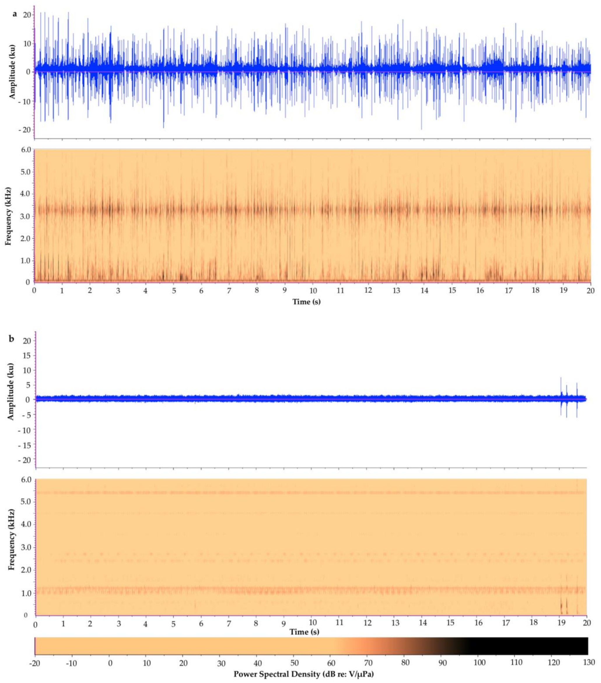
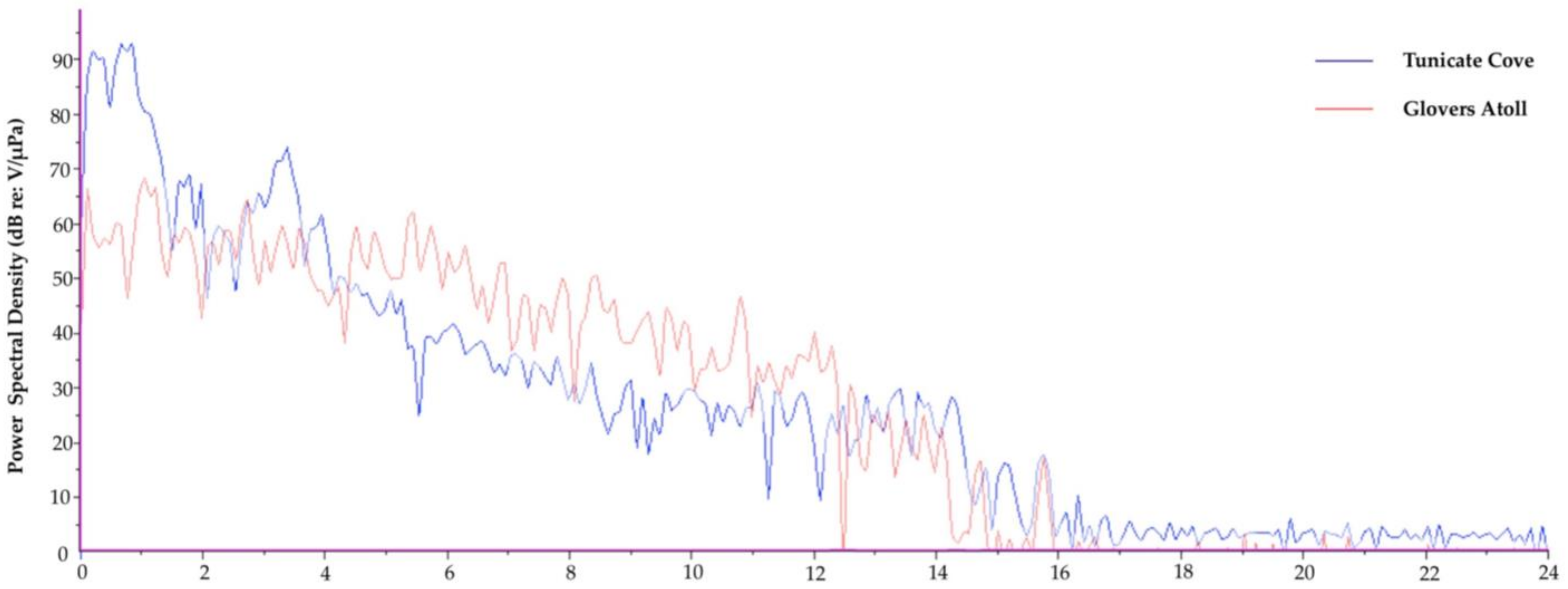
To demonstrate one approach, we show the following case study contrasting the soundscapes of two different marine habitats in Belize. The first recording is from a relatively quiet, sandy/mangrove habitat at Glovers Atoll; see Randall et al., [89] for a description of the study site. The other is from an acoustically complex, high biodiverse coral reef at Tunicate Cove; see Lindseth, [55] for a description of this habitat and recording methods. Each recording was visually and audibly inspected and cut to a 20-s clip that had minimal anthropogenic noise. Each 20-s clip was then analyzed in Raven Pro 1.4; see supplementary material for full details on the methods used to analyze the two recordings. The preliminary analyses of the 20-s clips from each recording display an acoustic difference between both the waveforms and spectrograms of the two different ecosystems (Figure 2 and Figure 3). Spatial variation between the two habitats (two-way analysis of variance (ANOVA) followed by a t test) was calculated. They revealed a statistical spatial variation between Tunicate Cove and Glovers Atoll for all of the parameters tested (n = 40, p < 0.0001) except for peak frequency (n = 40, F(1,38) = 0.32, p > 0.05). The more acoustically complex site with higher biodiversity (Tunicate Cove) had higher average (n = 40, F(1,38) = 1301.7, p < 0.0001) and peak PSD (n = 40, F(1,38) = 495.6, p < 0.0001), RMS amplitude (n = 40, F(1,38) = 765.4, p < 0.0001), and energy (n = 40, F(1,38) = 1309.9, p < 0.0001). However, both average entropy (n = 40, F(1,38) = 1524.2, p < 0.0001) and aggregate entropy (n = 40, F(1,38) = 324.4, p < 0.0001) were higher at Glovers Atoll, which is the sandy/mangrove habitat. It is important to note that in the very quiet recording of the sand habitat at Glovers Atoll, the camera’s operation noise can be heard, and it is seen in the spectrogram as a dark band at about 1.1 kHz to 1.2 kHz (see Kovitvongsa and Lobel, [90] for discussion of camera noise issues in acoustic recordings). These results from this preliminary case study are an example of how these two habitats can be acoustically differentiated. Table 4 itemizes recommended metrics and indices that can be reported when generally characterizing the soundscape of an area of study. It is recommended that future papers provide the same quantitative acoustic measurements, so that it will eventually be possible to directly compare results among studies and begin answering larger-scale questions on acoustic spatial and temporal variation.
7. Discussion
As an emerging scientific topic, soundscape ecology has advanced greatly in recent years with the number of scientific publications increasing mainly within the past 10 years (Figure 1). However, there is still a great deal that is unknown about how best to quantify acoustic signals and quantitatively compare data, especially among studies. Across dozens of studies from the past 10–15 years, most researchers recognize a handful of recommendations as logical next steps; these are detailed below. As many of these limitations and issues are solved, soundscape monitoring may offer a viable method for some wide-scale applications such as monitoring the health of remote habitats and documenting fish spawning activities.
In order to accurately describe the biodiversity of any habitat through acoustics and monitor the impacts of anthropogenic noise, the detection and documentation of fish sounds is key [3,11,38,46,58,59,61]. Fully understanding the hearing sensitivities of soniferous fishes is also important to understanding fishes’ communication in the context of their soundscape [21,47,52,74,81,91,92]. Currently, the acoustic signatures of marine mammals [67,93] and over 100 fish species have been well described [26,31,57,59,70,93,94,95,96,97]. The current best practice requires the use of hydrophones coupled with video recordings of the target species in order to confirm that a sound matches with an individual fish behavior [90,98]. However, the use of video to capture the calling fish is not always practical in the field due to limitations such as poor water visibility. It may be necessary to couple field and lab studies to definitively describe a species call. As the acoustic signatures of more species are better defined by clear recordings, the automatic detection features in bioacoustics software can be more finely tuned. The automatic detection of biological sounds will allow for simpler and faster analysis of large acoustic data files, which is needed to handle long-duration field recordings.
Directional hydrophones are useful in determining the source of a sound [43,99,100]. However, most studies currently use omnidirectional hydrophones, which are capable of picking up sounds from any direction. Terrestrial studies have used groups of directional microphones when examining population density, individual abundance, and locating and tracking animal movements [99]. These methods of localizing sources of sounds reduces the number of differences detected in recordings and allows for more accurate counts of individual sound producers [71,99,101]. A number of recent studies generalize entire acoustic habitats from single-point recordings [3,17,18,21,22,38,43,46,54,56]. The question is whether such limited spatial sampling is adequate. Perhaps multiple hydrophones in geographically distributed arrays would better ground truth patterns and aid in determining whether single-point recordings give an accurate representation of a broader area soundscape [57].
An integral part of any emerging field is to establish a common framework so that data are comparable among studies. In acoustics, this includes the standardization of the sampling/recording methods, metrics, and indices that are used in data analysis, visualization tools, sensor calibration, and ground truth current methods [1,23,38,54,57,58,61,65,68,99,102,103,104]. As more studies set long-term recording goals of several months or more, along with limitations of battery life and memory storage, studies are required to forego continuous recording. These same sampling schemes must not lose a significant amount of soundscape information. This issue was explored in tropical forests with the aim of determining how much acoustic information is lost as the gap in recording time increases [105]. Although the findings suggest that each location and soundscape may require a specialized recording schedule, overall, the loss of important information increases significantly with the gap between recording times [105]. These findings suggest that the best data comes from using a more intense recording regime.
One future application for soundscape ecology is the use of long-term recordings to monitor the health of an ecosystem. However, more long-term studies that explore the link between the health of an ecosystem and the corresponding soundscape parameters are needed [20,23,42]. A handful of studies have begun to explore the acoustic differences between a healthy habitat (i.e., forests, seagrass beds, coral reefs, etc.) to ones that have been degraded [19,23,44]. These studies have found suggestive differences in the acoustic signatures of healthy versus degraded habitats, but such differences may just as likely be based upon the variation in biological communities. The playback of healthy coral reef habitat sounds also results in greater attraction by the settlement stages of coral, mollusk, and coral reef fish larvae, which are migrating from offshore [5,6,7,8,11,106].
8. Conclusions
Underwater soundscapes and long-term PAM both have incredible potential in the fields of ecology, behavior, evolution, and conservation biology. Coupled with other conventional underwater survey methods and established physical oceanographic meters, PAM can be used to gain a more accurate understanding of the health, biodiversity, and structure of underwater habitats. Acoustics may enable researchers to monitor several different species simultaneously, which offers an integrative look at different habitats within and between ecosystems [99]. PAM provides a new technology to monitor remote underwater habitats over long durations. However, when beginning at any new site, it will probably be necessary to use synchronous audio and video recordings alongside conventional visual surveys in order to get an accurate assessment of a particular underwater habitat and verify sound-producing species.
Supplementary Materials
The following are available online at https://www.mdpi.com/2410-3888/3/3/36/s1, Methods S1: Methods for habitat comparison between Tunicate Cove and Glovers Atoll, Belize, Video S1: Tunicate Cove 20 s clip, Video S2: Glovers Atoll 20 s clip.
Author Contributions
This article is based on a Master’s thesis by A.V.L.; Project Conceptualization, A.V.L. and P.S.L.; Methodology, A.V.L. and P.S.L.; Original field recordings, P.S.L.; Software, A.V.L.; Writing-Original Draft Preparation, A.V.L.; Writing-Review & Editing, A.V.L. and P.S.L.
Funding
This research received no external funding.
Acknowledgments
We thank Ingrid Kaatz and Aaron Rice for long time discussions on these topics and reviewers for helpful comments.
Conflicts of Interest
The authors declare no conflict of interest.
References
- Pijanowski, B.C.; Villanueva-Rivera, L.J.; Dumyahn, S.L.; Farina, A.; Krause, B.L.; Napoletano, B.M.; Gage, S.H.; Pieretti, N. Soundscape ecology: The science of sound in the landscape. BioScience 2011, 61, 203–216. [Google Scholar] [CrossRef]
- Schafer, R.M. The Tuning of the World; Alfred A. Knopf: New York, NY, USA, 1977; ISBN 0-394-40966-3. [Google Scholar]
- Staaterman, E.; Rice, A.N.; Mann, D.A.; Paris, C.B. Soundscapes from a tropical Eastern Pacific reef and a Caribbean Sea reef. Coral Reefs 2013, 32, 553–557. [Google Scholar] [CrossRef]
- Lobel, P.S. The “choral reef”: The ecology of underwater sounds. In Proceedings of the 2013 AAUS/ESDP Curaçao Joint International Scientific Diving Symposium, Dauphin Island, AL, USA, 24–27 October 2013; pp. 179–185. [Google Scholar]
- Jolivet, A.; Tremblay, R.; Olivier, F.; Gervaise, C.; Sonier, R.; Genard, B.; Chauvaud, L. Validation of trophic and anthropic underwater noise as settlement trigger in blue mussels. Sci. Rep. 2016, 6, 1–8. [Google Scholar] [CrossRef] [PubMed] [Green Version]
- Lillis, A.; Bohnenstiehl, D.; Peters, J.W.; Eggleston, D. Variation in habitat soundscape characteristics influences settlement of a reef-building coral. PeerJ 2016, 4. [Google Scholar] [CrossRef] [PubMed] [Green Version]
- Lillis, A.; Eggleston, D.B.; Bohnenstiehl, D.R. Oyster larvae settle in response to habitat-associated underwater sounds. PLoS ONE 2013, 8, 79337. [Google Scholar] [CrossRef] [PubMed]
- Lillis, A.; Eggleston, D.B.; Bohnenstiehl, D.R. Soundscape variation from a larval perspective: The case for habitat-associated sound as a settlement cue for weakly swimming estuarine larvae. Mar. Ecol. Prog. Ser. 2014, 509, 57–70. [Google Scholar] [CrossRef]
- Lobel, P.S. Scuba bubble noise and fish behavior: A rationale for silent diving technology. In Proceedings of the American Academy of Underwater Sciences; University of Connecticut: Storrs, CT, USA, 2005; pp. 49–59. [Google Scholar]
- Lobel, P.S. Underwater acoustic ecology: Boat noises and fish behavior. In Proceedings of the American Academy of Underwater Sciences 28th Symposium, Atlanta, GA, USA, 13–14 March 2009; Pollock, N.W., Ed.; AAUS: Dauphin Island, AL, USA, 2009; pp. 31–42. [Google Scholar]
- Vermeij, M.J.A.; Marhaver, K.L.; Huijbers, C.M.; Nagelkerken, I.; Simpson, S.D. Coral larvae move toward reef sounds. PLoS ONE 2010, 5, 10660. [Google Scholar] [CrossRef] [PubMed] [Green Version]
- Fish, M.P.; Mowbray, W.H. Sounds of Western North Atlantic Fishes. A Reference File of Biological Underwater Sounds; Rhode Island Univ Kingston Narragansett Marine Lab: Kingston, RI, USA, 1970. [Google Scholar]
- Myrberg, A.; Spanier, E.; Ha, S.J. Temporal patterning in acoustical communication. In Contrasts in Behavior; Wiley: New York, NY, USA, 1978; pp. 137–179. [Google Scholar]
- Tavolga, W.N.; Lanyon, W.E. Animal Sounds and Communication; American Institute of Biological Sciences: Washington, DC, USA, 1960. [Google Scholar]
- Winn, H. The biological significance of fish sounds. Mar. Bio-Acoust. 1964, 2, 213–231. [Google Scholar]
- Fine, M.L.; Winn, H.; Olla, B.L. Communication in fishes. In How Animals Communicate; Sebeok, T.A., Ed.; Indiana University Press: Bloomington, IN, USA, 1977; pp. 472–518. [Google Scholar]
- Au, W.W.L.; Richlen, M.; Lammers, M.O. Soundscape of a nearshore coral reef near an urban center. Adv. Exp. Med. Biol. 2012, 730, 345–351. [Google Scholar] [CrossRef] [PubMed]
- Bertucci, F.; Parmentier, E.; Berten, L.; Brooker, R.M.; Lecchini, D. Temporal and spatial comparisons of underwater sound signatures of different reef habitats in Moorea Island, French Polynesia. PLoS ONE 2015, 10, 135733. [Google Scholar] [CrossRef] [PubMed]
- Butler, J.; Stanley, J.A.; Butler, M.J. Underwater soundscapes in near-shore tropical habitats and the effects of environmental degradation and habitat restoration. J. Exp. Mar. Biol. Ecol. 2016, 479, 89–96. [Google Scholar] [CrossRef]
- Lammers, M.O.; Brainard, R.E.; Au, W.W.L.; Mooney, T.A.; Wong, K.B. An ecological acoustic recorder (EAR) for long-term monitoring of biological and anthropogenic sounds on coral reefs and other marine habitats. J. Acoust. Soc. Am. 2008, 123, 1720–1728. [Google Scholar] [CrossRef] [PubMed]
- Rossi, T.; Connell, S.D.; Nagelkerken, I. The sounds of silence: Regime shifts impoverish marine soundscapes. Landsc. Ecol. 2017, 32, 239–248. [Google Scholar] [CrossRef]
- Staaterman, E.; Ogburn, M.B.; Altieri, A.H.; Brandl, S.J.; Whippo, R.; Seemann, J.; Goodison, M.; Duffy, J.E. Bioacoustic measurements complement visual biodiversity surveys: Preliminary evidence from four shallow marine habitats. Mar. Ecol. Prog. Ser. 2017, 575, 207–215. [Google Scholar] [CrossRef]
- Sueur, J.; Pavoine, S.; Hamerlynck, O.; Duvail, S. Rapid acoustic survey for biodiversity appraisal. PLoS ONE 2008, 3, 4065. [Google Scholar] [CrossRef] [PubMed]
- Lobel, P.S. Fish bioacoustics and behavior: Passive acoustic detection and the application of a closed-circuit rebreather for field study. Mar. Technol. Soc. J. 2001, 35, 19–28. [Google Scholar] [CrossRef]
- Lobel, P.S. Sounds produced by spawning fishes. Environ. Biol. Fish. 1992, 33, 351–358. [Google Scholar] [CrossRef]
- Lobel, P.S.; Mann, D.A. Spawning sounds of the damselfish, Dascyllus albisella (Pomacentridae), and relationship to male size. Bioacoustics 1995, 6, 187–198. [Google Scholar] [CrossRef]
- Mann, D.A.; Lobel, P.S. Passive acoustic detection of sounds produced by the Damselfish, Dascyllus albisella (Pomacentridae). Bioacoustics 1995, 6, 199–213. [Google Scholar] [CrossRef]
- Rountree, R.A.; Gilmore, R.G.; Goudey, C.A.; Hawkins, A.D.; Luczkovich, J.J.; Mann, D.A. Listening to fish: Applications of passive acoustics to fisheries science. Fisheries 2006, 31, 433–446. [Google Scholar] [CrossRef]
- Luczkovich, J.J.; Pullinger, R.C.; Johnson, S.E.; Sprague, M.W. Identifying sciaenid critical spawning habitats by the use of passive acoustics. Trans. Am. Fish. Soc. 2008, 137, 576–605. [Google Scholar] [CrossRef]
- Rowell, T.J.; Demer, D.A.; Aburto-Oropeza, O.; Cota-Nieto, J.J.; Hyde, J.R.; Erisman, B.E. Estimating fish abundance at spawning aggregations from courtship sound levels. Sci. Rep. 2017, 7. [Google Scholar] [CrossRef] [PubMed] [Green Version]
- Lobel, P.S.; Rice, A.N.; Kaatz, I.M. Acoustic behavior of coral reef fishes. In Reproduction and Sexuality in Marine Fishes: Patterns and Processes; University of California Press: Berkeley, CA, USA, 2010; pp. 307–347. ISBN 978-0-520-26433-5. [Google Scholar]
- Bass, A.H.; McKibben, J.R. Neural mechanisms and behaviors for acoustic communication in teleost fish. Prog. Neurobiol. 2003, 69, 1–26. [Google Scholar] [CrossRef]
- Radford, A.N.; Kerridge, E.; Simpson, S.D. Acoustic communication in a noisy world: Can fish compete with anthropogenic noise? Behav. Ecol. 2014, 25, 1022–1030. [Google Scholar] [CrossRef]
- Fine, M.L.; Parmentier, E. Mechanisms of fish sound production. In Sound Communication in Fishes; Ladich, F., Ed.; Springer-Verlag: Berlin/Heidelberg, Germany; Vienna, Austria, 2015; Volume 4, pp. 77–126. ISBN 978-3-7091-1845-0. [Google Scholar]
- Lobel, P.S.; Lobel, L.K. Stalking spawning fishes. In Proceedings of the 2013 AAUS/ESDP Curaçao Joint International Scientific Diving Symposium, Dauphin Island, AL, USA, 24–27 October 2013; pp. 179–185. [Google Scholar]
- Felisberto, P.; Rodríguez, O.; Santos, P.; Zabel, F.; Jesus, S.M. Using passive acoustics for monitoring seagrass beds. In Proceedings of the Oceans 2016 MTS/IEEE Monterey, Monterey, CA, USA, 19–23 September 2016. [Google Scholar] [CrossRef]
- Radford, C.A.; Jeffs, A.G.; Tindle, C.T.; Montgomery, J.C.; Montgomery, J.C. Temporal patterns in ambient noise of biological origin from a shallow water temperate reef. Oecologia 2008, 156, 921–929. [Google Scholar] [CrossRef] [PubMed]
- Staaterman, E.; Paris, C.B.; DeFerrari, H.A.; Mann, D.A.; Rice, A.N.; D’Alessandro, E.K. Celestial patterns in marine soundscapes. Mar. Ecol. Prog. Ser. 2014, 508, 17–32. [Google Scholar] [CrossRef]
- Locascio, J.V.; Mann, D.A. Diel periodicity of fish sound production in Charlotte Harbor, Florida. Trans. Am. Fish. Soc. 2008, 137, 606–615. [Google Scholar] [CrossRef]
- Wenz, G.M. Acoustic Ambient Noise in the Ocean: Spectra and Sources. J. Acoust. Soc. Am. 1962, 34, 1936–1956. [Google Scholar] [CrossRef]
- University of Rhode Island What Are Common Underwater Sounds? Available online: https://dosits.org/science/sounds-in-the-sea/what-are-common-underwater-sounds/ (accessed on 1 September 2018).
- Pieretti, N.; Farina, A.; Morri, D. A new methodology to infer the singing activity of an avian community: The Acoustic Complexity Index (ACI). Ecol. Indic. 2011, 11, 868–873. [Google Scholar] [CrossRef]
- Pieretti, N.; Lo Martire, M.; Farina, A.; Danovaro, R. Marine soundscape as an additional biodiversity monitoring tool: A case study from the Adriatic Sea (Mediterranean Sea). Ecol. Indic. 2017, 83, 13–20. [Google Scholar] [CrossRef]
- Piercy, J.J.B.; Codling, E.A.; Hill, A.J.; Smith, D.J.; Simpson, S.D. Habitat quality affects sound production and likely distance of detection on coral reefs. Mar. Ecol. Prog. Ser. 2014, 516, 35–47. [Google Scholar] [CrossRef] [Green Version]
- Parmentier, E.; Berten, L.; Rigo, P.; Aubrun, F.; Nedelec, S.L.; Simpson, S.D.; Lecchini, D. The influence of various reef sounds on coral-fish larvae behaviour. J. Fish. Biol. 2015, 86, 1507–1518. [Google Scholar] [CrossRef] [PubMed]
- Radford, C.A.; Stanley, J.A.; Simpson, S.D.; Jeffs, A.G. Juvenile coral reef fish use sound to locate habitats. Coral Reefs 2011, 30, 295–305. [Google Scholar] [CrossRef]
- Barth, P.; Berenshtein, I.; Besson, M.; Roux, N.; Parmentier, E.; Banaigs, B.; Lecchini, D. From the ocean to a reef habitat: How do the larvae of coral reef fishes find their way home? A state of art on the latest advances. Vie et Milieu 2015, 65, 91–100. [Google Scholar]
- Simpson, S.D.; Meekan, M.G.; Jeffs, A.; Montgomery, J.C.; McCauley, R.D. Settlement-stage coral reef fish prefer the higher-frequency invertebrate-generated audible component of reef noise. Anim. Behav. 2008, 75, 1861–1868. [Google Scholar] [CrossRef]
- Simpson, S.D.; Meekan, M.G.; Larsen, N.J.; McCauley, R.D.; Jeffs, A. Behavioral plasticity in larval reef fish: Orientation is influenced by recent acoustic experiences. Behav. Ecol. 2010, 21, 1098–1105. [Google Scholar] [CrossRef]
- Heenan, A.; Simpson, S.D.; Braithwaite, V.A. Testing the Generality of Acoustic Cue Use at Settlement in Larval Coral Reef Fish. 6. Available online: https://www.researchgate.net/profile/Stephen_Simpson5/publication/266447888_Testing_the_generality_of_acoustic_cue_use_at_settlement_in_larval_coral_reef_fish/links/54b6494d0cf26833efd36db8/Testing-the-generality-of-acoustic-cue-use-at-settlement-in-larval-coral-reef-fish.pdf. (accessed on 1 September 2018).
- Lecchini, D.; Shima, J.; Banaigs, B.; Galzin, R. Larval sensory abilities and mechanisms of habitat selection of a coral reef fish during settlement. Oecologia 2005, 143, 326–334. [Google Scholar] [CrossRef] [PubMed]
- Mann, D.; Casper, B.; Boyle, K.; Tricas, T. On the attraction of larval fishes to reef sounds. Mar. Ecol. Prog. Ser. 2007, 338, 307–310. [Google Scholar] [CrossRef] [Green Version]
- Curtis, K.R.; Howe, B.M.; Mercer, J.A.; Curtis, K.R.; Howe, B.M.; Mercer, J.A. Low-frequency ambient sound in the North Pacific: Long time series observations. J. Acoust. Soc. Am. 1999, 106, 3189–3200. [Google Scholar] [CrossRef]
- Haxel, J.H.; Dziak, R.P.; Matsumoto, H. Observations of shallow water marine ambient sound: The low frequency underwater soundscape of the central Oregon coast. J. Acoust. Soc. Am. 2013, 133, 2586–2596. [Google Scholar] [CrossRef] [PubMed]
- Lindseth, A.V. Determining temporal recording schemes for underwater acoustic monitoring studies. Master’s Thesis, Boston University, Boston, MA, USA, 2019; p. 42. [Google Scholar]
- Heenehan, H.L.; Van Parijs, S.M.; Bejder, L.; Tyne, J.A.; Southall, B.L.; Southall, H.; Johnston, D.W. Natural and anthropogenic events influence the soundscapes of four bays on Hawaii Island. Mar. Pollut. Bull. 2017, 124, 9–20. [Google Scholar] [CrossRef] [PubMed]
- Rowell, T.J.; Schärer, M.T.; Appeldoorn, R.S.; Nemeth, M.I.; Mann, D.A.; Rivera, J.A. Sound production as an indicator of red hind density at a spawning aggregation. Mar. Ecol. Prog. Ser. 2012, 462, 241–250. [Google Scholar] [CrossRef] [Green Version]
- Wall, C.C.; Mann, D.A.; Lembke, C.; Taylor, C.; He, R.; Kellison, T. Mapping the soundscape off the southeastern USA by using passive acoustic glider technology. Mar. Coast. Fish. 2017, 9, 23–37. [Google Scholar] [CrossRef]
- Locascio, J.V.; Burton, M.L. A passive acoustic survey of fish sound production at Riley’s Hump within Tortugas South Ecological Reserve: Implications regarding spawning and habitat use. Fish. Bull. 2015, 114, 103–116. [Google Scholar] [CrossRef]
- Depraetere, M.; Pavoine, S.; Jiguet, F.; Gasc, A.; Duvail, S.; Sueur, J. Monitoring animal diversity using acoustic indices: Implementation in a temperate woodland. Ecol. Indic. 2012, 13, 46–54. [Google Scholar] [CrossRef]
- Kaplan, M.B.; Mooney, T.A.; Partan, J.; Solow, A.R. Coral reef species assemblages are associated with ambient soundscapes. Mar. Ecol. Prog. Ser. 2015, 533, 93–107. [Google Scholar] [CrossRef] [Green Version]
- Benoit-Bird, K.J.; Au, W.W.L.; Brainard, R.E.; Lammers, M.O. Diel horizontal migration of the Hawaiian mesopelagic boundary community observed acoustically. Mar. Ecol. Prog. Ser. 2001, 217, 1–14. [Google Scholar] [CrossRef] [Green Version]
- Stanley, J.A.; Van Parijs, S.M.; Hatch, L.T. Underwater sound from vessel traffic reduces the effective communication range in Atlantic cod and haddock. Sci. Rep. 2017, 7, 1–12. [Google Scholar] [CrossRef]
- Wiggins, S.M.; Hall, J.M.; Thayre, B.J.; Hildebrand, J.A. Gulf of Mexico low-frequency ocean soundscape impacted by airguns. J. Acoust. Soc. Am. 2016, 140, 176–183. [Google Scholar] [CrossRef] [PubMed] [Green Version]
- Parks, S.E.; Miksis-Olds, J.L.; Denes, S.L. Assessing marine ecosystem acoustic diversity across ocean basins. Ecol. Inf. 2014, 21, 81–88. [Google Scholar] [CrossRef]
- Brown, M.G.; Godin, O.A.; Zang, X.; Ball, J.S.; Zabotin, N.A.; Zabotina, L.Y.; Williams, N.J. Ocean acoustic remote sensing using ambient noise: Results from the Florida Straits. Geophy. J. Int. 2016, 206, 574–589. [Google Scholar] [CrossRef]
- Gavrilov, A.N.; Parsons, M.J.G. A Matlab tool for the characterisation of recorded underwater sound (CHORUS). Acoust. Aust. 2014, 42, 190–196. [Google Scholar]
- Merchant, N.D.; Fristrup, K.M.; Johnson, M.P.; Tyack, P.L.; Witt, M.J.; Blondel, P.; Parks, S.E. Measuring acoustic habitats. Methods Ecol. Evol. 2015, 6, 257–265. [Google Scholar] [CrossRef] [PubMed] [Green Version]
- Fisher-pool, P.I.; Lammers, M.O.; Gove, J.; Wong, K.B. Does primary productivity turn up the volume? Exploring the relationship between chlorophyll a and the soundscape of coral reefs in the Pacific. Adv. Exp. Med. Biol. 2016, 875, 289–293. [Google Scholar] [CrossRef] [PubMed]
- Morisaka, T.; Shinohara, M.; Nakahara, F.; Akamatsu, T. Effects of ambient noise on the whistles of Indo-Pacific bottlenose dolphin populations. J. Mammal. 2005, 86, 541–546. [Google Scholar] [CrossRef]
- McWilliam, J.N.; Hawkins, A.D. A comparison of inshore marine soundscapes. J. Exp. Mar. Biol. Ecol. 2013, 446, 166–176. [Google Scholar] [CrossRef]
- Wang, H.; Elson, J.; Girod, L.; Estrin, D.; Yao, K. Target classification and localization in habitat monitoring. ICASSP IEEE Int. Conf. Acoust. Speech Signal. Process. 2003, 4, 844–847. [Google Scholar] [CrossRef]
- Porter, M.; Henderson, L. Global ocean soundscapes. Proc. Meet. Acoust. 2013, 19, 1–6. [Google Scholar] [CrossRef]
- Staaterman, E.; Paris, C.B.; Kough, A.S. First evidence of fish larvae producing sounds. Biol. Lett. 2014, 10, 20140643. [Google Scholar] [CrossRef] [PubMed]
- Sueur, J.; Farina, A.; Gasc, A.; Pieretti, N.; Pavoine, S. Acoustic indices for biodiversity assessment and landscape investigation. Acta Acust. United Acust. 2014, 100, 772–781. [Google Scholar] [CrossRef]
- Bolgan, M.; Amorim, M.C.P.; Fonseca, P.J.; Di Iorio, L.; Parmentier, E. Acoustic complexity of vocal fish communities: A field and controlled validation. Sci. Rep. 2018, 8. [Google Scholar] [CrossRef] [PubMed]
- Rice, A.N.; Soldevilla, M.S.; Quinlan, J.A. Nocturnal patterns in fish chorusing off the coasts of Georgia and eastern Florida. Bull. Mar. Sci. 2017, 93, 455–474. [Google Scholar] [CrossRef]
- Towsey, M.; Wimmer, J.; Williamson, I.; Roe, P. The use of acoustic indices to determine avian species richness in audio-recordings of the environment. Ecol. Inf. 2014, 21, 110–119. [Google Scholar] [CrossRef]
- Towsey, M.; Zhang, L.; Cottman-Fields, M.; Wimmer, J.; Zhang, J.; Roe, P. Visualization of long-duration acoustic recordings of the environment. Proced. Comput. Sci. 2014, 29, 703–712. [Google Scholar] [CrossRef]
- Harris, S.A.; Shears, N.T.; Radford, C.A. Ecoacoustic indices as proxies for biodiversity on temperate reefs. Methods Ecol. Evol. 2016, 7, 713–724. [Google Scholar] [CrossRef]
- Villanueva-Rivera, L.J.; Pijanowski, B.C.; Doucette, J.; Pekin, B. A primer of acoustic analysis for landscape ecologists. Landsc. Ecol. 2011, 26, 1233–1246. [Google Scholar] [CrossRef]
- Sueur, J.; Aubin, T.; Simonis, C. Sound analysis and synthesis with the package Seewave. Bioacoustics 2008, 18, 213–226. [Google Scholar] [CrossRef]
- Bertucci, F.; Parmentier, E.; Berthe, C.; Besson, M.; Hawkins, A.D.; Aubin, T.; Lecchini, D. Snapshot recordings provide a first description of the acoustic signatures of deeper habitats adjacent to coral reefs of Moorea. PeerJ 2017, 5, e4019. [Google Scholar] [CrossRef] [PubMed]
- Erbe, C.; Verma, A.; McCauley, R.; Gavrilov, A.; Parnum, I. The marine soundscape of the Perth Canyon. Prog. Oceanogr. 2015, 137, 38–51. [Google Scholar] [CrossRef]
- Felisberto, P.; Rodriguez, O.; Santos, P.; Zabel, F.; Jesus, S. Variability of the ambient noise in a seagrass bed. In Proceedings of the IEEE 2014 Oceans, St. John’s, NL, USA, 14–19 September 2014; pp. 1–6. [Google Scholar]
- Radford, C.; Stanley, J.; Tindle, C.; Montgomery, J.; Jeffs, A. Localised coastal habitats have distinct underwater sound signatures. Mar. Ecol. Prog. Ser. 2010, 401, 21–29. [Google Scholar] [CrossRef] [Green Version]
- Radford, C.; Stanley, J.; Jeffs, A. Adjacent coral reef habitats produce different underwater sound signatures. Mar. Ecol. Prog. Ser. 2014, 505, 19–28. [Google Scholar] [CrossRef]
- Roth, E.H.; Hildebrand, J.A.; Wiggins, S.M.; Ross, D. Underwater ambient noise on the Chukchi Sea continental slope from 2006–2009. J. Acoust. Soc. Am. 2012, 131, 104–110. [Google Scholar] [CrossRef] [PubMed]
- Randall, J.E.; Lobel, P.S.; Kennedy, C.W. Comparative ecology of the gobies Nes longus and Ctenogobius saepepallens, both symbiotic with the snapping shrimp Alpheus floridanus. Environ. Biol. Fish. 2005, 74, 119–127. [Google Scholar] [CrossRef]
- Kovitvongsa, K.E.; Lobel, P.S. Convenient fish acoustic data collection in the digital age. In Proceedings of the American Academy of Underwater Sciences 28th Symposium, Atlanta, GA, USA, 13–14 March 2009; Pollock, N.W., Ed.; AAUS: Dauphin Island, AL, USA, 2009; pp. 43–57. [Google Scholar]
- Erbe, C. Underwater passive acoustic monitoring & noise impacts on marine fauna-A workshop report. Acoust. Aust. 2013, 41, 211–217. [Google Scholar]
- Giard, J.L.; Vigness-Raposa, K.J.; Frankel, A.S.; Ellison, W.T. Visualization of spatially explicit acoustic layers in an underwater soundscape. In Proceedings of Meetings on Acoustics; Acoustical Society of America: Dublin, Ireland, 2016; Volume 27. [Google Scholar]
- Mann, D.A.; Lobel, P.S. Propagation of damselfish (Pomacentridae) courtship sounds. J. Acoust. Soc. Am. 1997, 101, 3783–3791. [Google Scholar] [CrossRef]
- Mosharo, K.K.; Lobel, P.S. Acoustic signals of two toadfishes from Belize: Sanopus astrifer and Batrachoides gilberti (Batrachoididae). Environ. Biol. Fish. 2012, 94, 623–638. [Google Scholar] [CrossRef]
- Ripley, J.L.; Lobel, P.S. Correlation of acoustic and visual signals in the cichlid fish, Tramitichromis intermedius. Environ. Biol. Fish. 2004, 71, 389–394. [Google Scholar] [CrossRef]
- Tricas, T.; Boyle, K. Acoustic behaviors in Hawaiian coral reef fish communities. Mar. Ecol. Prog. Ser. 2014, 511, 1–16. [Google Scholar] [CrossRef] [Green Version]
- Tricas, T.C.; Webb, J.F. Acoustic communication in butterflyfishes: Anatomical novelties, physiology, evolution, and behavioral ecology. Adv. Exp. Med. Biol. 2016, 877, 57–92. [Google Scholar]
- Lobel, P. Diversity of fish courtship and spawning sounds and application for monitoring reproduction. J. Acoust. Soc. Am. 2002, 112, 2201–2202. [Google Scholar] [CrossRef]
- Blumstein, D.T.; Mennill, D.J.; Clemins, P.; Girod, L.; Yao, K.; Patricelli, G.; Deppe, J.L.; Krakauer, A.H.; Clark, C.; Cortopassi, K.A.; et al. Acoustic monitoring in terrestrial environments using microphone arrays: Applications, technological considerations and prospectus. J. Appl. Ecol. 2011, 48, 758–767. [Google Scholar] [CrossRef]
- Dushaw, B.; Au, W.W.L.; Beszczynska-Moller, A.; Brainard, R.E.; Cornuelle, B.D.; Duda, T.F.; Dzieciuch, M.A.; Fahrbach, E.; Forbes, A.; Freitag, L.; et al. A Global Ocean Acoustic Observing Network. 2009. Available online: https://www.researchgate.net/publication/263031402_A_Global_Ocean_Acoustic_Observing_Network (accessed on 1 September 2018).
- Frommolt, K.H.; Tauchert, K.H. Applying bioacoustic methods for long-term monitoring of a nocturnal wetland bird. Ecol. Inf. 2014, 21, 4–12. [Google Scholar] [CrossRef]
- Brainard, R.; Bainbridge, S.; Brinkman, R.; Eakin, C.M.; Field, M.; Gattuso, P.; Gledhill, D.; Gramer, L.; Green, A.; Hendee, J.; et al. An International Network of Coral Reef Ecosystem Observing Systems (I-CREOS). 2009. Available online: http://www.obs-vlfr.fr/~gattuso/publications_PDF/Brainard_etal_2009.pdf (accessed on 1 September 2018).
- Hatch, L.T.; Wahle, C.M.; Gedamke, J.; Harrison, J.; Laws, B.; Moore, S.E.; Stadler, J.H.; Van Parijs, S.M. Can you hear me here? Managing acoustic habitat in US waters. Endanger. Species Res. 2016, 30, 171–186. [Google Scholar] [CrossRef] [Green Version]
- Og̃uz, H.N. A theoretical study of low-frequency oceanic ambient noise. J. Acoust. Soc. Am. 1994, 95, 1895. [Google Scholar] [CrossRef]
- Pieretti, N.; Duarte, M.H.L.; Sousa-Lima, R.S.; Rodrigues, M.; Young, R.J.; Farina, A. Determining temporal sampling schemes for passive acoustic studies in different tropical ecosystems. Trop. Conserv. Sci. 2015, 8, 215–234. [Google Scholar] [CrossRef]
- Eggleston, D.B.; Lillis, A.; Bohnenstiehl, D.R. Soundscapes and larval settlement: Larval bivalve responses to habitat-associated underwater sounds. In The Effects of Noise on Aquatic Life II; Popper, A.N., Hawkins, A., Eds.; Advances in Experimental Medicine and Biology, Springer: Berlin, Germany, 2016; Volume 875, pp. 255–263. [Google Scholar]
Figure 1.
Number of “soundscape ecology” scientific papers published per year. Data derived by searching Google Scholar using only the keyword “soundscape ecology”, and does not reflect earlier works of describing underwater acoustics and marine animal sounds. The number above each bar is the number of publications for that year.
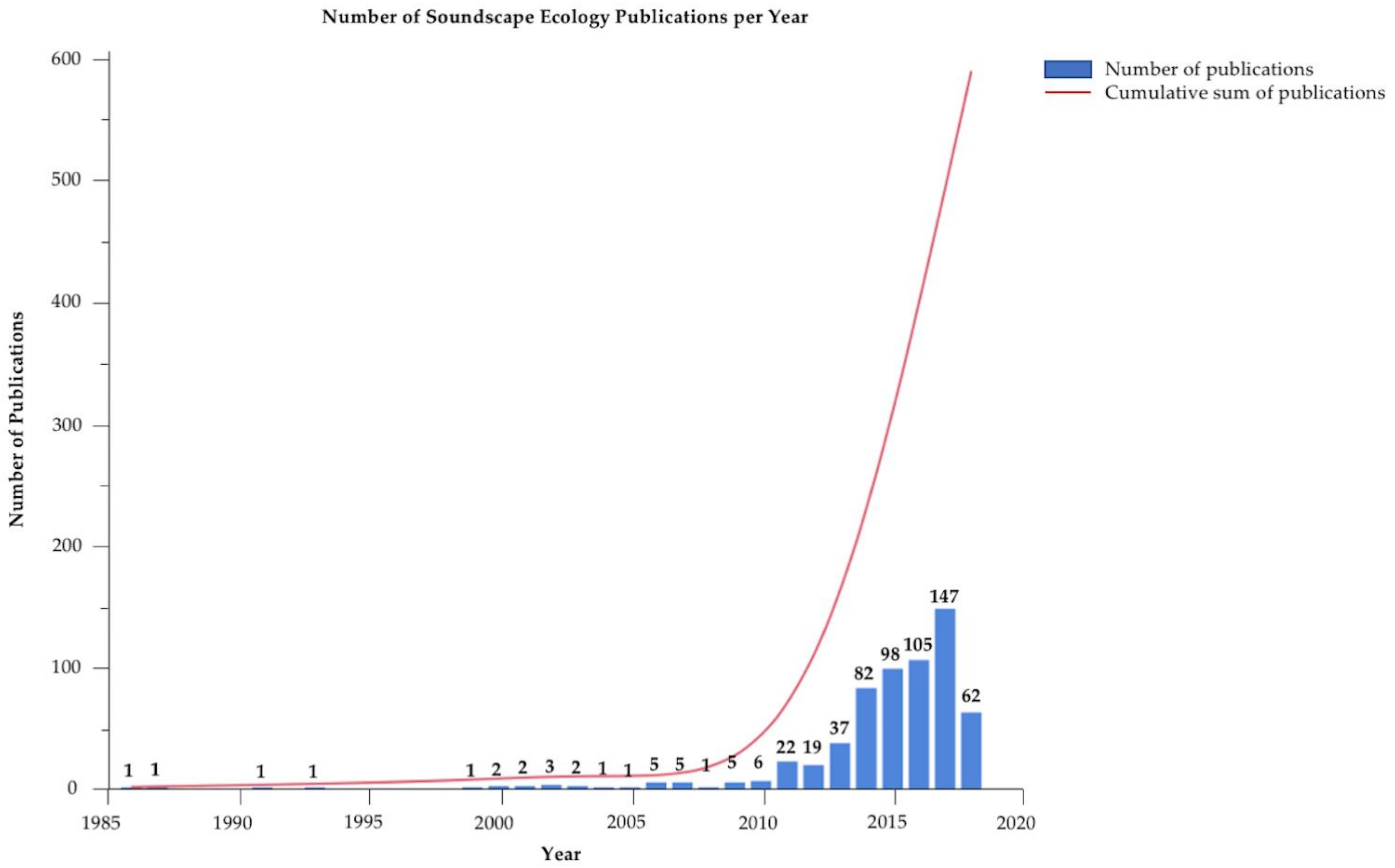
Figure 2.
Waveform and spectrogram of (a) a 20-s recording from Tunicate Cove, Belize, 1996 and (b) a 20-s recording from Glovers Atoll, Belize, 1999. Note: the dark band at around 1.1 kHz–1.2 kHz is from camera noise, which is evident in this overall very quiet recording. The bottom row is the color bar representing the power spectral density (in dB) values in the spectrograms.

Figure 3.
Dominant frequency plots comparing Tunicate Cove, Belize (blue) and Glovers Atoll, Belize (green).
Figure 3.
Dominant frequency plots comparing Tunicate Cove, Belize (blue) and Glovers Atoll, Belize (green).


Table 1.
Recording rates used in various underwater soundscape ecology and/or long-term passive acoustic monitoring (PAM) studies. GBR: Great Barrier Reef, US: United States.
Table 1.
Recording rates used in various underwater soundscape ecology and/or long-term passive acoustic monitoring (PAM) studies. GBR: Great Barrier Reef, US: United States.
| Recording Rate | Paper | Location |
|---|---|---|
| 30 s every 4 min | [56] | Hawaii, US |
| 12 s every 5 min | [38] | Florida Keys, US |
| 12 s every 5 min | [3] | Florida Keys, US; Panama |
| 20 s every 5 min | [57] | Puerto Rico; US Virgin Islands |
| 30 s every 5 min | [58] | Southeast USA waters |
| 10 s every 10 min | [59] | Florida Keys, US |
| 1 min every 10 min | [22] | Bocas del Toro, Panama |
| 2 min every 10 min | [6] | Curaçao |
| 30 s every 15 min | [20] | Oahu, Hawaii, US |
| 150 s every 15 min | [60] | France |
| 1 min every 20 min | [61] | St. John, US Virgin Islands |
| 10 min every 1 h | [46] | Lizard Island, GBR, Australia |
| 1 h every 3 h | [62] | Hawaii, US |
| Continuously for 24 h | [5] | Prince Edward Island, Canada |
| Continuously for 24 h | [22] | Bocas del Toro, Panama |
| Continuously for 48 h | [43] | Adriatic Sea, Italy |
Table 2.
Recording frequency rates used in various underwater soundscape ecology and/or long-term passive acoustic monitoring publications. NMS: National Marine Sanctuaries.
Table 2.
Recording frequency rates used in various underwater soundscape ecology and/or long-term passive acoustic monitoring publications. NMS: National Marine Sanctuaries.
| Recording Frequency Rate | Paper | Location |
|---|---|---|
| 2 kHz | [54] | Oregon, US |
| 2 kHz | [63] | Stellwagen Bank NMS, USA |
| 2 kHz | [64] | Gulf of Mexico |
| 20 kHz | [3] | Florida Keys, US; Panama |
| 44.1 kHz | [11] | Curaçao |
| 96 kHz | [6] | Curaçao |
| 96 kHz | [21] | Adelaide, South Australia, Australia |
| 250 kHz | [65] | Ascension Island; Diego Garcia Island; Wake Island |
Table 3.
Definitions, assumptions/limitations, and group of acoustic indices.
| Index | Definition | Assumption/Limitation | Group | Reference(s) |
|---|---|---|---|---|
| Acoustic Entropy (H) | Evenness/species richness of acoustic space | Combines spectral and temporal H | α | 1. [23] |
| 0 = pure tones; 1 = random noise; | 2. [22,60,61,65,78,79,80] | |||
| Geophony/anthrophony reduce reliability and produce false high values | ||||
| Acoustic Richness (AR) | Species richness of acoustic space | Combines temporal H and amplitude; | α | 1. [60] |
| = pure tones; 1 = random noise; | 2. [23,80] | |||
| More accurate than H in areas of lower diversity | ||||
| Acoustic Dissimilarity Index (D) | Dissimilarity between two communities | Compares two signals of same duration and frequency; | β | 1. [23] |
| 2. [60] | ||||
| 0 = similar sounds; 1 = distinct sounds | ||||
| increases with number of unshared chorus pairs | ||||
| Acoustic Complexity Index (ACI) | Degree of complexity | Sums absolute difference between two adjacent intensities; better for soundscapes of constant intensity; | α | 1. [42] |
| 2, [1,19,22,38,43,61,71,78,79,80] | ||||
| Reliability reduced if one dominant acoustic spp.; | ||||
| time-consuming calculations |
1. First mention of index 2. Other studies that have used that index.
Table 4.
Example of soundscape features from a healthy coral reef at Tunicate Cove and a shallow mangrove–sand habitat in Belize. Each mean and standard deviation (S.D.) were calculated from n = 20 1-s selections from a total 20-s sound clip.
Table 4.
Example of soundscape features from a healthy coral reef at Tunicate Cove and a shallow mangrove–sand habitat in Belize. Each mean and standard deviation (S.D.) were calculated from n = 20 1-s selections from a total 20-s sound clip.
| Tunicate Cove | Glovers Atoll Mangrove | |
|---|---|---|
| Acoustic Metric | Mean ± S.D. (Range) n = 20 | Mean ± S.D. (Range) n = 20 |
| Aggregate Entropy (u) | 4.32 ± 0.17 (3.84–4.52) | 5.27 ± 0.17 (4.67–5.37) |
| Average Entropy (u) | 2.99 ± 0.22 (2.54–3.41) | 5.03 ± 0.08 (4.81–5.10) |
| Average PSD (dB) | 67.3 ± 1.2 (66.1–70.1) | 53.7 ± 1.2 (53.1–58.3) |
| Peak PSD (dB) | 100.5 ± 2.5 (96.9–106.4) | 76.4 ± 4.1 (72.1–92.1) |
| SPL (dB) | n/a 1 | n/a 1 |
| Peak Frequency (Hz) | 1364.0 ± 1435.2 (187.5–3281.2) | 1181.3 ± 167.7 (468.8–1218.8) |
| Energy (dB) | 111.1 ± 1.2 (109.0–113.9) | 97.4 ± 1.2 (96.3–102.1) |
| RMS Amplitude (u) | 1801.3 ± 228.1 (1466.9–2367.5) | 343.6 ± 59.6 (297.4–589.5) |
| ACI | n/a 2 | n/a 2 |
1 Sound pressure level (SPL) could not be computed in this example, because the equipment used was automatic gain. 2 Acoustic complexity index (ACI) is still being tested for robustness in underwater acoustic studies and should be included, if possible; however, it could not be computed for this example due to software limitations. PSD: power spectral density, RMS: root mean square.
© 2018 by the authors. Licensee MDPI, Basel, Switzerland. This article is an open access article distributed under the terms and conditions of the Creative Commons Attribution (CC BY) license (http://creativecommons.org/licenses/by/4.0/).
Share and Cite
MDPI and ACS Style
Lindseth, A.V.; Lobel, P.S. Underwater Soundscape Monitoring and Fish Bioacoustics: A Review. Fishes 2018, 3, 36. https://doi.org/10.3390/fishes3030036
AMA Style
Lindseth AV, Lobel PS. Underwater Soundscape Monitoring and Fish Bioacoustics: A Review. Fishes. 2018; 3(3):36. https://doi.org/10.3390/fishes3030036
Chicago/Turabian StyleLindseth, Adelaide V., and Phillip S. Lobel. 2018. "Underwater Soundscape Monitoring and Fish Bioacoustics: A Review" Fishes 3, no. 3: 36. https://doi.org/10.3390/fishes3030036