Automatic Discrimination between Scomber japonicus and Scomber australasicus by Geometric and Texture Features


Graduate School of Engineering, Tohoku University, Aoba 6-6-05, Aramaki, Aoba-ku, Sendai 980-8579, Japan
*
Author to whom correspondence should be addressed.
†
Current address: Dai Nippon Printing Co., Ltd., 1-1-1, Ichigaya-Kagacho, Shinjuku-ku, Tokyo 162-8001, Japan.
Fishes 2018, 3(3), 26; https://doi.org/10.3390/fishes3030026
Submission received: 2 May 2018
/
Revised: 21 June 2018
/
Accepted: 21 June 2018
/
Published: 27 June 2018
Abstract
:This paper proposes a method for automatic discrimination of two mackerel species: Scomber japonicus (chub mackerel) and Scomber australasicus (blue mackerel). Because S. japonicus has a much higher market price than S. australasicus, the two species must be properly sorted before shipment, but their similar appearance makes discrimination difficult. These species can be effectively distinguished using the ratio of the base length between the dorsal fin’s first and ninth spines to the fork length. However, manual measurement of this ratio is time-consuming and reduces fish freshness. The proposed technique instead uses image processing to measure these lengths. We were able to successfully discriminate between the two species using the ratio as a geometric feature, in combination with several texture features. We then quantitatively verified the effectiveness of the proposed method and demonstrated that it is highly accurate in classifying mackerel.
1. Introduction
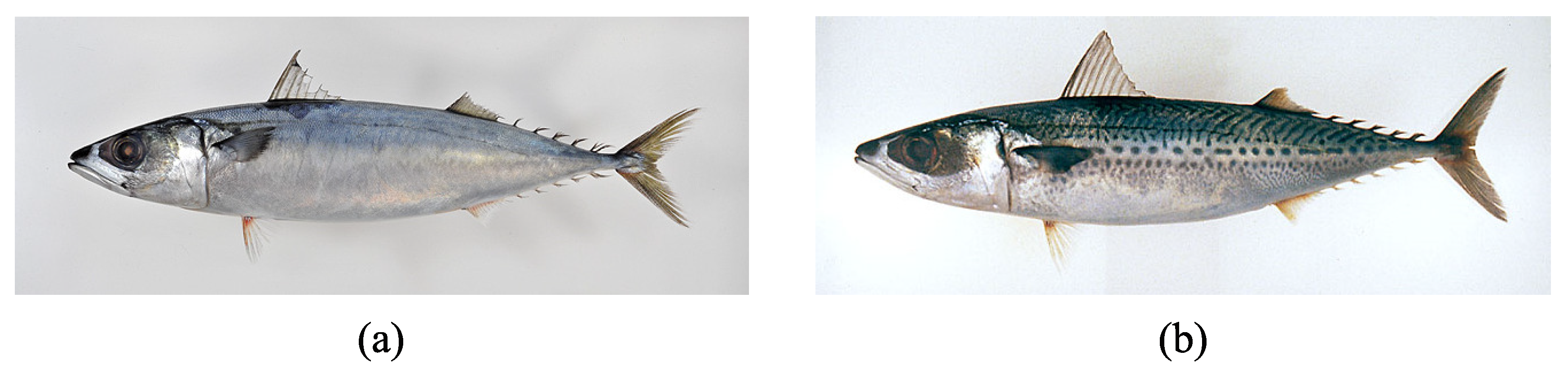
Mackerel is a major aquatic resource worldwide. In Japan, Scomber japonicus (chub mackerel) and Scomber australasicus (blue mackerel) shown in Figure 1 are the two most common species, primarily caught together along the coasts [1]. The former has a far higher market price than the latter, necessitating discrimination before shipment.
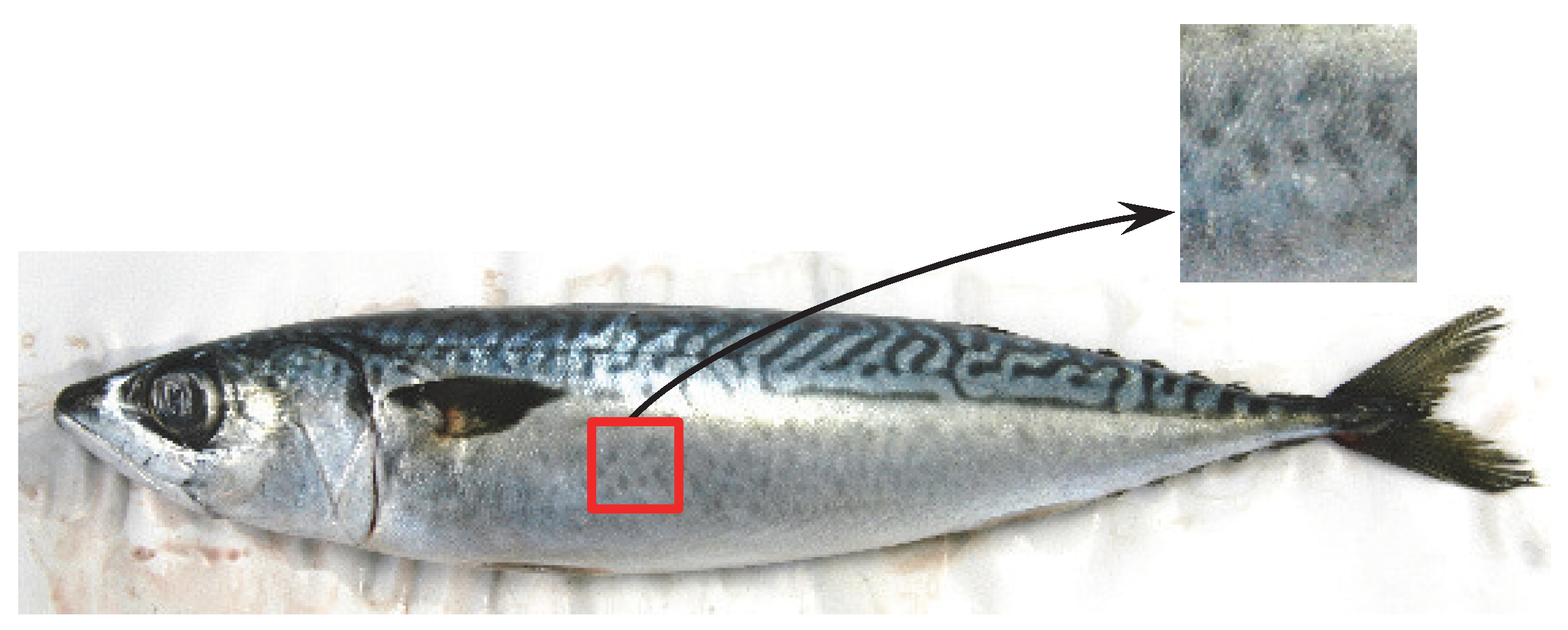
A typical difference between these two species is the textural feature on the ventral portion of their sides. In S. japonicus, this area is silver-white, whereas S. australasicus has spot patterns. In addition, the front view of S. japonicus is elliptical, while that of S. australasicus is circular. Generally, the fishing industry separates the mackerel based on these visible characteristics. However, some individuals have characteristics of both species and are difficult to discriminate even for experts (e.g., Figure 2).
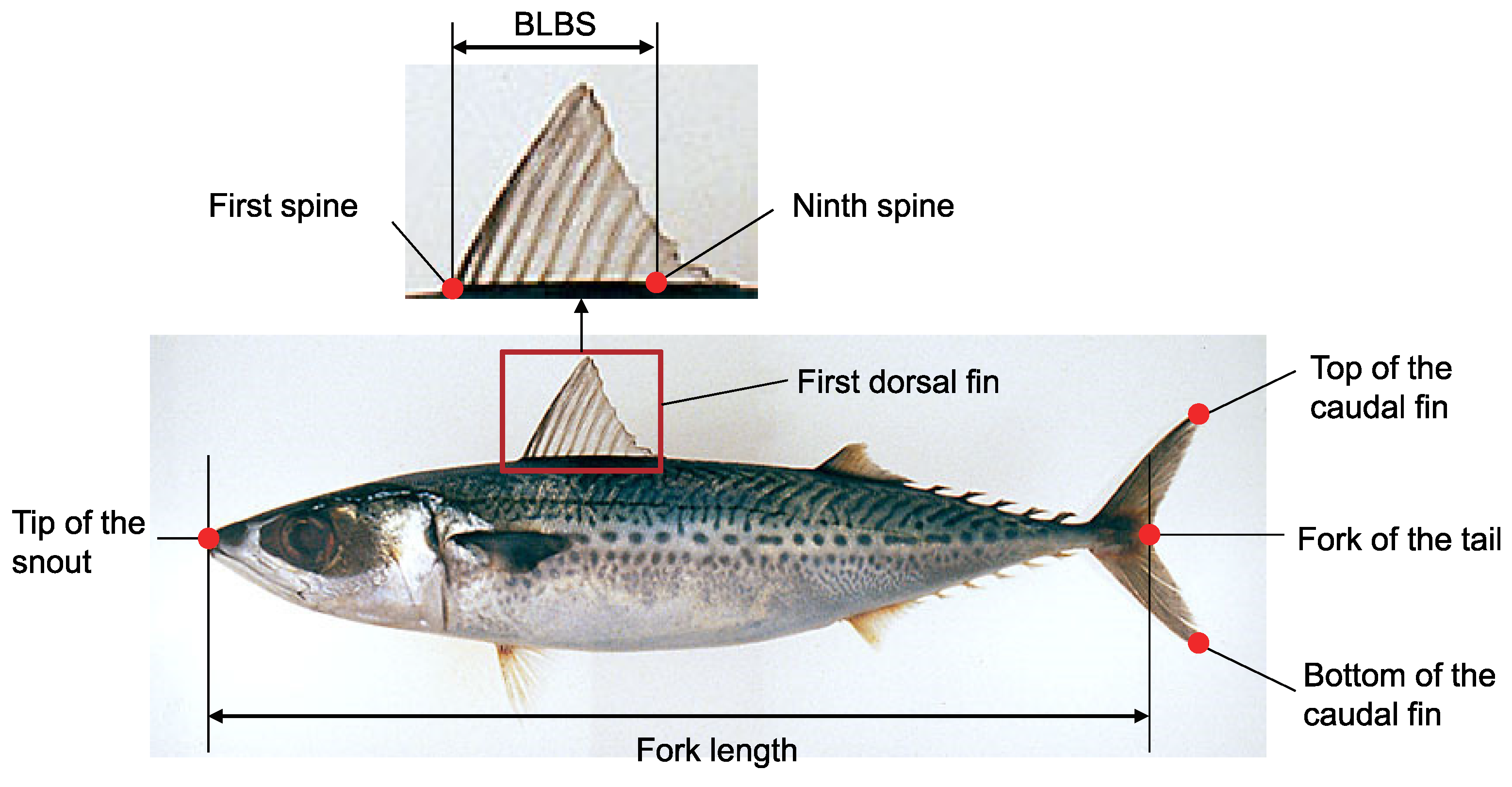
The two species also tend to differ in the characteristics of the first dorsal fin, with S. japonicus generally possessing 9 or 10 spines, while S. australasicus has 10 to 13 spines [2]. However, this method of discrimination is not always reliable because spine number exhibits some individual variation. Of the available options, the most accurate identification method is to first determine the base length between the first dorsal fin’s first and ninth spines (or the base length between spines (BLBS)), and then calculating the ratio of BLBS to the fork length (see Figure 3). If the ratio is greater than 0.12, the fish is S. japonicus otherwise, it is S. australasicus. According to the report by the National Research Institute of Fisheries Science in Japan [3], this method has an accuracy of about 99%. In our previous study presented at a workshop [4], we verified the effectiveness of this method by manually detecting fin region.
However, these measurements are performed manually on individual fish, which is a laborious process that can also decrease freshness. Therefore, it is not suitable for quickly separating a large mackerel catch, and the fish industry would benefit from an automatic identification method.
Related Work
Some studies have examined techniques for automatic discrimination between fish. The existing methods are roughly classified into two types.
The first is more relevant for marine biology, aiming to detect and classify fish underwater. For example, a deformable template [5] can be applied that matches fish based on the shape context [6] and distance transformation [7]. A system is also available for detecting, tracking, and classifying fish in behavioral studies [8]. Fish was first detected through a combination of a Gaussian mixture model and a moving average algorithm. Next, fish were classified using texture features derived from Gabor filters and gray level co-occurrence matrix (GLCM) [9], as well as shape features calculated with the curvature scale space transformation [10]. Contour detection has also been applied to fish [11], specifically using the Canny edge detector [12] and blob detection with the Laplacian of Gaussian filter, before final species identification with Zernike moments [13]. A combination of detection with Gaussian mixture models and tracking by the Kalman filter has been used as well [14], with subsequent species identification performed using a pyramid histogram of visual words (PHOV) [15]. Hasija et al. [16] classified fish species based on image-set matching with subspaces; accuracy was improved through discriminant analysis plus graphical representation.
The second type of research has greater industrial application because it is aimed at discriminating individual caught fish. Fouad et al. developed a machine-learning method for discriminating Nile tilapia from other Nile-River fishes [17]. Both scale invariant feature transformation (SIFT) [18] and speeded up robust features (SURF) [19] were separately applied to extract distinct features from a whole image of the fish. Next, artificial neural networks (ANN), K-nearest neighbor (K-NN), and support vector machines (SVM) [20] were employed to separate the Nile tilapia from other species. The results indicated that the combination of SURF and SVM achieved extremely high accuracy. Rodrigues et al. proposed five schemes for fish classification [21]. Distinguishing features were identified using principal component analysis (PCA), SIFT , and vector of locally aggregated descriptors [22]. Identified features were then clustered with artificial immune networks (aiNet) [23], adaptive radius immune algorithms (ARIA) [24], and k-means algorithms.The results indicated that PCA was the most effective for feature identification, while aiNet or ARIA were best for clustering. A classification method for three types of tuna—bigeye, yellowfin, and skipjack—was developed using decision trees with shape and texture features [25]. The circular rate of the head was selected as a shape feature. Next, GLCM was used to extract texture features, including contrast, correlation, energy, and other relevant factors. Based on a decision tree constructed with the extracted features, test images were classified into one of the three tuna. The study employed texture features because skipjacks have a distinctive characteristic of multiple linear patterns on the abdomen.
All of the existing techniques used texture features or the fish’s rough shape for discrimination. However, since the appearances of S. japonicus and S. australasicus are very similar, it is difficult to discriminate them by these features only. In this study, we propose an accurate discrimination method for mackerel using both textural and geometric features from the first dorsal fin. The proposed approach is in the second category described above.
2. Materials and Methods
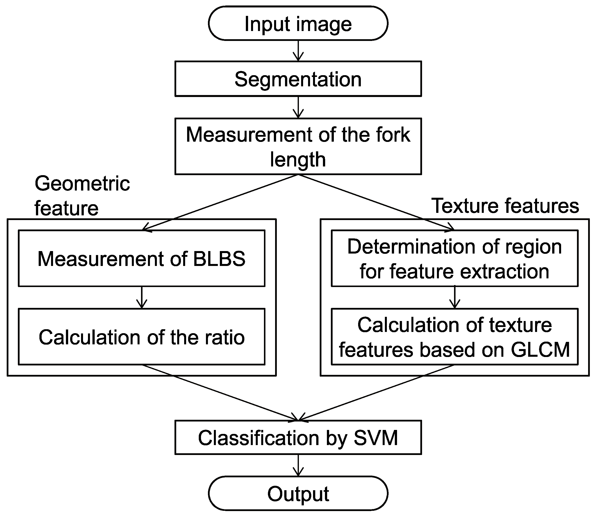
The flow of the proposed method is shown in Figure 4. First, segmentation is performed on a given input image and fish location is determined, followed by fork-length measurement. Next, geometric and texture features are extracted from the image. Specifically, the relevant geometric feature is the ratio of BLBS to fork length, while the texture feature is calculated based on the GLCM in the ventral half of the fish’s side. The two features are then combined and used for classification with the SVM. Below, we describe the details of each step.
2.1. Input
Input images are RGB color photographs of a mackerel laid horizontally with its head on the viewer’s left. Examples are shown in Figure 1.
2.2. Segmentation
Edge detection and mathematical morphology techniques [26] (e.g., dilation and erosion) are used for segmentation. First, the input image is converted to gray scale for edge detection with the Sobel filter [27]. Figure 5a shows the results of edge detection on the image in Figure 1b, revealing the fish’s contours clearly.
Next, dilation is applied to two vertically adjacent and then two horizontally adjacent pixels. The resultant hole is filled with the edge pixel value, and the pixel touching the image boundary is erased. Figure 5b shows a representative result of dilation, wherein the fish area was roughly extracted.
The dilation-derived fish area is larger than the actual area and some noise pixels exist. Therefore, erosion is applied for three times for each pixel and its four-neighbor pixels, thus completing segmentation. As seen in the final segmentation image (Figure 5c), erosion eliminated noise, resulting in an area that was approximately the same as the fish’s actual size.
Finally, fish location is estimated from this finalized image. The smallest rectangle surrounding each connected component is identified and its area is calculated. Fish location is set as the connected component with the largest surrounding rectangle (Figure 5d).
2.3. Fork-Length Measurement
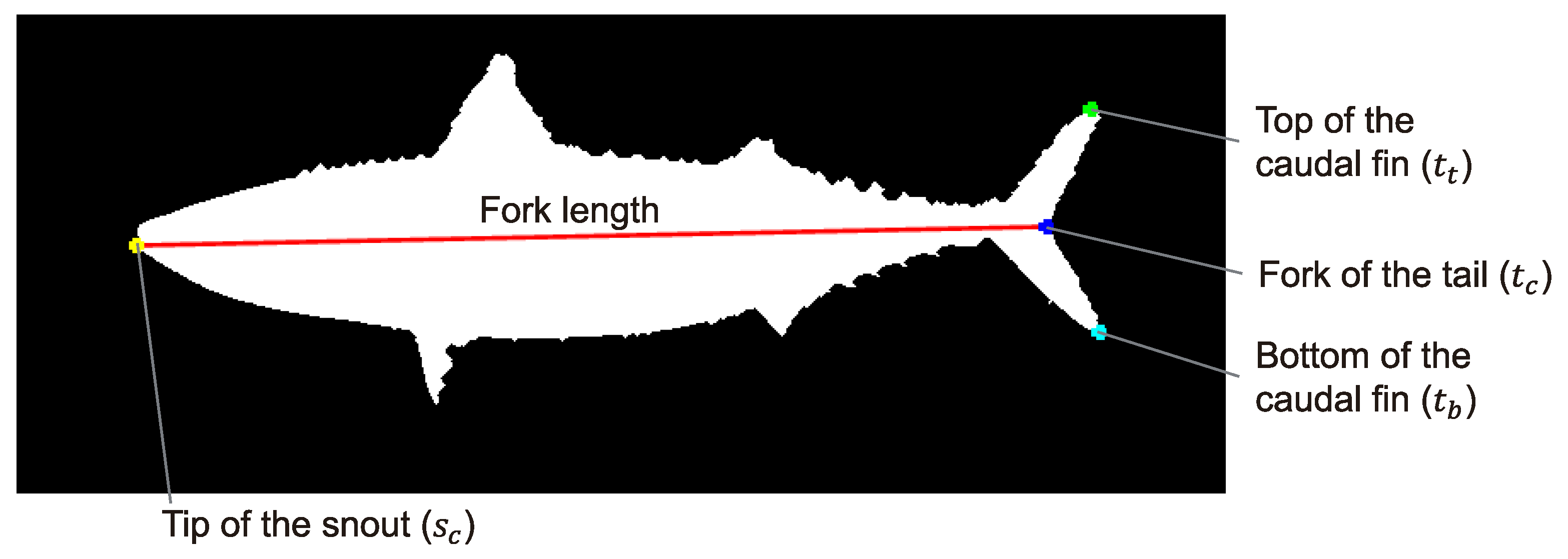
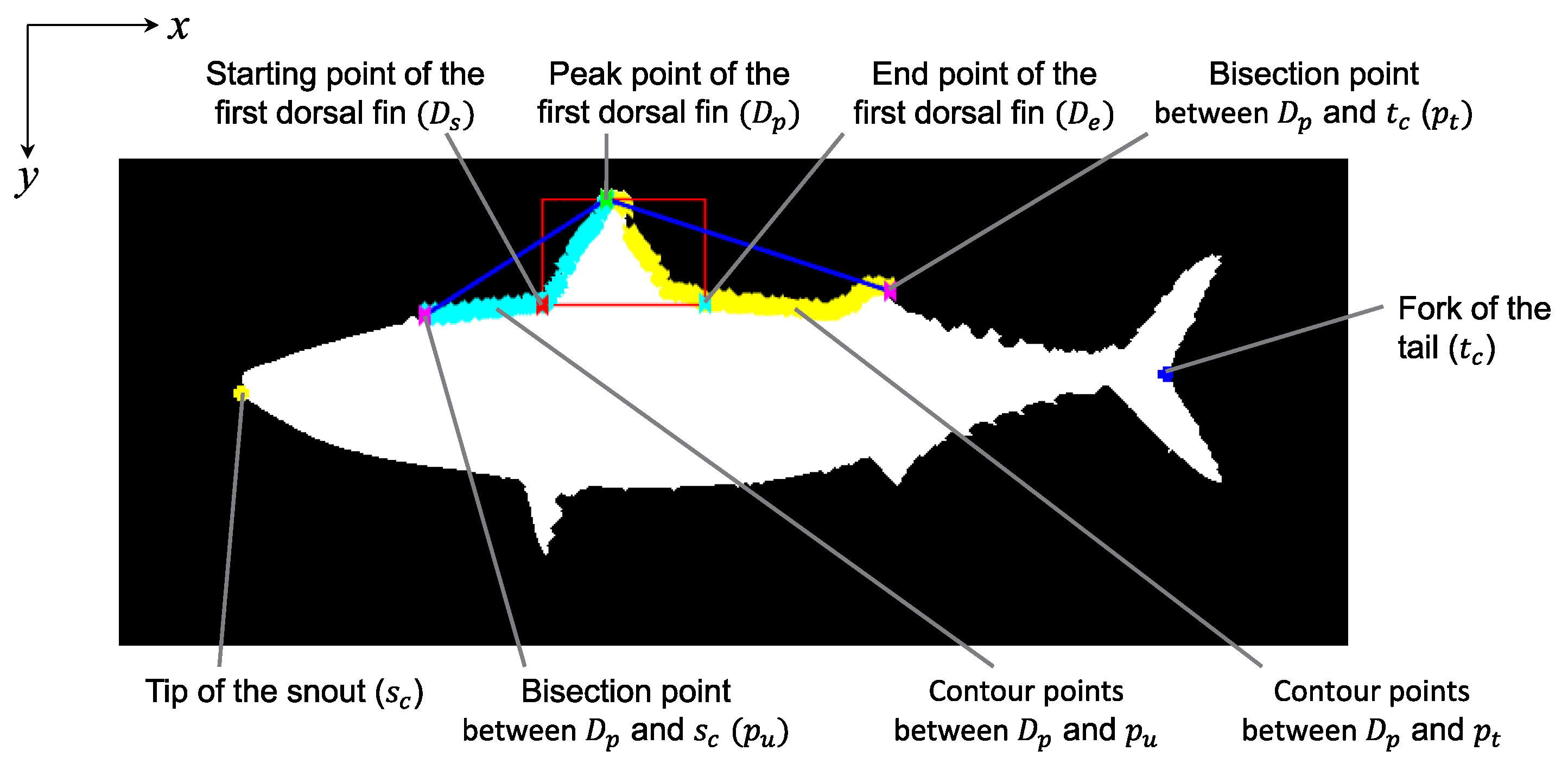
Fork length is measured from the tip of the snout () to the fork of the tail () (Figure 6). Thus, these points are first identified in the image as follows.
The distance from the upper right corner of the input image to each contour point is calculated. The minimum-distance contour point is considered the top of the caudal fin (). Similarly, the bottom of the caudal fin () is determined based on the distance from the lower right corner of the input image. The fork of the tail () is determined as the leftmost contour point moving from to in a clockwise direction. The tip of the snout () is determined as the maximum-distance point from . Finally, the fork length is calculated as the distance between and .
2.4. Measurement of Base Length between Spines
This measurement involves rough detection of the first dorsal fin, followed by the positions of the spines. The base length between the first and ninth spines (BLBS) is then calculated.
2.4.1. Rough Detection of First Dorsal Fin
First, the region of the first dorsal fin is roughly detected from the input image, by identifying the peak (), starting (), and end () points of the first dorsal fin (Figure 7). The peak point () is the contour point with the minimum y-coordinate. Next, is on the contour and has the same x-coordinate as the point bisecting the line segment connecting and . The starting point of the first dorsal fin () is the farthest point on the contour from the straight line connecting and . Similarly, is on the contour and has the same x-coordinate as the point bisecting the line segment connecting and . Lastly, the end of the first dorsal fin () is the farthest point on the contour between and from the straight line through both points.
The rough region of the first dorsal fin is then detected as the rectangular region defined by , , and (red rectangle in Figure 7). The bottom of this region is the larger y-coordinate when comparing and . This region is called fin-region hereafter.
2.4.2. Detection of Spine Positions
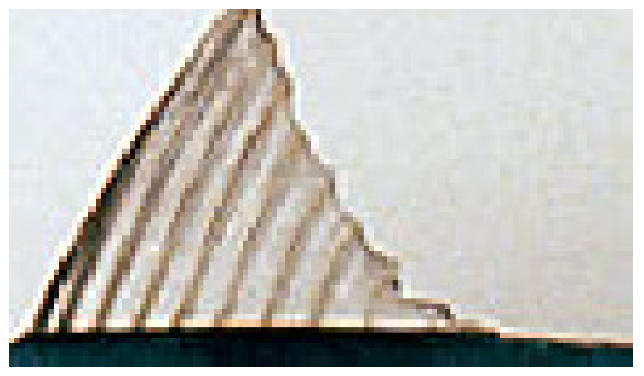
Next, spines are detected considering the detected fin-region. Let the height and the width of the fin-region be h and , respectively. Since is often not exactly the end point of the dorsal fin, we set the lateral length of the region where spines are detected longer than that of the fin-region while the leftmost point is fixed to . If is smaller than 1.05 (This corresponds to a case where a part of the fin is missing), the region’s width w is calculated as . Otherwise, it was calculated as . An example of the region where spines were detected is shown in Figure 8.
Then we apply Gaussian smoothing to binarize the image. Binarization is performed following a method based on Niblack’s local thresholding [28]. This procedure determines a threshold for each pixel based on a small region surrounding said pixel. Here, the threshold of pixel is defined as
where and are the mean and standard deviation of the small region surrounding pixel , while k and are parameters defined as and . In the original Niblack’s method, . The small region is set as pixels centered at . If the pixel value of the smoothed image is larger than the threshold , it is considered part of the spine region. Connected components with less than five pixels are deleted as noise, and holes generated via the binarization process are filled. The binarized image of Figure 8 is displayed in Figure 9.
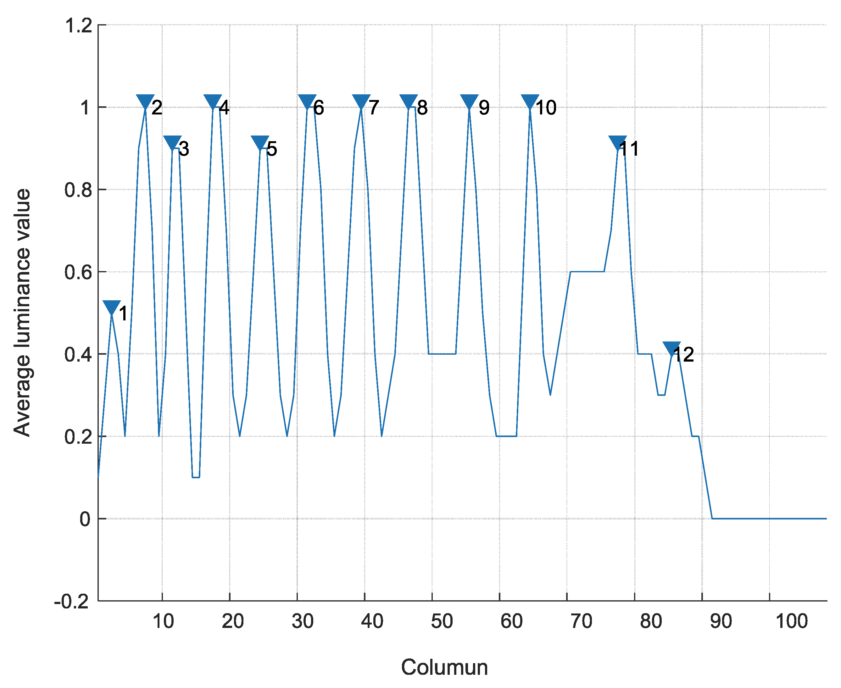
Next, the number of white pixels in each row of the binarized image is counted. If the number is greater than four-fifths of the input width, the row is excluded from histogram construction (for an example, see the blue rectangle in Figure 9). The remaining bottom region is then extracted so that it has a height that was 7% of the image height (red rectangle in Figure 9). To detect each spine, a luminance histogram (Figure 10) is generated as the average of the pixel values per column in the red rectangle. The histogram is then smoothed using the moving average method (window size = 2).
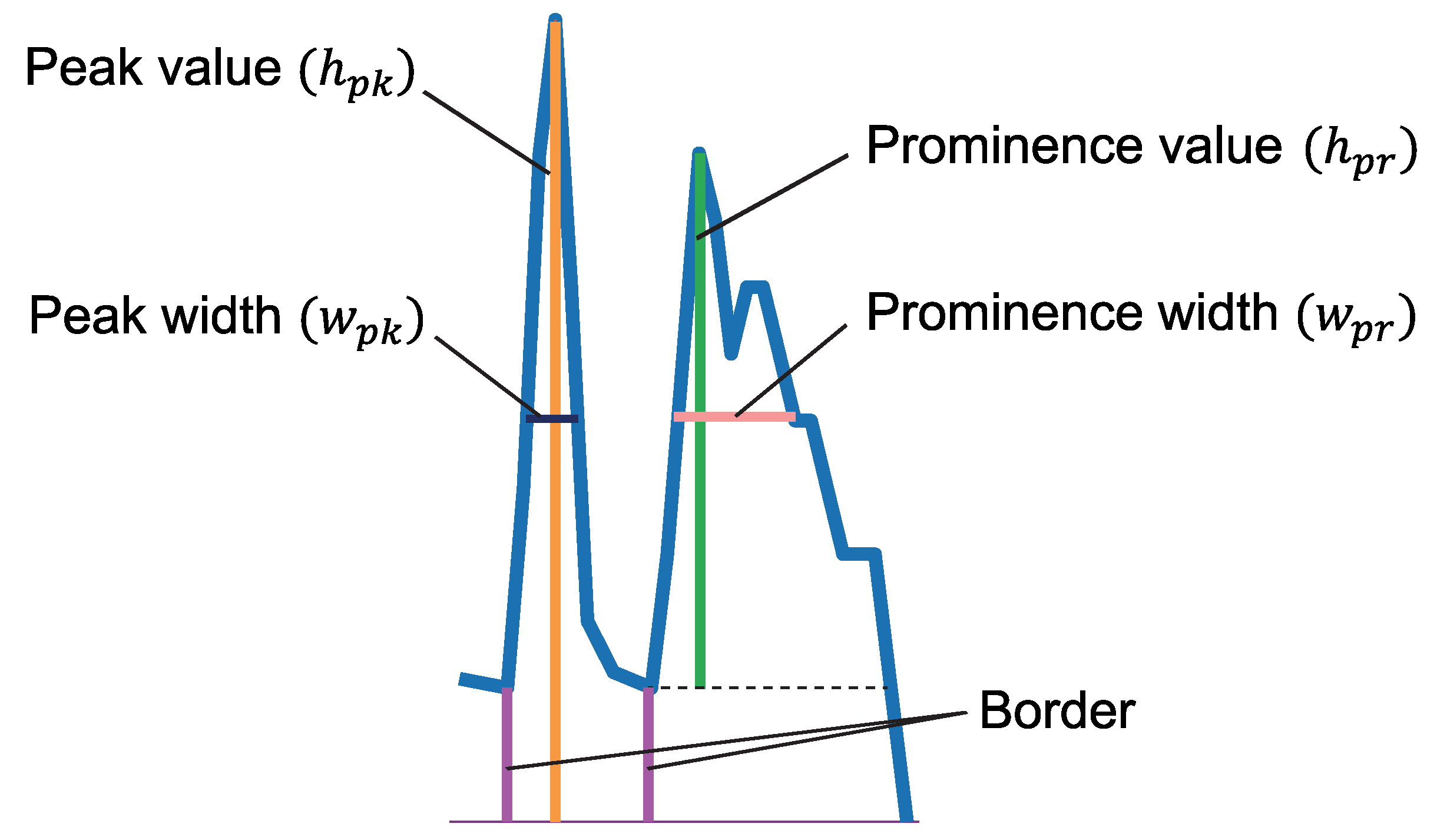
The histogram’s peaks represent the spines. First, peak () and prominence () values per histogram peak are calculated (see Figure 11). The prominence value is defined as the height from the higher level of adjacent valley or endpoint to the peak. Next, peak () and prominence () widths are determined. The peak width is defined by the intersections of the horizontal line at the peak’s half height and the signal or border, where the border represents the horizontal position of the valley. The prominence width is defined by the intersections of the horizontal line at the half prominence and the signal. Peaks meeting the following thresholds: , , and are discarded in advance as noise. In addition, peaks that satisfy the following three conditions are also discarded as being too small.
where , , and are the median values of all prominence values, prominence widths, and peak widths, respectively. The values of parameters , and are determined in advance.
In the binarization process, there are cases in which two spines are connected and extracted as one peak. If the following condition is satisfied, the peak is regarded to include two spines.
where is a parameter. In addition, when the second peak satisfies , if the distance between the peak and its previous peak is larger than 1.48 times the distance between the peak and its following peak, the peak is regarded to include two spines.
On the contrary, peaks that do not correspond to spines are deleted. We determine whether this is the case through measuring the interval between spines, which tends to grow gradually larger. Thus, each peak after the second one is discarded if the ratio of peak-to-following-peak distance and peak-to-previous-peak distance is less than 0.64.
The peak corresponding to the ninth spine can be difficult to discern from the luminance histogram because that spine tends to be very short or buried in the body. Therefore, when we only detect eight spines, we estimate the ninth spine’s position by adding the interval between the seventh and eighth spines to the position of the eighth spine.
Next, the position of the ninth spine is slightly adjusted. If the ratio of the eighth-to-ninth-peak interval to the seventh-to-eighth-peak interval is greater than 1.1, then the position is moved left by one-fourth the distance between the eighth and ninth peaks. When eight peaks are detected, the position of the eighth spine is moved left by a quarter of the distance between the seventh and eighth peaks, if the ratio between the seventh-to-eight interval and the sixth-to-seventh interval is greater than 1.5.
Finally, BLBS is measured based on the positions of the first and ninth spines, allowing calculation of the BLBS to fork length ratio as the discriminating geometric feature.
2.5. Texture Feature Extraction
First, we determine the region for extracting texture features. Because S. australasicus spot patterns are on the ventral portion of the side, we block off this region by first delineating its upper left point as where the fork length is internally divided into 3:5 and then shifted by ; H is the height of the fish. The width and height of the region are respectively and , where FL is the fork length. These values were determined by observing standard mackerels. An example of the finalized region is shown in Figure 12. This area includes the spot pattern necessary to discriminate between S. japonicus and S. australasicus.
Texture features are extracted from the designated area based on the GLCM [9]. In this matrix, element represents the probability , given as a parameter. Here, is the probability that a given pixel intensity is i and another pixel’s intensity is j, where the distance between these pixels is d, and the angle between the line connecting the two pixels and a horizontal line is (Figure 13). The value of can be , , , or . This study uses five texture features: contrast, correlation, energy, homogeneity, and entropy. Contrast is a difference in intensity between neighboring pixels (the larger the contrast, the greater the intensity difference). Correlation is the linear dependence of intensities between neighboring pixels. A higher value indicates that there are pixels with similar intensity values in a specific direction. Energy is the uniformity between neighboring pixels. A high-energy value shows that more pixels and patterns of specific intensity values are in the image. Homogeneity is the similarity between neighboring pixels; thus, the image has more pixels with similar intensity values if homogeneity values are high. Entropy is the randomness between neighboring pixels; greater entropy indicates that more pixels with different intensity values are present in the image. Table 1 shows the parameters for calculating each feature.
3. Results and Discussion
We performed experiments on 19 images of S. japonicus and 18 images of S. australasicus. Thirty-three of these images were from the fish dataset FishPix [29] of the Kanagawa Prefectural Museum of Natural History. Figure 1 depicts an example image used for the experiment.
The first experiment isolated features effective for discrimination from a pool of all GLCM features. Because the number of images in the dataset was insufficient, we used double cross-validation to determine SVM parameters and to allow model learning. The dataset was subdivided into and . included 19 images (10 S. japonicus images and 9 S. australasicus images), while includes 18 images (9 S. japonicus images and 9 S. australasicus images). First, we performed a leave-one-out experiment to determine SVM parameters using dataset . Next, we used those SVM parameters to perform another leave-one-out experiment that classified each image in . The same process was repeated with the datasets switched. We calculated the accuracy via integrating these two results (Table 2). Linear and radial basis function (RBF) kernels were used separately for the SVM.
When combining contrast and homogeneity as the texture feature, 84% accuracy was obtained, the highest value we observed (higher than using all textures). Furthermore, RBF was consistently better than linear kernel. Therefore, we combined contrast and homogeneity as the texture feature, and selected the RBF kernel for SVM.
Next, the accuracy of the proposed method was verified through a comparison with a closely related, previously published technique [25]. For fair comparison, texture features described in Section 2.5 were also used for the existing method. We performed a leave-one-out analysis and trained the classifier with 36 out of 37 images. The remaining image was then subjected to the classifier. The parameters used in the experiments were determined as shown in Table 3.
The results are shown in Table 4. The proposed method achieved a far higher accuracy than the Khotimah et al. method, verifying the former’s effectiveness.
Figure 14 shows an example that was not correctly classified by the proposed method. This S. australasicusw̃as inaccurately identified as S. japonicus. The misclassification was likely due to poor BLBS measurements. In this specimen, the peak of the second spine could not be detected due to the spines’ close proximity. In addition, the spot pattern on the body was very faint, resulting in a texture feature that was similar to S. japonicus. Thus, to improve accuracy, future studies should aim to find a texture feature that can distinguish between the two mackerel even when specimens have faint spot patterns.
4. Conclusions
In this study, we proposed a novel method for discriminating S. japonicus and S. australasicus, using a combination of geometric and texture features extracted from standardized images. We used the BLBS to fork length ratio as the distinguishing geometric feature, as well as GLCM-calculated constant and homogeneity values as the texture feature. Mackerels were then classified based on these features, using SVM with the RBF kernel.
Experimental results verified the effectiveness of the proposed method. Due to issues during image acquirement, we observed several cases where the texture feature was unclear or the length measurement failed. However, even in such cases, the proposed method was capable of separating fish robustly because both features were always taken into account.
This time we showed experimental results with a small dataset because as far as we know there are few public datasets of S. japonicus and S. australasicus labelled by experts. Conducting verification experiments using a larger datasets and showing the statistical properties of the proposed method is a future work.
In addition, we determined some parameter values manually because we did not have enough data for statistical determination. Therefore, the values were not optimal ones. An important future task would be to obtain optimal parameter values using techniques such as machine learning with a far greater variety of images.
Author Contributions
Funding acquisition, S.O.; Methodology, A.K.; Project administration, S.O.; Software, A.K.; Supervision, T.M. and Y.S.; Validation, T.M. and Y.S.; Writing—original draft, A.K.; Writing—review & editing, S.O.
Funding
This work was partially supported by JSPS KAKENHI Grant Number JP16K00259.
Acknowledgments
The authors would like to thank the Kanagawa Prefectural Museum of Natural History for providing the fish images. The images used for the experiments are recorded under the following material numbers. S. japonicus: KPM-NR 868, KPM-NR 869, KPM-NR 887, KPM-NR 2750, KPM-NR 48264, KPM-NR 49744, KPM-NR 53219, KPM-NR 57070, KPM-NR 57234, KPM-NR 57235, KPM-NR 57236, KPM-NR 59801, KPM-NR 93972, KPM-NR 106607, KPM-NR 106851, KPM-NR 106909, KPM-NR 106910, KPM-NR 108549, KPM-NR 108563. S. australasicus: KPM-NR 1056, KPM-NR 20548, KPM-NR 49745, KPM-NR 53217, KPM-NR 53218, KPM-NR 55609, KPM-NR 55610, KPM-NR 55611, KPM-NR 58903, KPM-NR 59849, KPM-NR 90341, KPM-NR 106608, KPM-NR 108560, KPM-NR 108807. Images used as the figures are archived as follows. Figure 1a: KPM-NR 106607. Figure 1b, Figure 3, Figure 5, Figure 6, Figure 7, Figure 8 and Figure 9 and Figure 12: KPM-NR 55609. Figure 14: KPM-NR 108807. (Photo: Hiroshi Senou, Kanagawa Prefectural Museum of Natural History)
Conflicts of Interest
The authors declare no conflict of interest.
References
- Sassa, C.; Tsukamoto, Y. Distribution and growth of Scomber japonicus and S. australasicus larvae in the southern East China Sea in response to oceanographic conditions. Mar. Ecol. Prog. Ser. 2010, 419, 185–199. [Google Scholar] [CrossRef]
- Baker, E.A.; Collette, B.B. Mackerel from the northern Indian Ocean and the Red Sea are Scomber australasicus, not Scomber japonicus. Ichthyol. Res. 1998, 45, 29–33. [Google Scholar] [CrossRef]
- National Research Institute of Fisheries Science. Manual for Discrimination of Scomber Japonicus and Scomber Australasicus (Masaba Gomasaba Hanbetsu Manyuaru); National Research Institute of Fisheries Science: Yokohama, Japan, 1999. (In Japanese)
- Kitasato, A.; Miyazaki, T.; Sugaya, Y.; Omachi, S. Discrimination of Scomber japonicus and Scomber australasicus by dorsal fin length and fork length. In Proceedings of the 22nd Korea-Japan joint Workshop on Frontiers of Computer Vision, Takayama, Japan, 17–19 February 2016; pp. 338–341. [Google Scholar]
- Rova, A.; Mori, G.; Dill, L.M. One fish, two fish, butterfish, trumpeter: Recognizing fish in underwater video. In Proceedings of the IAPR Conference on Machine Vision Applications, Nagoya, Japan, 8–12 May 2017; pp. 404–407. [Google Scholar]
- Belongie, S.; Malik, J.; Puzicha, J. Shape matching and object recognition using shape contexts. IEEE Trans. Pattern Anal. Mach. Intell. 2002, 24, 509–522. [Google Scholar] [CrossRef] [Green Version]
- Felzenszwalb, P.F.; Huttenlocher, D.P. Pictorial structures for object recognition. Int. J. Comput. Vis. 2005, 61, 55–79. [Google Scholar] [CrossRef]
- Spampinato, C.; Giordano, D.; Di Salvo, R.; Chen-Burger, Y.; Fisher, R.B.; Nadarajan, G. Automatic fish classification for underwater species behavior understanding. In Proceedings of the First ACM International Workshop on Analysis and Retrieval of Tracked Events and Motion in Imagery Streams, Firenze, Italy, 25–29 October 2010; pp. 45–50. [Google Scholar]
- Haralick, R.M.; Shanmugan, K.; Dinstein, I. Textural features for image classification. IEEE Trans. Syst. Man Cybern. 1973, SMC-3, 610–621. [Google Scholar] [CrossRef]
- Mokhtarian, F.; Abbasi, S. Shape similarity retrieval under affine transforms. Pattern Recognit. 2002, 35, 31–41. [Google Scholar] [CrossRef]
- Fabic, J.N.; Turla, I.E.; Capacillo, J.A.; David, L.T.; Naval, P.C. Fish population estimation and species classification from underwater video sequences using blob counting and shape analysis. In Proceedings of the 2013 IEEE International Underwater Technology Symposium, Tokyo, Japan, 5–8 March 2013. [Google Scholar]
- Canny, J. A computational approach to edge detection. IEEE Trans. Pattern Anal. Mach. Intell. 1986, PAMI-8, 679–698. [Google Scholar] [CrossRef]
- Khotanzad, A.; Hong, Y.H. Invariant image recognition by Zernike moments. IEEE Trans. Pattern Anal. Mach. Intell. 1990, 12, 489–497. [Google Scholar] [CrossRef]
- Hossain, E.; Alam, S.M.S.; Ali, A.A.; Amin, M.A. Fish activity tracking and species identification in underwater video. In Proceedings of the 5th International Conference on Informatics, Electronics and Vision, Dhaka, Bangladesh, 13–14 May 2016. [Google Scholar]
- Bosch, A.; Zisserman, A.; Muñoz, X. Image classification using random forests and ferns. In Proceedings of the IEEE 11th International Conference on Computer Vision, Rio de Janeiro, Brazil, 14–21 October 2007. [Google Scholar]
- Hasija, S.; Buragohain, M.J.; Indu, S. Fish species classification using graph embedding discriminant analysis. In Proceedings of the International Conference on Machine Vision and Information Technology, Singapore, 7–19 February 2017; pp. 81–86. [Google Scholar]
- Fouad, M.M.M.; Zawbaa, H.M.; El-Bendary, N.; Hassanien, A.E. Automatic Nile Tilapia fish classification approach using machine learning techniques. In Proceedings of the 13th International Conference on Hybrid Intelligent Systems, Gammarth, Tunisia, 4–6 December 2013; pp. 173–178. [Google Scholar]
- Lowe, D.G. Distinctive image features from scale-invariant keypoints. Int. J. Comput. Vis. 2004, 60, 91–110. [Google Scholar] [CrossRef]
- Bay, H.; Ess, A.; Tuytelaars, T.; Van Gool, L. Speeded-up robust features. Comput. Vis. Image Underst. 2008, 110, 346–359. [Google Scholar] [CrossRef]
- Vapnik, V.N. Statistical Learning Theory; John Wiley & Sons: Hoboken, NJ, USA, 1998. [Google Scholar]
- Rodrigues, M.T.A.; Freitas, M.H.G.; Pádua, F.L.C.; Gomes, R.M.; Carrano, E.G. Evaluating cluster detection algorithms and feature extraction techniques in automatic classification of fish species. Pattern Anal. Appl. 2015, 18, 783–797. [Google Scholar] [CrossRef]
- Jégou, H.; Douze, M.; Schmid, C.; Pérez, P. Aggregating local descriptors into a compact image representation. In Proceedings of the 2010 IEEE Conference on Computer Vision and Pattern Recognition, San Francisco, CA, USA, 13–18 June 2010; pp. 3304–3311. [Google Scholar]
- De Castro, L.N.; Von Zuben, F.J. aiNet: An Artificial Immune Network for Data Analysis. In Data Mining: A Heuristic Approach; Idea Group Inc.: London, UK, 2002; pp. 231–260. [Google Scholar]
- Bezerra, G.B.; Barra, T.V.; de Castro, L.N.; Von Zuben, F.J. Adaptive radius immune algorithm for data clustering. In Lecture Notes in Computer Science; Springer: Heidelberg/Berlin, Germany, 2005; pp. 290–303. [Google Scholar]
- Khotimah, W.N.; Arifin, A.Z.; Yuniarti, A.; Wijaya, A.Y.; Navastara, D.A.; Kalbuadi, M.A. Tuna fish classification using decision tree algorithm and image processing method. In Proceedings of the International Conference on Computer, Control, Informatics and Its Applications, Bandung, Indonesia, 5–7 October 2015; pp. 126–131. [Google Scholar]
- Najman, L.; Talbot, H. Mathematical Morphology; Wiley-ISTE: Washington, DC, USA, 2013. [Google Scholar]
- Szeliski, R. Computer Vision; Springer: Heidelberg/Berlin, Germany, 2010. [Google Scholar]
- Niblack, W. An Introduction to Digital Image Processing; Prentice Hall: Upper Saddle River, NJ, USA, 1986. [Google Scholar]
- FishPix. Available online: http://fishpix.kahaku.go.jp/fishimage-e/index.html (accessed on 27 June 2018).
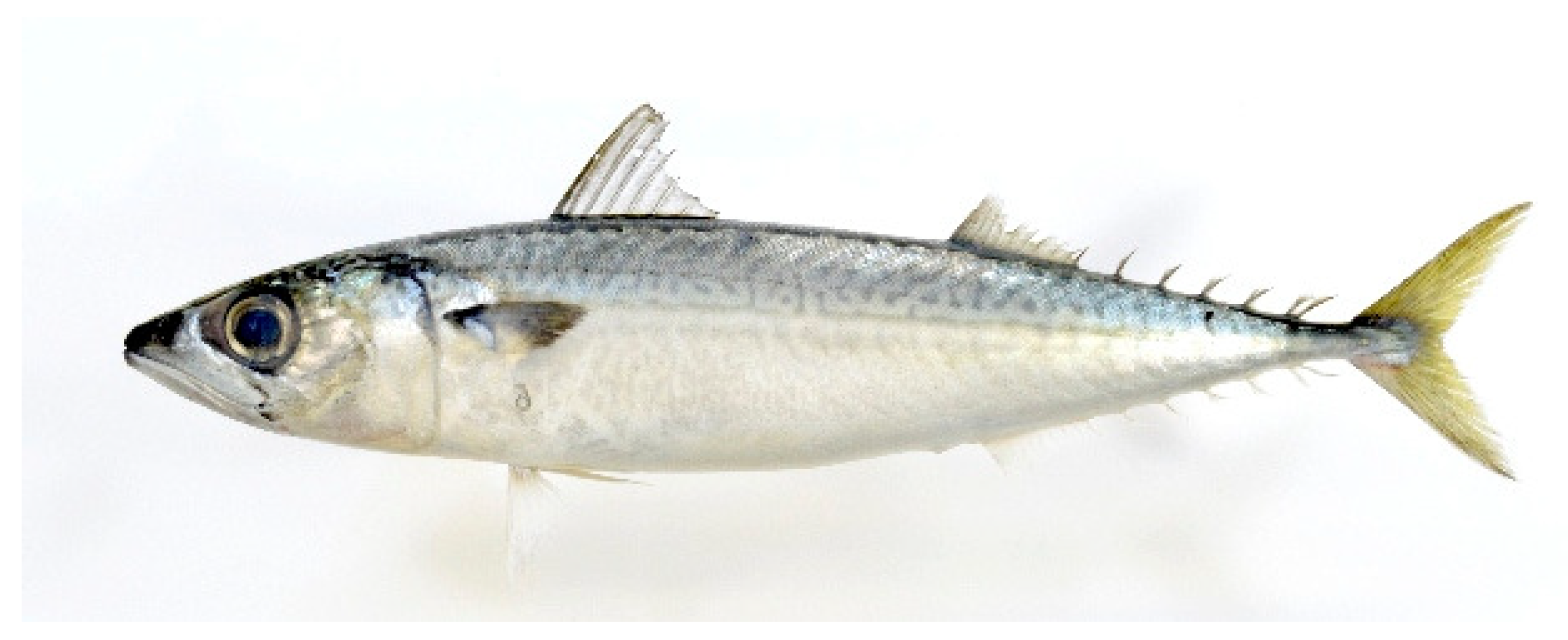
Figure 1.
Two major mackerel species caught on Japanese coasts. (a) Scomber japonicus (chub mackerel); (b) Scomber australasicus (blue mackerel).
Figure 1.
Two major mackerel species caught on Japanese coasts. (a) Scomber japonicus (chub mackerel); (b) Scomber australasicus (blue mackerel).

Figure 2.
A mackerel that is difficult to classify. The specimen looks like S. japonicus, but has light spot patterns which is characteristic of S. australasicus.
Figure 2.
A mackerel that is difficult to classify. The specimen looks like S. japonicus, but has light spot patterns which is characteristic of S. australasicus.

Figure 3.
The base length between the first and ninth spines of the first dorsal fin (BLBS) and the fork length.
Figure 3.
The base length between the first and ninth spines of the first dorsal fin (BLBS) and the fork length.

Figure 4.
Flow of the proposed discrimination method for S. japonicus and S. australasicus. GLCM: gray level co-ocurrence matrix; SVM: support vector machines.
Figure 4.
Flow of the proposed discrimination method for S. japonicus and S. australasicus. GLCM: gray level co-ocurrence matrix; SVM: support vector machines.

Figure 5.
Segmentation and estimation of fish location. (a) Edge detection; (b) dilation; (c) erosion; (d) location of fish represented by red rectangle.
Figure 5.
Segmentation and estimation of fish location. (a) Edge detection; (b) dilation; (c) erosion; (d) location of fish represented by red rectangle.
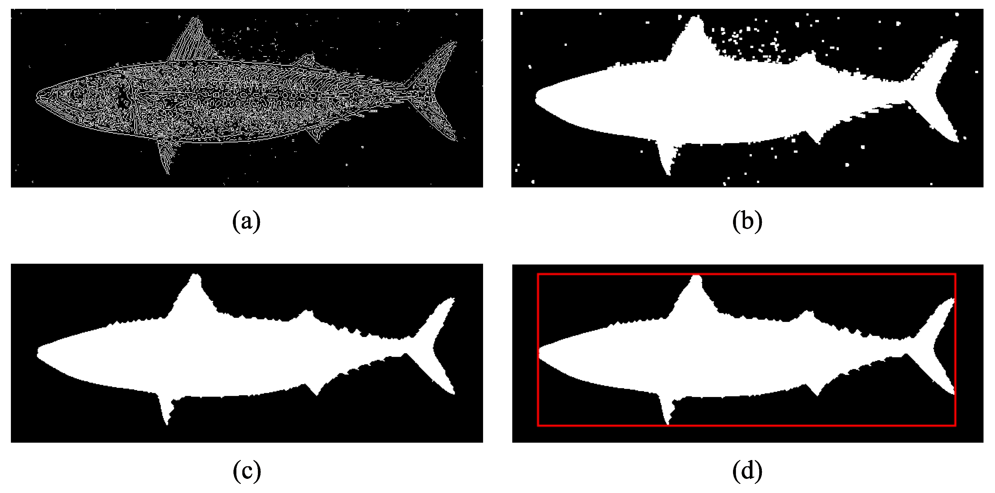
Figure 6.
Feature points used for measuring fork length.

Figure 7.
Feature points used to detect the first dorsal fin.

Figure 8.
The region where spines were detected.

Figure 9.
Binarized image of the first dorsal fin. White pixels indicate the spines. The region surrounded by the red rectangle was used for histogram construction.
Figure 9.
Binarized image of the first dorsal fin. White pixels indicate the spines. The region surrounded by the red rectangle was used for histogram construction.

Figure 10.
Histogram. The horizontal axis represents the image’s columns and the vertical axis shows the average luminance per column. Triangles indicate the ordinal number of each peak.
Figure 10.
Histogram. The horizontal axis represents the image’s columns and the vertical axis shows the average luminance per column. Triangles indicate the ordinal number of each peak.

Figure 11.
Peak value, peak width, prominence value, and prominence width of the histogram.

Figure 12.
Region where the texture features are extracted, blocked in a red rectangle.
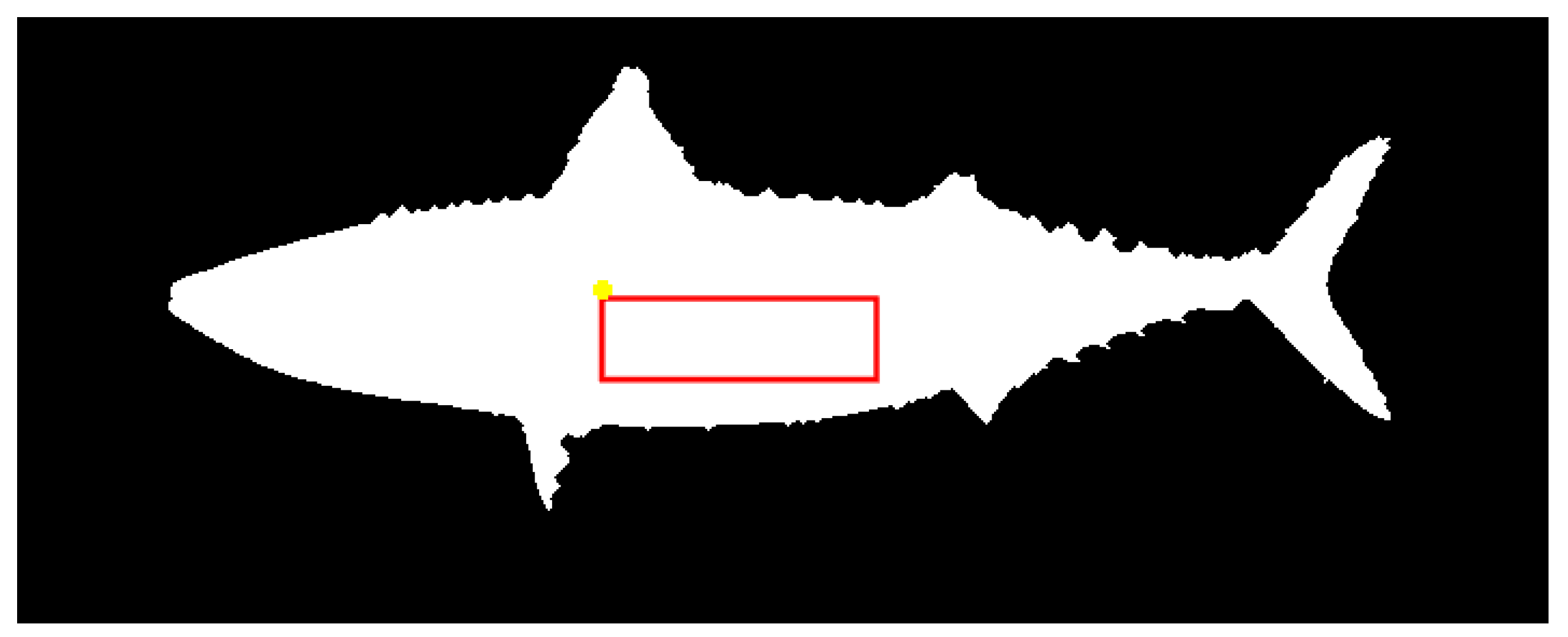
Figure 13.
Parameters for calculating the gray level co-occurrence matrix to determine texture features.
Figure 13.
Parameters for calculating the gray level co-occurrence matrix to determine texture features.
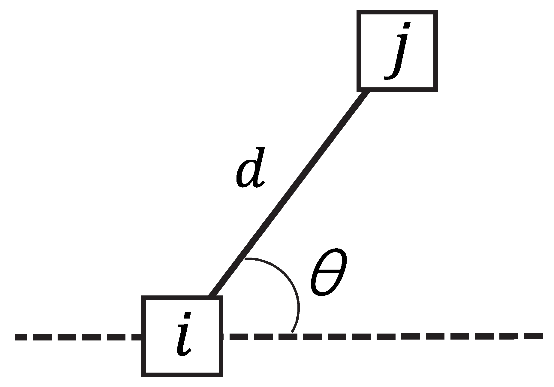
Figure 14.
An incorrectly classified mackerel.


Table 1.
Parameters for calculating features.
| Feature | d | |
|---|---|---|
| Contrast | 4 | |
| Correlation | 4 | |
| Energy | 1 | |
| Homogeneity | 4 | |
| Entropy | 4 |
Table 2.
Accuracy in classification using texture features and SVM. The columns RBF and Linear represent the accuracy when radial basis function kernel and linear kernel were used for the SVM, respectively.
Table 2.
Accuracy in classification using texture features and SVM. The columns RBF and Linear represent the accuracy when radial basis function kernel and linear kernel were used for the SVM, respectively.
| Texture feature | RBF | Linear |
|---|---|---|
| Contrast | 70% | 70% |
| Correlation | 65% | 62% |
| Energy | 70% | 62% |
| Homogeneity | 81% | 81% |
| Entropy | 70% | 68% |
| Contrast + Homogeneity | 84% | 84% |
| All textures | 76% | 76% |
Table 3.
Parameters used for the experiments.
| Parameter | Value |
|---|---|
| 0.51 | |
| 0.65 | |
| 0.85 | |
| 1.626 |
Table 4.
Comparison of classification accuracy between the proposed method and an existing, previously published method of fish discrimination. The row ratio only is the result of classifying the image based only on the BLBS to fork length ratio. The row texture only is the result of just using texture features.
| Method | Accuracy [%] |
|---|---|
| Proposed method | 97% |
| Ratio only | 89% |
| Texture only | 84% |
| Khotimah et al. [25] | 76% |
© 2018 by the authors. Licensee MDPI, Basel, Switzerland. This article is an open access article distributed under the terms and conditions of the Creative Commons Attribution (CC BY) license (http://creativecommons.org/licenses/by/4.0/).
Share and Cite
MDPI and ACS Style
Kitasato, A.; Miyazaki, T.; Sugaya, Y.; Omachi, S. Automatic Discrimination between Scomber japonicus and Scomber australasicus by Geometric and Texture Features. Fishes 2018, 3, 26. https://doi.org/10.3390/fishes3030026
AMA Style
Kitasato A, Miyazaki T, Sugaya Y, Omachi S. Automatic Discrimination between Scomber japonicus and Scomber australasicus by Geometric and Texture Features. Fishes. 2018; 3(3):26. https://doi.org/10.3390/fishes3030026
Chicago/Turabian StyleKitasato, Airi, Tomo Miyazaki, Yoshihiro Sugaya, and Shinichiro Omachi. 2018. "Automatic Discrimination between Scomber japonicus and Scomber australasicus by Geometric and Texture Features" Fishes 3, no. 3: 26. https://doi.org/10.3390/fishes3030026