A Statistical Regression Method for Characterization of Household Solid Waste: A Case Study of Awka Municipality in Nigeria


1
Shell Centre for Environmental Management and Control, University of Nigeria, Enugu Campus, Enugu 410001, Nigeria
2
Department of Mechanical Engineering, University of Nigeria, Nsukka 410001, Nigeria
3
Department of Management and Management Science, Lubin School of Business, Pace University, New York, NY 10038, USA
*
Author to whom correspondence should be addressed.
Recycling 2019, 4(1), 1; https://doi.org/10.3390/recycling4010001
Submission received: 14 November 2018
/
Revised: 3 January 2019
/
Accepted: 4 January 2019
/
Published: 8 January 2019
(This article belongs to the Special Issue Improving Source Separation for Municipal Solid Waste(MSW)-Global Lessons)
Abstract
:This work contributes to waste management from two major perspectives. Firstly, waste generation in a previously not-studied location—Awka municipality—was sampled and characterized. Secondly, the characterization was done with improved accuracy using a new method called zero-intercept first-order polynomial regression. The proposed method arrives at composition values and per capita values through polynomial regression that considers sampled waste generation data and household size as regressors, respectively. There are no constituents when no waste is generated and there is no per capita waste when household size is zero, therefore, zero-intercept was imposed on the proposed linear regression approach. An 820 by 11 data matrix from a ten-day sampling in Awka Municipality was used to illustrate the proposed approach; eighty percent of the data was used for training, while twenty percent was used for testing. The results from the proposed method proved more accurate when compared with traditional averaging techniques. The results established for the study area are equally in consonance with known results for similar Nigerian locations, such as organic (73.2%), plastic (8.0%), and recyclable (20.3%). The calculated specific loose volume, specific compact volume, the loose bulk density, and compact bulk density are 2.0 × 10⁻³ m3/kg, 9.9 × 10⁻⁴ m3/kg, 500.0 kg∙m−3, and 1010.2 kg∙m−3, respectively. The waste generation rate is 416.9 g/capita/day, the organic waste generation rate is 307.1 g/capita/day, the recyclable waste generation rate is 83.0 g/capita/day, paper and textile waste generation rate is 25.2 g/capita/day, loose waste volume rate is 9.02 × 10⁻¹ dm3/capita/day, and compact waste volume rate is 4.51 × 10⁻¹ dm3/capita/day. The solid waste characters were compared among the three income groups of low, middle, and high income earners and the observed trends are literature compliant with city-specific coloration. City-wide estimations were made based on demography, literature, and the established results that would aid waste management planning.
1. Introduction
Nigeria covers an area of about 924,000 km2 in West Africa. This area lies within latitudes of 4° N to 14° N and longitudes of 3° E to 14° E. Nigeria bears the highest population in Africa and stands as the seventh most populous in the world. The current population could be estimated as 198,583,016, based on population growth rate of 3.2 per annum and the year 2006 census population figure of 140,431,790 [1]. Because of this vast population, Nigeria has many populated urban areas, semi-urban areas and municipalities that generate solid waste. The municipal solid waste (MSW) from the majority of the cities has not been characterized in terms of composition and ‘socio-econo-demographic’ effects. Food wastes (leftover food, vegetable wastes, leaves, etc.) constitute a significant proportion of the household-derived MSW, thus organic composition, and by extension the overall composition of MSW, should vary in Nigeria with food culture. In essence, household MSW should be characterized in more and more municipalities for more efficient management. The Nigerian MSW has a high content of compostable organic matter. The typical organic composition values and per capita waste generation for the following studied sites are: 36–57% and 0.54 kg/cap/day for Makurdi [2], 63.6% and 0.634 kg/capita/day for Abuja [3], - and 0.54 kg/capita/day for Abuja [4], 56% and - kg/capita/day for Nsukka [5], and 51.27% and 0.13 kg/capita/day for Ogbomoso [6]. The above organic compositions with high percentages of food material are typical of low and medium income countries [7]. The meaning is that the Nigerian MSW is amenable to stabilization through a controlled biological digestion process. The uncontrolled biological digestion processes that occur in the ineffectively managed Nigerian dumpsites pose a serious threat to environmental sustainability and safety due to the release of landfill gas. Landfill gas is a major greenhouse gas, composed of 45–60% CH4, 40–55% CO2, and trace components.
The call for sustainable development is loud and almost none of the available reviews of the Nigerian biomass mix failed to highlight the significant proportion of the MSW that is compostable. The other major components of the Nigerian MSW are also useful as recyclables and reusables. Being a country in dire energy crises [8], Nigeria must embrace its abundant waste biomass resources for grid-connected and distributed bio-power production. Going forward towards sustainability, the foregoing underscores MSW as relevant, based on its high content of compostable materials. Clean technologies are available, which can be adopted, to harness the MSW bioenergy through anaerobic digestion, fermentation, and landfill gas capture. The abundant resources cannot be viably integrated into the Nigerian energy future unless it is fully characterized across the Nigerian landscape. The advocated characterization should reliably ascertain variation of MSW composition with socio-econo-demographic and cultural parameters in order to create a sizeable data bank for planning waste management schemes and bio-energy integration at the sub-national and national levels. Additionally, improved accuracy in composition and per capita generation analyses of MSW are necessary for an efficient management scheme that would allocate the biomass as renewable energy feedstock, while also exploiting the recyclables and reusables.
The generic issue of enhance reliability and accuracy in composition analysis of MSW, as pursued in this work, is motivated by the need to improve certainty in planning, since accurate data is sensitive to effective waste handling. Waste management operations in developing countries receive the highest share in municipalities’ budget, with 80–90% usually allocated for waste collection [9]. Yet only about 40–70% of all urban solid waste are being collected [10]. Factors responsible for the inefficient services partly border on non-existent for precise and updated waste planning data. It is a fact that continuous improvement on accuracy of MSW statistics has helped to achieved sustainable cities and societies in select developed locations of the world. This is evidenced in several waste to wealth initiatives that have seen conversion of solid waste to heat, electricity, compost, and bio-fuels in those places [11]. For instance, International Solid Waste Association reported in 2012 that out of over 600 waste-energy-facilities built worldwide, 472 are in EU, 100 in Japan, with the remaining 86 in the United States. Further enquiries readily reveal that the afore-mentioned places have one of the most improved methods of waste data collection and analysis [12]. In addition, the world urban population is growing faster than urbanization itself. The current three billion world city residents generate approximately 1.3 billion tons of solid waste annually. It is projected that by 2025, the global urban population would have about 4.3 billion people generating 2.2 billion tons of solid waste every year. The cost implication also shows that the $205.4 billion that is being spent annually in urban solid waste management would increase to $375.5 billion by 2025 [10]. These are precursors to extensive planning schemes that would begin with accurate mining of waste generation and composition data across cities of the world. Accurate waste composition data as an essential ingredient of integrated solid waste management offers more benefits, which is summarized by [13] as aiding in comprehensive assessment of environmental and economic impacts of the different solid waste streams, promoting social acceptability through increased public participation, and providing ideas on prevention and minimization of waste generation.
An approach based on zero-intercept first-order polynomial regression is proposed for improved accuracy of composition analysis and compared with the usual averaging technique. Awka municipality, which—to the best of the knowledge available to the authors—has not been studied, is selected as the case study location for sampling and illustration of the proposed analytical method. Being that the location has not been studied, the numerical results from this work are potential additions to the available data bank.
The other components of MSW are the recyclables, the reusables, and the others. The recyclables and the reusables include plastic, ceramic, and metal bottles, metal scraps, and reusable papers (e.g., outdated newspapers, marked and collated scripts used for roadside packaging, and sales of bean cake and other food items), while “others” mainly suggests the non-recyclables and the non-reusables like diapers, tissue paper, ash, and sand and dust. Scavenging is a black market economy that mops up plastics, ceramics, and metal bottles (the reusables) and metal scraps (recyclables) from MSW at the source or the collection bins. This activity is widespread in Nigeria, as noted by [3,14]. The economic and environmental benefits of scavenging were quantified by Agunwamba [14], who concluded that more benefits could accrue if their activities are regulated. Scavenging is expected to enhance the organic composition of MSW at the dumpsites; the organic composition of dumpsite MSW for Uyo municipality is 73.7% [15], which is above the range of values listed above for household composition.
There are crises in the management of MSW in Nigeria which Agunwamba [16] had summarized in the following points; absence of adequate policies, absence of enabling legislation, and absence of an environmentally stimulated and enlightened public. The result of these factors are seen as street waste bins, waste collection centers, and dumpsites that are always overfilled and unattended. The crises in the MSW management that persist till date is a reflection of non-implementation of the core policies of Nigeria in MSW management, as articulated by the Federal Ministry of Environment [17].
2. The Case Study Area
The Awka municipality is selected as the case study location in this work. Awka—located in the south eastern part of Nigeria between latitudes 6.12° N and 6.21° N and between longitudes 7.06° E and 7.44° E—is the capital city of Anambra state. It is located 321.4 km from Abuja, the federal capital territory of Nigeria. Awka is generally known to have a moderate climatic condition. It has two notable seasons across the year; rainy and dry seasons. From June to December, the air temperature in Awka fluctuates from 27 to 30 degrees, while from January to April, the air temperature surges to a higher fluctuation range of 32 to 34 degrees Celsius. Prior to being named the state capital in August 1991, Awka was a semi-urban city, predominantly occupied by local indigenes with few non-indigenes that migrated mainly from nearby towns for greener pastures. But after assuming state capital status, several institutions—Federal, state, and private institutions—sprang up, causing population growth and rapid urban expansion. It has a population of 301,657 according to the 2006 census.
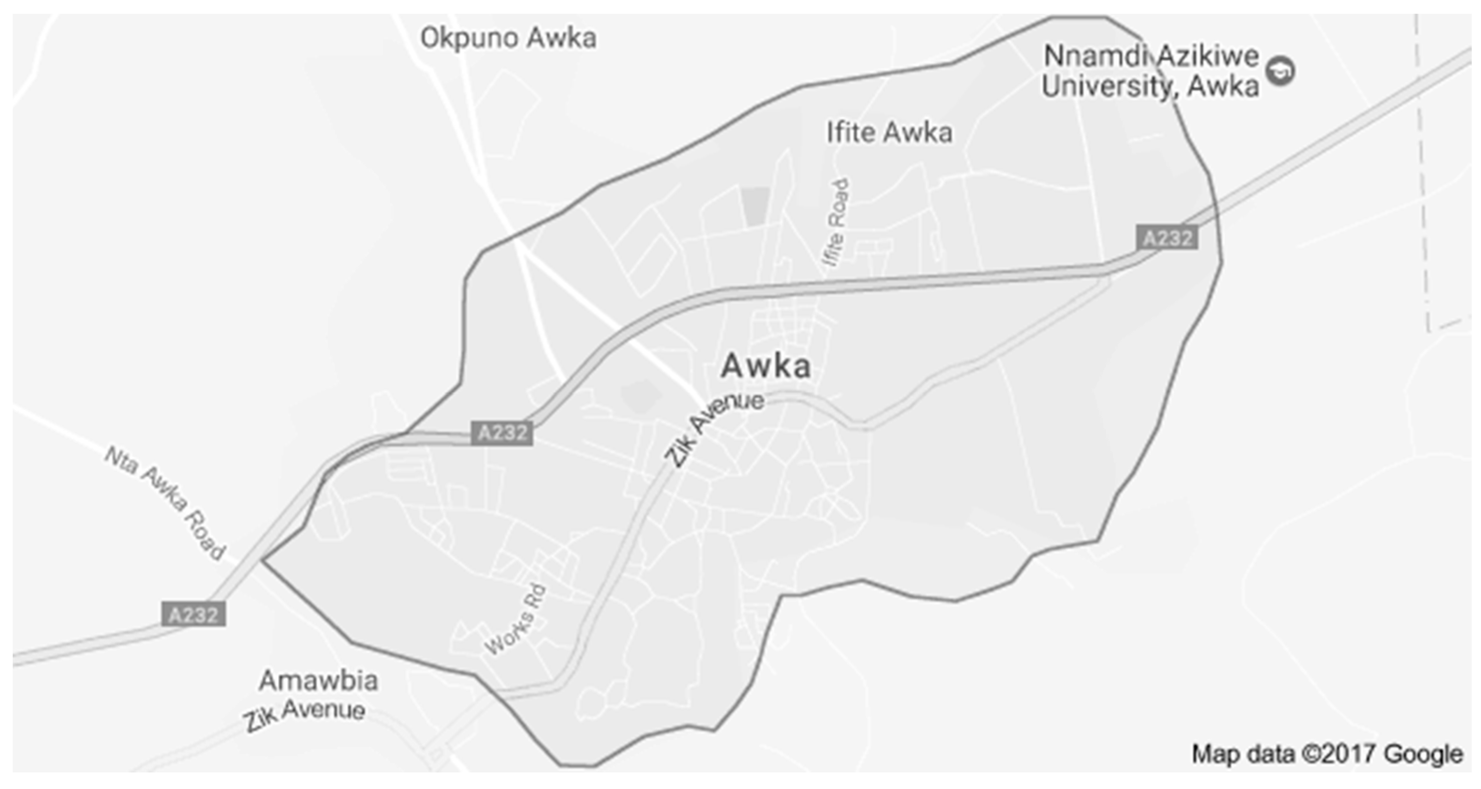
The low income areas are predominantly located to the left of the popular Nnamdi Azikiwe (Zik’s) avenue—the portion of Enugu to Onitsha old road that falls within the Awka metropolis (Figure 1). These areas predominantly have low cost accommodation, such as one room apartments with shared facilities and multiple room apartments also with shared facilities. It has unplanned housing patterns and poor infrastructure. Over time, lands were plotted, with little government supervision, in the near-right of the Nnamdi Azikiwe Avenue. Today, this area can be classified as the dwelling place for the majority of middle income class earners (civil servants, traders, etc.) who are predominantly non-indigenes. The major residential streets that fall within this area include Emma Nnaemeka, Works Road, Court Road, Kwata, Kenneth Dike, Umukabia, Araba, etc. This middle class area has moderate amenities like streets properly numbered. It also has several story buildings divided into flats.
The high income class are found in estates carefully plotted by government. They enjoy good facilities like tarred roads, good drainage system, more power supply, safe water supply, and better security. The houses are mostly bungalows, duplexes, and mansions. Udoka estate, Ngozika Estate, and Government Reserves Areas (GRAs) are the sub-areas under this class. In order to have a statistically balanced study, the study sample participants were drawn from the three income groupings.
3. Methodology
According to the year 2006 census, the number of regular households in Awka South local government area—as sourced from the national population commission Awka office—is 38,546, with a total population of 17,0723. The regular household is about 96.08% of all kinds of households in the area. Awka South is approximately the same as the municipality, called Awka, that constitutes the capital of Anambra state. Assuming a fixed household size (the ratio of population to household number or the number of occupants per household) of 17,0723/38,546 people per household and a fixed geometric population growth rate of r = 3.2% per annum (the national value) [1], the current number of households of the municipality is projected as;
which giveshouseholds.
Use is made of the simple sample size formula;
where N is the population size and e is the level of precision. In this study, and = 10%, giving the sample size of 100 households. Based on this sample size, 120 households were randomly drawn equally from the three major income areas to participate in the study; Udoka and Ngozika housing estates for high income earners, Umukabia, Works Road, and Kenneth Dike areas for middle income earners and Umudioka, Umubelele, and Amenyi for the low income residents. The judgment of income status was not just predicated by place of residence but was also confirmed with a questionnaire. The three major income groupings are not formally classified in Nigeria. They are classified here for quantitative reasons bearing in mind the current economic recession in Nigeria, which has drastically reduced purchasing power of households. They are as follows; (1) the low income stratum—this batch of households are considered to earn not more than ₦100,000, (2) the middle income stratum—this batch of households are considered to earn more than ₦100,000 but not more than ₦250,000, and (3) the high income stratum—this batch of households are considered to earn more than ₦250,000. This is shown in Table 1.
Ten days sampling was conducted. On the first day, numbered questionnaires were distributed to participants who were also numbered according to the questionnaires. The questionnaires were structured to extract the econo-demographic indices of the households. The reason for the research was explained to the participants and ethics of confidentiality guaranteed them. A waste bag was given to each participant. On the second day, the generated household waste and the questionnaires were gathered and taken to the study center. The mass and loose volume of the household waste, as collected, were measured first. The wastes were then sorted accordingly and the components weighed. The components of the wastes were re-mixed, compacted by human power, and the compact volume measured. The result for each participant were recorded on the logging table created on the correspondingly numbered questionnaire. The structure of the logging table is shown in Table 2. The procedure was repeated until 10-day data was sampled. Eighty two participants were consistent and their data were used in the analysis. This represents 11% level precision, which is only a slight deviation from the assumed 10%. The contributions of the economic strata in the sampled data are 36.6% from low income, 32.9% from middle income, and 30.5% from the high income. Therefore 82 by 10 sampled data sets were available for this study. This is large enough to justify assumption of normality, which is the foundation of regression analysis proposed in this work.
Composition of MSW is usually given in terms of descriptive statistics. This approach usually involves measures of location and central tendency (mostly mean), measures of dispersion (mostly standard deviation), and error or uncertainty. This tradition should be improved with mathematical and statistical tools. It proposed in this work that accuracy could be improved if composition of MSW is established through statistical regression analysis that minimizes the sum of square residuals. Zero-intercept first-order polynomial regression was suggested by Ozoegwu et al [18] for estimating biomass wastes generated in various stages of processing cassava into food. The fractions established through the method—for converting harvest data of cassava to waste biomass potential—were shown to be more accurate than fractions established through the descriptive approach. Since composition analysis of MSW is similar to estimation of the non-food biomass proportion of harvested cassava, it is believed that adaption of the zero-intercept first-order polynomial regression approach to MSW composition analysis will give better results. It must be noted that non-zero-intercept first-order multi-variate polynomial regression approach has been used to correlate MSW generation by households with socio-econo-demographic parameters like income, household size, education status, etc., as can be seen in the following works [19,20,21,22,23], but to the best of the knowledge of the authors, no work has applied regression to the composition analysis. Zero-intercept is imposed in regressive waste composition analysis to avoid the unrealistic cases of a non-zero constituent at zero waste generation. Similarly, zero-intercept is imposed in regressive waste per capita generation analysis to avoid the unrealistic case of non-zero per capita generation at zero household size. In the proposed zero-intercept first-order polynomial regression, the sampled waste generation is considered the independent variable, where the components (organic, plastic, metals, paper and textile, etc.) and volume (loose and compact volume) are considered dependent variables. Also, the daily per capita waste generations, the daily per capita constituent waste generations, and the daily per capita waste volumes are dependent on the household size in the proposed method.
The traditional descriptive approach is formulated for this study as follows. Suppose the total mass of waste generation of the th household () in th day () is represented as and the mass of the th component () for the day represented as , the descriptive approach gives the mean, standard deviation, and uncertainty of the composition as follows
It must be noted that in the descriptive approach, the elements of the sample, represented by a random variable , are assumed to be independently drawn from the population(s).
The proposed zero-intercept first-order polynomial regression approach is formulated for this study as follows. This approach to MSW composition analysis assumes that are the measured values of the random variable , which under deterministic conditions has a fixed value . The element is a component of a vector of dimension and the element is a component of a vector of dimension , such that
with the solution
where
The results from the two approaches— and , respectively, are compared in what follows, using the following statistical indices; the coefficient of determination R2, root mean square error (RMSE), mean bias error (MBE), mean absolute bias error (MABE), t-Test statistic, and correlation coefficient (r).
4. Results and Discussions
4.1. Sampling Results
The sampled results for the first day are presented graphically in Figure 2 below. The results are given on a per capita basis for mass in Figure 2a, volume in Figure 2b, and bulk density in Figure 2c. Statistically similar results are generated for the other 9 days. It is seen from Figure 2a that the compostable organic constituent of the total waste is the most visible amongst all the constituents.
4.2. Composition Analysis
Making use of equations (7–9), the organic composition is trained with 80% of the sampled data (days 1 to 4 and 6 to 9). The resulting organic composition or fraction in the generated waste is . Therefore the trained model correlating the organic composition with the total mass of MSW is
The statistics of the model are given in Table 3. It is seen from the table that the R2 = 0.79 is much higher than the value of 0.35 considered in [18] as the threshold for statistical correlation to be subsumed. This indicates success of the proposed approach. The model is statistically significant, as the calculated t-value of 1.2143 is less than the critical t-value of 2.201 at 95% confidence level. The RMSE, MBE, and MABE are small in comparison with the order of magnitude of . The correlation coefficient of r = 0.89 reflects strong positive correlation between the sampled and the predicted daily organic waste generation of households (DOWGH). Suppose the usual averaging method based on the equations (3–5) is used, the calculated mean of the organic composition together with the associated uncertainty is 0.7596 ± 0.0136 and the statistics associated with this value of composition are shown in Table 3. It is seen from t-Test values that statistical regression yields more statistically significant predictions than the averaging technique, under training. The remaining 20% of the sampled data (days 5 and 10) are used to test the model. In testing, the test sample data is statistically compared with the trained model. In essence, the capacity of the model to predict or extrapolate organic composition of an independently sampled MSW data is assessed. It is seen from Table 3 that the testing statistics are equally satisfactory. Also from t-Test values, it could be seen that statistical regression yields more statistically significant predictions than the averaging technique, under testing. The graphical depiction of results of training and testing are presented in Figure 3. It is seen from the graphs that though testing exhibited slightly superior statistics in Table 3, the testing data is actually less fitted (reflecting as slightly less slope and higher intercept; that is, more deviated from the ideal) than the training data.
The large percentage of organic waste, given by =%, is due to heavy dependence of typical Igbo families of the studied location on home-prepared, traditional foods. The organic composition of household waste of other Nigerian locations are 63.6% for Abuja [3] and 56.0% for Nsukka [5]. The comparatively high organic composition could be a reflection dwelling culture of Awka, which encourages walled-yard waste finding their way into waste bags rather than being swept into the surrounding bushes, or could be an effect of the current economic challenges in Nigeria. Economic recession could have reduced expenditure on magazines, newspapers, paper, foil packaged products, bottled water, canned, tinned, and bottled milk, sachet water, and many other processed products. Home-prepared food, being the most fundamental of needs, is not noticeably reduced in quantities, thus the associated waste features peels of tubers, leftover food, vegetable waste, cubs, shells, etc., more prominently in the waste composition. Albeit, this figure agrees closely with that found for several other popular Nigerian locations; 79.1% for Ogbomoso [6] and 79.0% for Lagos [23]. This organic composition compares to dumpsite organic composition of 73.7% of Uyo metropolis [15] (a southern Nigerian city). It must be noted that there is no basis to compare household and dumpsite organic waste compositions, as the latter includes the former together with other non-household MSW and suffers from scavenging and other factors. For comparison with other developing locations, the organic composition of household waste of 65.5% for Cape Haitian city in Haiti [24], 69.3% for Beijing in China [25], 65.5% for Suzhou in China [26], and 80.74% for Can Tho City in Vietnam [27] have been reported.
A similar regression analysis trains the plastic composition with 80% of the sampled data (days 1 to 4 and 6 to 9) to become . The statistics; R2 = 0.28, t-Test = 1.43, and r = 0.54 indicate poor (but adequate) significance of the correlation between the arising zero-intercept first-order model given as
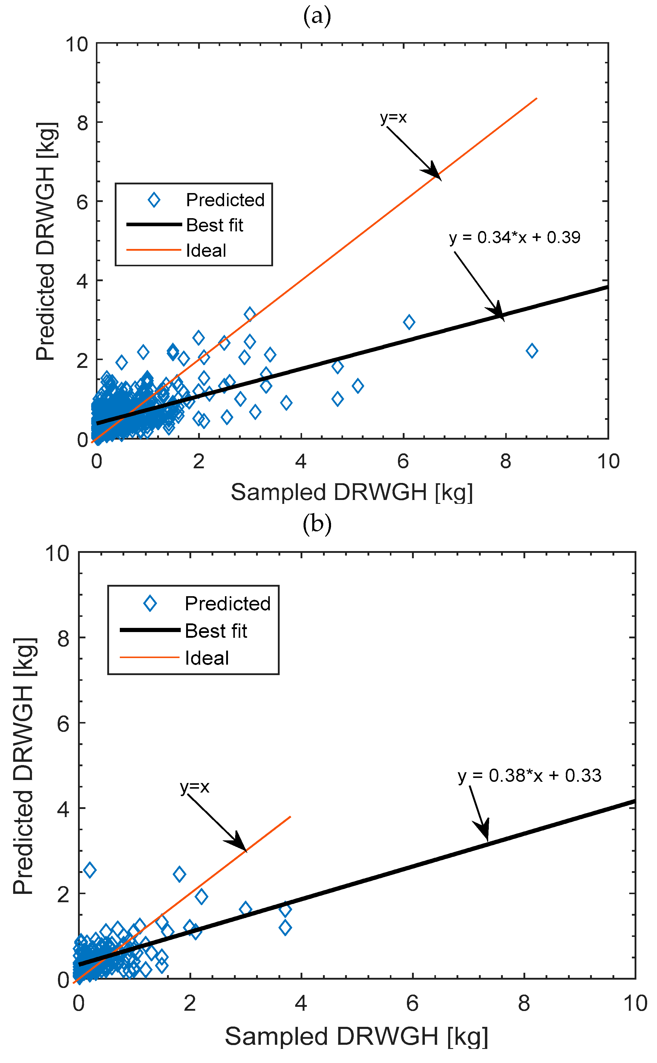
with the sampled data. This is because plastic-packaged food and drinks are far from being a basic component of household food mix, especially in this time of recession. Therefore, their appearance in household waste is extremely unpredictable. The same holds for metal and ceramics wastes. The percentage of plastic waste of 7.98% for the studied location, however, compares well with other Nigerian locations but with a reflection of expected recession-induced lower-fraction of overall waste; the percentage of plastic is 8.9% for Abuja [3] and 8.4% for Nsukka [5]. For comparison with other distant developing locations, the plastic composition of household waste for Beijing in China was 9.8% [25], for Can Tho City in Vietnam was 6.13% [27], for Tulsipur in Nepal was 10% [28], and for Cape Haitian city in Haiti was 9.2% [24]. The averaging technique gives with slightly less significant statistics relative to regression approach; R2 = 0.26, t-Test = 1.73, r = 0.54. On grouping the plastics, metal, and ceramic wastes together as recyclables (reusables are also implied), the extreme random effects are minimized and the results of the regressed and averaged models are shown in Table 4 and Figure 4; the averaging method performed slightly better this time. Though the organic composition model exhibits much higher statistical significance, the model for recyclables met the basic requirements for statistical correlation to be subsumed. In comparing Figure 3 and Figure 4, it is seen that the organic composition varies over a wider domain than the recyclable composition. This could be an indication that the former varies more deterministically with household socio-econo-demographic parameters than the latter in the studied location and during the study time. This is reasonable as traditional food, from which organic composition derives, is a much more fundamental need than the plastic packed items.
4.3. Volume and Bulk Density Analysis
Spatial volume is an important parameter in MSW management. The volume of solid wastes, as collected from households, is called loose volume (LV). Normally, space is saved for more portable evacuation by compacting the waste to minimize transportation cost. After the LV was measured in a calibrated bin, the waste was sorted to allow measurement of component masses. Thereafter, the components were mixed again in the bin and pressed down by human muscle power and the compact volume (CV) was recorded. Statistical regression, as done above, is used to establish factors for converting household MSW generation to LV and CV. The models and the statistics are shown in Table 5, while the graphical analysis is shown in Figure 5. It is seen that the factor for conversion of mass of household MSW to LV is L/kg, while that for conversion to CV is L/kg. The statistics indicate acceptable levels of correlation of predicted and sampled LV and CV from the standpoints of coefficients of determination and correlation. The compaction ratio, given as , becomes . It must be noted that can, alternatively, be established via regression that considers LV as the regressor and CV as the response. Doing this gives = 0.5050, with the statistics R2 = 0.7423, t-value = 1.9895, and r = 0.8645, which indicate significant statistical correlation between LV and CV. The procedure can be repeated when a standard evacuation truck is used, which obviously will exert a higher compaction ratio. However, waste evacuation by entrepreneurs who hire manual laborers to load and compact the waste is widespread in Nigeria. Thus, the calculated compaction ratio of 0.5050 will be in the range they may need in planning and this translates to saying that little above half of loose volume is needed for compact evacuation. The loose and compact bulk densities are the reciprocals of and , therefore loose bulk density is kgm−3, while the compact kgm−3. The calculated loose bulk density is in the range 250 to 500 kg/m3, reported for low income countries by [29].
4.4. Per Capita Waste Generation
The daily per capita waste generation is obtained by regression that considers household size as the regressor and daily solid waste generation () as the response, where “I” designates any of total, organic, recyclable, and plastic and textile wastes. The daily per capita total waste generation (), daily per capita organic waste generation (), daily per capita recyclable waste generation (), and daily per capita paper and textile waste generation () are generated as coefficients of in the models in Table 6. The t-test indicates significant statistical relation between the sampled and predicted masses. It must be noted that statistical regression performs better than the averaging approach, as seen from the column for total per capita waste generation, indicating that overall—even in the case of below-adequate statistical significance—the proposed zero-intercept first-order polynomial regression method is more reliable for composition analysis than the traditional averaging method. From the table = kg/capita/day, = kg/capita/day, kg/capita/day, and kg/capita/day. The daily per capita total solid waste generation of kg/capita/day (from regression) or kg/capita/day (from averaging) is lower than the value reported for the capital city of Nigeria, Abuja with = 0.54 kg/capita/day [4] and subsequently = 0.634 kg/capita/day [3]. Awka is the capital of Anambra state, which can compete as the state with the most economically empowered citizenry in Nigeria. Therefore economic parameters—known to influence solid waste generation [25]—cannot explain the low daily per capita total solid waste generation. The most cogent explanation could be the subsisting severe economic recession which has drastically reduced the purchasing power of Nigerians during the time of sampling. This is an indication that under the economic crunch, Nigeria may have relapsed to low-income status that has been characterized by [23], with 0.4 kg/capita/day 0.6 kg/capita/day. The middle income countries are characterized with 0.5 kg/capita/day 0.9 kg/capita/day [3], explaining the high value of 0.634 kg/capita/day for reported in the study [3]—a work carried before the recession when Nigeria could be regarded as middle income. It is curious to note the = kg/capita/day value for Awka, as found in this work, is much higher than the kg/capita/day for Ogbomoso reported in [6].
The daily per capita LV of generated solid waste is obtained by regression that considers household population as the regressor and sampled daily LV of household solid waste generation as target response. This is also done for CV. The daily per capita LV of generated solid waste is = 0.9021dm−3/capita/day (R2 = −0.1150, t-Test = 3.8778, and r = 0.2229) and the daily per capita CV of generated solid waste is = 0.4508dm−3/capita/day (R2 = −0.0157, t-Test = 2.6265, and r = 0.2320). Statistical significance is rejected and the averaging technique is used to calculate the parameters as follows: = 1.0767dm−3/capita/day ±2.15% (R2 = −0.2267, t-Test = 4.4803, and r = 0.2229) and = 0.5287dm−3/capita/day ±2.67% (R2 = −0.0718, t-Test = 3.6156, and r = 0.2320). It must be noted that though the uncertainty in the averaging method is low, its prediction of LV of household daily solid waste generation is less statistically correlated with the sampled data than the regression approach, thus = 0.9021dm−3/capita/day and = 0.4508dm−3/capita/day are adopted as the results of this work. This goes to say that the zero-intercept linear regression approach, introduced here, is more often than not superior in predictive reliability than the usual averaging approach.
4.5. Patterns across the Income Groups
Using the proposed method, the MSW composition of the study area is characterized by the major economic income groups; low income, middle income, and high income. The statistics are summarized in Table 7. From Table 8 it is seen that the trends of organic composition (), recyclable composition (), and per capita waste generation (), across the income groups, follow known results; organic composition is highest in the low income group, followed by the middle income group and then the high income group. The per capita waste generation is lowest in the low income group, followed by the middle income group and then the high income group. The loose volume of per capita waste generation () is highest in the middle income group, followed by the high income group and then the low income group. The same is true for the compact volume of per capita waste generation (). For having the highest , the high income status should be expected to require the highest volume or space for the generated waste on per capita basis. The reason for this anomaly could be that, on a per capita basis, the middle income earners generate more hollow and space consuming wastes in the study area. The most likely culprit should be plastics (bottles, bags) and paper and textiles, thus the middle income earners may have generated more of these on a per capita basis. This is actually the case, as they generated 46.3 ± 3.0 g/capita/day of plastic while the high income group generated 43.5 ± 2.7 g/capita/day and the low income group generated 31.7 ± 2.2 g/capita/day. This is also the case, as the middle income group generated 33.5 ± 3.1 g/capita/day of paper/textile, while high income group generated 30.7 ± 3.3 g/capita/day and low income group generated 21.5 ± 1.9 g/capita/day. This could be due to occupational variation amongst the groups; the middle income earners tended to be predominantly civil servants (teachers, lecturers, etc.) that produce paper wastes.
5. The City-Wide Waste Generation
The daily per capita quantities established in the foregoing section are used to calculate the daily city-wide quantities. Such city-wide estimates are necessary for resource and capital allocation to MSW management. The daily per capita quantities of interest are those that jointly cover for the three income groups and relate to the overall management. They are = kg/capita/day, = kg/capita/day, kg/capita/day, kg/capita/day, = 0.9021 dm−3/capita/day, and = 0.4508dm−3/capita/day. Adopting a population of 17,0723 (according to the year 2006 census) and assuming a fixed geometric population growth rate of r = 3.2% per annum (the national value) [1], the projected population for a future year “20XY” is households. Since only households were sampled, correction factors are needed to transform results to overall generation capacity of Awka. Household waste is about 40–60% of urban waste [3]. The survey by [2] showed that 82% of the solid waste generated in a rapidly growing urban area in Central Nigeria came from households. Since Awka is not an industrial area, it is assumed that household contribution to the MSW is in the high side of the known range for Nigerian locations, therefore, 75% of MSW is assumed to come from households. The Awka city-wide generation for the year 2016 becomes
where = or and = , , , , , or . Therefore, the daily total MSW generation is 130.0348 tonne/day, the daily compostable MSW generation is 95.7872 tonne/day, the daily recyclable MSW generation is 25.8884 tonne/day, the daily paper and textile MSW generation is 7.8601 tonne/day, the daily loose volume of MSW is 281.3730 m3/day, and the daily compact volume of MSW is 140.6085 m3/day. These data would aid managers in allocation of resources to the city waste management. For example, given the capacity of evacuation trucks, the needed number of trucks can be recommended to depend on the number of through puts allowed for complete evacuation.
6. Conclusions
Municipal solid waste (MSW) generation is enormous and grossly under-characterized in Nigeria. Also, there exists a necessity for an efficient management scheme that would allocate the biomass component of the MSW as renewable energy feedstock and also exploit the recyclables and reusables. For these reasons, waste generated in a previously not-studied location—Awka municipality—was sampled and characterized, resulting in an enhanced data bank for MSW management in Nigeria. The characterization was done with improved accuracy using a new method called zero-intercept first-order polynomial regression. Eighty percent of the 820 by 11 data matrix -extracted from a ten-day sampling process—was used in model training, while the remaining twenty percent was used in model testing. The testing statistics agree closely with those of training, indicating the predictive capacity of the approach. The results from the new approach significantly demonstrated improved accuracy relative to the traditional averaging technique. Furthermore, relying on the over-stressed adverse impact of poorly managed waste on public health, waste management has become a key performance indicator of sustainable development. Therefore, the relevance of the current study comes to bare, as it pointed needs for city waste authorities to work with more accurate information in order to ensure optimal allocation of resources and to provide satisfactory services to the society. The results of the waste composition from current studies readily indicate large proportions of organic waste. This is an opportunity that could be seized to produce compost for the city’s agrarian base. Substantial revenue could also be generated from the high quantity of recyclables found in the study through establishing a material recovery facility managed by the Awka municipal council.
Author Contributions
Conceptualization: O.B.E.; Methodology: O.B.E., C.N.M. and C.G.O. Formal analysis: C.G.O. and O.B.E.; Data curation: O.B.E.; Writing original draft preparation: O.B.E. and C.G.O.; Review and editing: O.B.E. and C.N.M.; Supervision, C.N.M.; Project administration, C.N.M.
Funding
This research received no external funding.
Acknowledgments
We are grateful to staff of National Population Commission, Awka office for their help during data collection. We also thank the anonymous reviewers for their constructive criticism towards improving the quality of the manuscript.
Conflicts of Interest
The authors declare no conflict of interest.
References
- Population Reference Bureau. 2013 World Population Data Sheet, 2013. Available online: www.unfpa.org (accessed on 7 September 2017).
- Sha’Ato, R.; Aboho, S.Y.; Oketunde, F.O.; Eneji, I.S.; Unazi, G.; Agwa, S. Survey of solid waste generation and composition in a rapidly growing urban area in Central Nigeria. Waste Manag. 2007, 27, 352–358. [Google Scholar] [CrossRef] [PubMed]
- Ogwueleka, T.C. Survey of household waste composition and quantities in Abuja, Nigeria. Resour. Conserv. Recy. 2013, 77, 52–60. [Google Scholar] [CrossRef]
- Imam, A.; Mohammed, B.; Wilson, D.C.; Cheeseman, C.R. Solid waste management in Abuja, Nigeria. Waste Manag. 2008, 28, 468–472. [Google Scholar] [CrossRef] [PubMed]
- Ogwueleka, T.C. Analysis of urban solid waste in Nsukka: Nigeria. J. Solid Waste Technology Manag. 2003, 4, 239–246. [Google Scholar]
- Afon, A. An analysis of solid waste generation in a traditional African city: the example of Ogbomoso, Nigeria. Environ. Urban 2007, 19, 527–537. [Google Scholar]
- Palanivel, T.M.; Sulaiman, H. Generation and Composition of Municipal Solid Waste (MSW) in Muscat, Sultanate of Oman. APCBEE Procedia 2014, 10, 96–102. [Google Scholar] [CrossRef] [Green Version]
- Ozoegwu, C.G.; Mgbemene, C.A.; Ozor, P.A. The status of solar energy integration and policy in Nigeria. Renew. Sust. Energy Rev. 2017, 70, 457–471. [Google Scholar] [CrossRef]
- Scarlet, N.; Motola, V.; Dallemand, J.F.; Monforti-Ferrario, F.; Mofor, L. Evaluation of energy potential of Municipal Solid Waste from African urban areas. Renew. Sust. Energy Rev. 2015, 50, 1269–1286. [Google Scholar] [CrossRef] [Green Version]
- Hoornweg, D.; Bhada-Tata, P. What a Waste, A Global Review of Solid Waste Management; The urban Development Series Knowledge papers; The World Bank: Washington, DC, USA, 2012. [Google Scholar]
- Moya, M.; Aldas, C.; Lopez, G.; Kaparaju, P. Municipal solid waste as a valuable renewable energy resources: a worldwide opportunity of energy recovery by using Waste-To-Energy Technologies. Energy Procedia 2017, 134, 286–295. [Google Scholar] [CrossRef]
- ISWA. ISWA Waste-to-Energy State-of-the-Art- Report; International Solid Waste Association: Copenhagen, Denmark, 2012; p. 201. [Google Scholar]
- McDougall, F.; White, P.; Franke, M.; Hindle, P. Integrated Solid Waste Management: A Life-Cycle Inventory; Blackwell: Oxford, UK, 2001. [Google Scholar]
- Agunwamba, J.C. Analysis of scavengers’ activities and recycling in some cities of Nigeria. Environ. Manag. 2003, 32, 116–127. [Google Scholar] [CrossRef]
- John, N.M.; Edem, S.O.; Ndaeyo, N.U.; Ndon, B.A. Physical Composition of Municipal Solid Waste and Nutrient Contents of Its Organic Component in Uyo Municipality, Nigeria. J. Plant Nutr. 2006, 29, 189–194. [Google Scholar] [CrossRef]
- Agunwamba, J.C. Solid waste management in Nigeria: problems and issues. Environ. Manag. 1998, 22, 849–856. [Google Scholar] [CrossRef] [PubMed]
- Federal Ministry of Environment. Blueprint on municipal solid waste management in Nigeria, Abuja, Nigeria; Federal Ministry of Environment: Abuja, Nigeria, 2000. [Google Scholar]
- Ozoegwu, C.G.; Eze, C.; Onwosi, C.O.; Mgbemene, C.A.; Ozor, P.A. Biomass and bioenergy potential of cassava waste in Nigeria: estimations based partly on rural-level garri processing case studies. Renew Sust. Energy Rev. 2017, 72, 625–638. [Google Scholar] [CrossRef]
- Ojeda-Benítez, S.; Vega, C.A.; Marquez-Montenegro, M.Y. Household solid waste characterization by family socioeconomic profile as unit of analysis. Resour. Conserva. Recy. 2008, 52, 992–999. [Google Scholar] [CrossRef]
- Thanh, N.P.; Matsui, Y.; Fujiwara, T. Household solid waste generation and characteristic in a Mekong Delta city: Vietnam. J. Environ. Manag. 2010, 91, 2307–2321. [Google Scholar] [CrossRef] [PubMed]
- Gua, B.; Wanga, H.; Chen, Z.; Jiang, S.; Zhu, W.; Liu, M.; Chen, Y.; Wua, Y.; Heb, S.; Cheng, R.; Yang, J.; Bi, J. Characterization, quantification and management of household solid waste: A case study in China. Resour. Conserv. Recy. 2015, 98, 67–75. [Google Scholar] [CrossRef]
- Mendenhall, W. Statistics for Administrators; Iberoamericana: S.A. de C.V., México, 1990. [Google Scholar]
- Cointreau, S.J. Environmental Management of Urban Solid Waste in Developing Countries: A Project Guide; Urban Development Technical Paper No. 5; World Bank: Washington, DC, USA, 1982. [Google Scholar]
- Philippe, F.; Culot, M. Household solid waste generation and characteristics in Cape Haitian city, Republic of Haiti. Resour. Conserv. Recy. 2009, 54, 73–78. [Google Scholar] [CrossRef]
- Qu, X.; Li, Z.; Xie, X.; Sui, Y.; Yang, L.; Chen, Y. Survey of composition and generation rate of household wastes in Beijing, China. Waste Manag. 2009, 29, 2618–2624. [Google Scholar] [CrossRef]
- Thanh, N.P.; Matsui, Y.; Fujiwara, T. Assessment of plastic waste generation and its potential recycling of household solid waste in Can Tho City, Vietnam. Environ. Monit. Assess. 2011, 175, 23–35. [Google Scholar] [CrossRef]
- Dangia, M.B.; Urynowicz, M.A.; Belbase, S. Characterization, generation, and management of household solid waste in Tulsipur, Nepal. Habitat Int. 2013, 40, 65–72. [Google Scholar] [CrossRef] [Green Version]
- Holmes, J.R. Managing Solid Wastes in Developing Countries; John Wiley Sons: Chichester, UK, 1984; p. 312. [Google Scholar]
- Mancini, S.; Nogueira, A.; Kagohara, D.; Schwartzman, A.; Mattos, T. Recycling potential of urban solid waste destined for sanitary landfills: the case of Indaiatuba, SP, Brazil. Waste Manag. Res. 2007, 25, 517–523. [Google Scholar] [CrossRef] [PubMed]
Figure 1.
Showing the location of popular Nnamdi Azikiwe (Zik’s) Avenue.

Figure 2.
Results of first day sampling. (a) Mass of the total and constituent wastes, (b) loose and compact volume, and (c) bulk densities for loose and compact wastes. Statistically similar results are generated for the other 9 days.
Figure 2.
Results of first day sampling. (a) Mass of the total and constituent wastes, (b) loose and compact volume, and (c) bulk densities for loose and compact wastes. Statistically similar results are generated for the other 9 days.
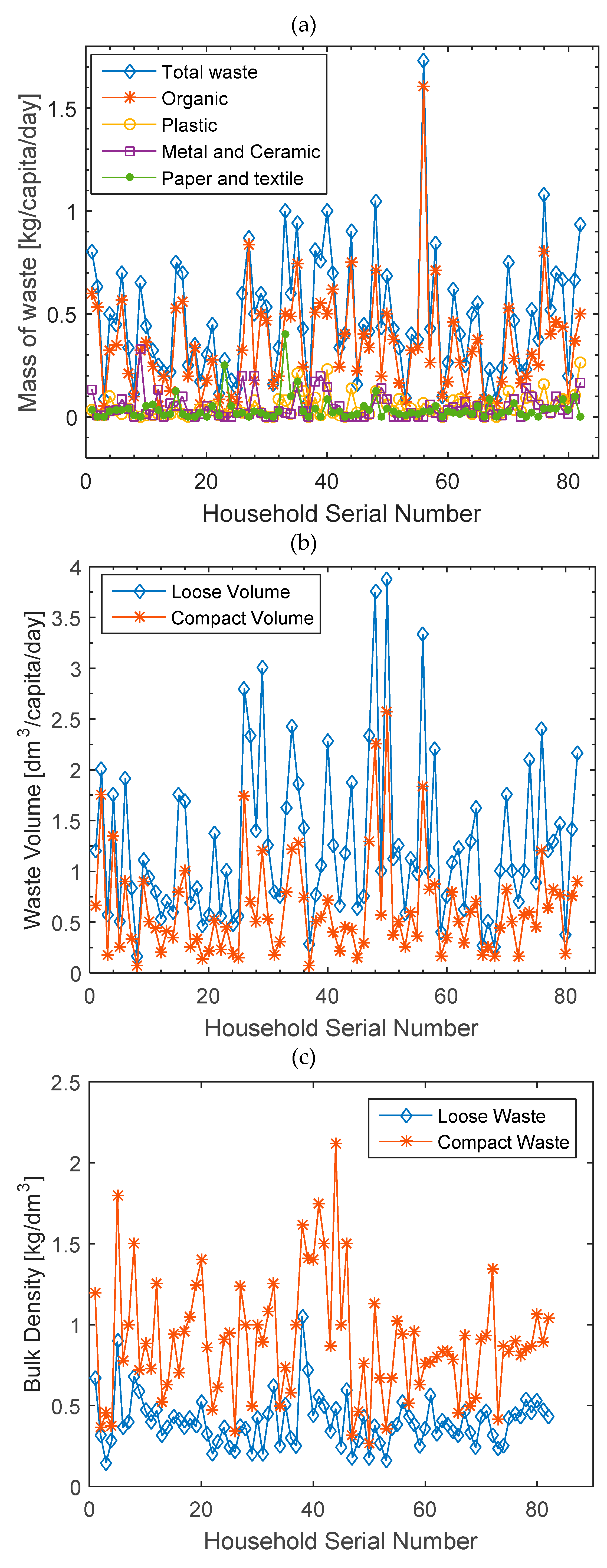
Figure 3.
The graphical depiction of results of training (a) and testing (b) for organic composition. The testing is only slightly less fitted (reflecting as slightly less slope and higher intercept, that is, more deviated from the ideal) than the training. DOWGH means Daily Organic Waste Generated from Household.
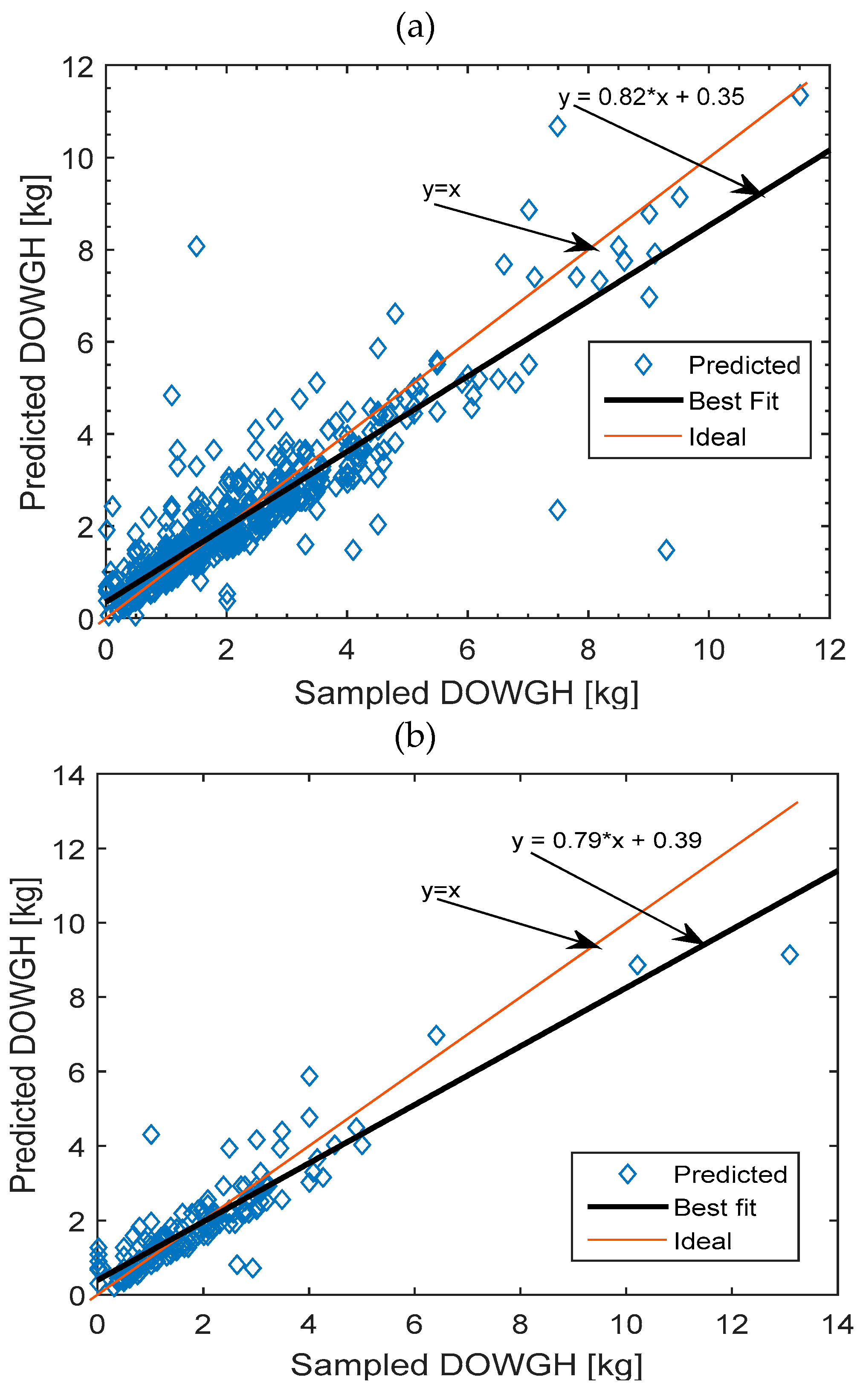
Figure 4.
The graphical depiction of results of training and testing for recyclable composition. (a) Training and (b) testing. DRWGH means Daily Recyclable Waste Generated from Households.
Figure 4.
The graphical depiction of results of training and testing for recyclable composition. (a) Training and (b) testing. DRWGH means Daily Recyclable Waste Generated from Households.

Figure 5.
The graphical depiction of results of volume analysis. (a) loose volume and (b) compact volume. LVDWGH and CVDWGH means Loose Volume or Compact Volume of Daily Waste Generated from Households.
Figure 5.
The graphical depiction of results of volume analysis. (a) loose volume and (b) compact volume. LVDWGH and CVDWGH means Loose Volume or Compact Volume of Daily Waste Generated from Households.


Table 1.
The income Stratum and Location.
| Income Stratum | Earning Range (Naira) | Location Areas |
|---|---|---|
| Low-income | >or = 100,000 | Umudioka, Umubele, Amenyi |
| Middle-income | >100,000 < or = 250,000 | Umukabia, Works Rd, Kenneth Dike |
| High-Income | >250,000 | Udoka, Ngozika |
Table 2.
The structure of the logging table for waste analysis.
| SN | Tm (kg) | Lv (l) | Plastic (kg) | Met/cera (kg) | Orga (kg) | Pap/tex (kg) | LignoC (kg) | Pres vol (l) | Others | Income Status × 10 −3 | House Popu. |
|---|---|---|---|---|---|---|---|---|---|---|---|
| 1 | 12.0 | 18.0 | 0.5 | 2.0 | 9.0 | 0.5 | 0 | 10.0 | 0 | >250 | 15 |
| 82 | 2.0 | 7.0 | 0.4 | 0.1 | 1.2 | 0.1 | 0.1 | 5.4 | 0.1 | 100 &150 | 4 |
Table 3.
The statistical indices of the regression and averaged models of organic MSW composition.
| Statistical Index | Training | Testing | ||
|---|---|---|---|---|
| Statistical Regression | Averaging | Statistical Regression | Averaging | |
| Model | ||||
| R2 | 0.7889 | 0.7855 | 0.82 | 0.8206 |
| RMSE | 0.7355 | 0.7415 | 0.6868 | 0.6857 |
| MBE | −0.0349 | 0.0412 | −0.018 | 0.0517 |
| MABE | 0.4281 | 0.4229 | 0.4444 | 0.4378 |
| t-Test | 1.2143 | 1.4232 | 0.3343 | 0.9654 |
| R | 0.889 | 0.889 | 0.9065 | 0.9065 |
Table 4.
The statistical indices of the regression and averaged models of recyclable MSW composition.
Table 4.
The statistical indices of the regression and averaged models of recyclable MSW composition.
| Statistical Index | Training | Testing | ||
|---|---|---|---|---|
| Statistical Regression | Averaging | Statistical Regression | Averaging | |
| Model | ||||
| R2 | 0.3794 | 0.3722 | 0.3506 | 0.3540 |
| RMSE | 0.5777 | 0.5811 | 0.4862 | 0.4849 |
| MBE | 0.0346 | −0.0159 | 0.0277 | −0.0185 |
| MABE | 0.3465 | 0.3356 | 0.3226 | 0.3146 |
| t-Test | 1.5345 | 0.6995 | 0.7289 | 0.4882 |
| R | 0.6212 | 0.6212 | 0.5958 | 0.5958 |
Table 5.
The statistical indices of the predicted loose and compact volume of daily waste generation of households.
Table 5.
The statistical indices of the predicted loose and compact volume of daily waste generation of households.
| Statistical Index | LV | CV |
|---|---|---|
| Model | ||
| R2 | 0.4083 | 0.3674 |
| RMSE | 0.0027 | 0.0018 |
| MBE | −0.0009 | −0.0004 |
| MABE | 0.0019 | 0.0011 |
| t-Test | 9.4543 | 5.7534 |
| R | 0.7605 | 0.6627 |
Table 6.
The statistical indices of the regression and averaged models of per capita household MSW.
| Statistical Index | Total Per Capita Waste | Organic Per Capita Waste | Recyclable Per Capita Waste | Plastic and Textile | |
|---|---|---|---|---|---|
| Statistical Regression | Averaging | Statistical Regression | Statistical Regression | ||
| Model | |||||
| R2 | 0.1121 | 0.0896 | 0.0613 | 0.0851 | 0.0128 |
| RMSE | 1.8785 | 1.9022 | 1.5563 | 0.6786 | 0.2734 |
| MBE | −0.0997 | 0.1808 | −0.0938 | 0.0035 | −0.0080 |
| MABE | 1.3819 | 1.4438 | 1.1544 | 0.4264 | 0.1610 |
| t-Test | 1.5209 | 2.7329 | 1.7284 | 0.1485 | 0.8360 |
| R | 0.3641 | 0.3641 | 0.2988 | 0.2921 | 0.1403 |
Table 7.
The statistics for the three income groupings.
| Low-Income | Middle-Income | High-Income | |||||||
|---|---|---|---|---|---|---|---|---|---|
| R2 | t-Test | R | R2 | t-Test | R | R2 | t-Test | R | |
| r(org) | 0.8511 | 0.2376 | 0.9226 | 0.8732 | 1.0815 | 0.9356 | 0.7312 | 0.6377 | 0.8559 |
| r(recyc) | 0.2075 | 0.1169 | 0.4556 | 0.2176 | 1.2658 | 0.4847 | 0.3974 | 0.6391 | 0.6327 |
| M(tm) | −0.3702 | 2.8343 | −0.0882 | −0.2063 | 1.9226 | 0.0119 | 0.1685 | 0.3863 | 0.4161 |
| V(lv) | −0.3554 | 2.7738 | −0.0553 | 0.2124 | 1.9509 | 0.0340 | −0.0385 | 1.8607 | 0.3066 |
| V(cv) | −0.1819 | 2.1078 | −0.0223 | −0.1366 | 1.6086 | 0.0108 | 0.1176 | 0.9569 | 0.3843 |
| r(comp) | 0.7337 | 1.7231 | 0.8629 | 0.7183 | 1.0944 | 0.8506 | 0.7240 | 0.3694 | 0.8513 |
Table 8.
Composition of study area household MSW by income groups.
| Low Income | Middle Income | High Income | |
|---|---|---|---|
| 0.7904 | 0.7403 | 0.7144 | |
| 0.1527 | 0.1698 | 0.2304 | |
| [kg/capita/day] | 0.30 | 0.45 | 0.49 |
| [dm−3/capita/day] | 0.75 | 1.08 | 0.96 |
| = [dm−3/capita/day] | 0.35 | 0.53 | 0.50 |
| 0.4913 | 0.5028 | 0.5122 | |
| [kg/m3] | 444.4 | 449.5 | 575.9 |
| [kg/m3] | 936.4 | 901.4 | 1102.1 |
© 2019 by the authors. Licensee MDPI, Basel, Switzerland. This article is an open access article distributed under the terms and conditions of the Creative Commons Attribution (CC BY) license (http://creativecommons.org/licenses/by/4.0/).
Share and Cite
MDPI and ACS Style
Ezeudu, O.B.; Ozoegwu, C.G.; Madu, C.N. A Statistical Regression Method for Characterization of Household Solid Waste: A Case Study of Awka Municipality in Nigeria. Recycling 2019, 4, 1. https://doi.org/10.3390/recycling4010001
AMA Style
Ezeudu OB, Ozoegwu CG, Madu CN. A Statistical Regression Method for Characterization of Household Solid Waste: A Case Study of Awka Municipality in Nigeria. Recycling. 2019; 4(1):1. https://doi.org/10.3390/recycling4010001
Chicago/Turabian StyleEzeudu, Obiora B., Chigbogu G. Ozoegwu, and Christian N. Madu. 2019. "A Statistical Regression Method for Characterization of Household Solid Waste: A Case Study of Awka Municipality in Nigeria" Recycling 4, no. 1: 1. https://doi.org/10.3390/recycling4010001