
An Experimental Study of the Aeroacoustic Properties of a Propeller in Energy Harvesting Configuration
by
 , , , and
Paolo Candeloro
1,* ,
,
Edoardo Martellini
1,
Robert Nederlof
2,
Tomas Sinnige
2 and
Tiziano Pagliaroli
1,* 1
Engineering Department, Universitá degli studi Niccoló Cusano, Via Don Carlo Gnocchi 3, 00166 Rome, Italy
2
Flow Physics and Technology Department, Faculty of Aerospace Engineering, Delft University of Technology, Kluyverweg 1, 2629 HS Delft, The Netherlands
*
Authors to whom correspondence should be addressed.
Fluids 2022, 7(7), 217; https://doi.org/10.3390/fluids7070217
Submission received: 13 April 2022
/
Revised: 17 June 2022
/
Accepted: 22 June 2022
/
Published: 27 June 2022
(This article belongs to the Special Issue Recent Advances in Aerodynamics and Aeroacoustics: Towards Greener Aviation)
Abstract
:The aim of the present manuscript is to investigate the noise footprint of an isolated propeller in different flight configurations for the propulsion of a hybrid-electric aircraft. Experimental tests were performed at the Low-Turbulence Tunnel located at Delft University of Technology with a powered propeller model and flush-mounted microphones in the tunnel floor. The propeller was investigated at different advance ratios in order to study the noise impact in propulsive and energy harvesting configurations. For brevity, this work only reports the results at the conditions of maximum efficiency in both propulsive and energy harvesting regimes, for a fixed blade pitch setting. Comparing these two configurations, a frequency-domain analysis reveals a significant modification in the nature of the noise source. In the propulsive configuration, most of the energy is related to the tonal noise component, as expected for an isolated propeller; however, in energy harvesting configuration, the broadband noise component increases significantly compared to the propulsive mode. A more detailed analysis requires separation of the two noise components and, for this purpose, an innovative decomposition strategy based on proper orthogonal decomposition (POD) has been defined. This novel technique shows promising results; both in the time and in the Fourier domains the two reconstructed components perfectly describe the original signal and no phase delays or other mathematical artifices are introduced. In this sense, it can represent a very powerful tool to identify noise sources and, at the same time, to define a proper control strategy aimed at noise mitigation.
1. Introduction
In recent years, the urgency of reducing humans’ environmental impact has led to an awareness of countries and their governments. For this purpose, NASA has pointed out strict constraints for energy consumption, nitrogen oxides () and noise for three generations of aeroplanes [1,2]. Moreover, the International Civil Aviation Organization (ICAO) set certification standards for noise and emissions in 2020 [3]. In this scenario, aircraft concepts involving electric propulsion (EP) have become of great public interest [4], because through electrification, a strong reduction of aircraft environmental impact can be achieved. Among the many solutions for aircraft design opened by EP, one of the most interesting and well-studied is distributed electric propulsion (DEP). The key idea behind distributed propulsion is to spread the propulsive elements over the airframe [5]. DEP has the potential to drastically reduce the take-off noise, fuel consumption and emission levels for the lighter aircraft sector [5,6]. In addition to advanced propulsion integration, EP enables energy harvesting solutions. Specifically, during part of the mission that does not require power input, electric engines can be used as generators, resulting in energy recovery during flight that will impact the total mission energy, especially when aiming for steep descent trajectories. In particular, one way to harvest energy is to use the propellers as airborne wind turbines in specific parts of the flight mission, as in the present study. In this approach, the blade sections will operate at negative angles of attack, resulting in an inversion of the direction of the aerodynamic forces. This results in the generation of a negative torque that can be converted into electrical energy by the motor. The idea of using propellers to recover energy has already been proposed for gliders and ships [7,8,9,10,11], and also for turbofan engines [12,13]. These studies confirm that it is possible to employ rotors to recover energy in windmilling conditions by considering the reversed direction of the aerodynamic forces and moments (due to the shift to negative angles of attack on the blade section), necessary for the harvesting of energy. Furthermore, the use of propellers to recover energy has been explored in the literature, for example in Cherubini et al. [14]. More recently, Erzen et al. [15] displayed the potential of using propellers to recover energy for an electric aircraft.
Even though the scientific community has shown great interest in the use of propellers to recover energy, little attention has been given to the study of noise generated in these unconventional operating conditions. In an energy harvesting configuration, increased separation of the blades is expected compared to the conventional propulsion configuration [16], which may lead to stronger broadband noise emissions. These issues suggest that common noise reduction strategies, useful for the propulsive mode, may not be equally effective in the event of a shift to such a usage regime.
In propeller-driven aircraft, the main noise sources are the engine and the propeller itself [17]. The noise radiated by propellers has been described in detail in the literature [18,19,20,21,22].
Generally, the propeller aerodynamic noise is divided into narrow- and broadband components [18,23,24,25]:
where is the narrowband (or tonal) component of pressure fluctuations, whereas is the broadband counterpart.
For thin blades operating at subsonic Mach numbers (), the narrowband contribution is given by the sum of two main sources:
where denotes the pressure fluctuations related to blade thickness while is related to aerodynamic loading. The thickness term accounts for the fluid displacement due to the body, while the loading component takes account of the force distribution over the body surface.
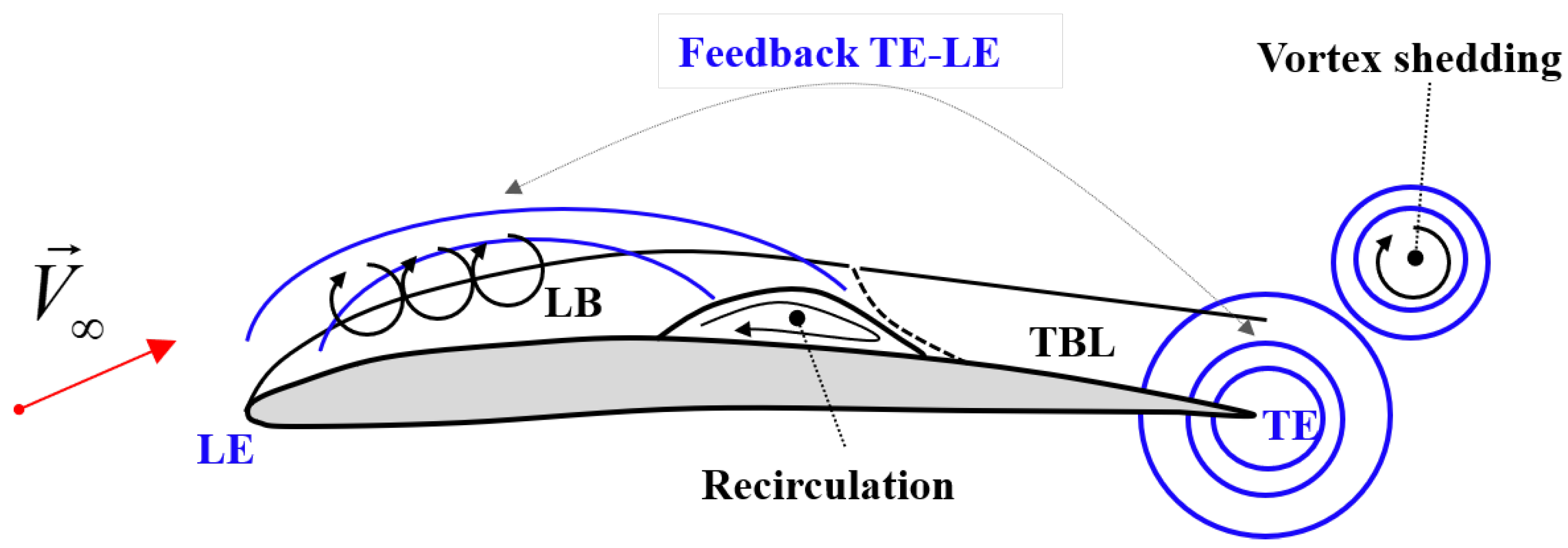
However, propeller broadband noise is related to the interaction of turbulent flow structures with the blade edge and to flow separation. Generally, the broadband contribution can be split as:
where is the trailing edge component related to the interaction of the turbulent boundary layer over the blade surface, is the leading edge component related to the incoming flow and is the separation term. A schematic representation of the main broadband noise sources involved is presented in the Figure 1.
Propeller sound emissions provide a great challenge to the task of noise characterization and prediction. Indeed, the main noise sources remain consistent with those associated with helicopters. In the case presented in this work there are numerous unknowns to be investigated, such as the effect of reduced size or the balance between tonal noise and broadband noise [26].
In the study of rotor noise, there is great interest in the definition of advanced analysis tools, in particular for the decomposition of the pressure signal into its tonal and broadband components. A rigorous procedure for signal decomposition is essential in order to assess the proper noise control strategy and even to interpret the results from high-fidelity prediction tools. At the state-of-the-art, the noise decomposition is achieved by the use of a phase-averaged mean that represents the tonal component, which is then subtracted from the raw time history to obtain an estimate of the broadband component. This procedure does not work properly for propellers because noise components cannot be separated correctly. Such limitation is related to the complex flow structure around the propeller and other noise effects that induce random phase shifts in the acoustic data. The most suitable decomposition strategies for these kinds of applications, found in the literature, are the Vold–Kalman filter [27] and Sree’s algorithm [28,29].
The main goal of this work is is to characterize the noise emissions of the propeller in both propulsive and energy harvesting configurations. In addition, the present study proposes an innovative decomposition strategy based on an energy criterion in order to quantify the impact of each of the tonal and broadband components on the sound spectrum. These objectives cannot be achieved without acquiring detailed knowledge of the noise sources involved in these innovative applications. For these reasons, particular attention is given to the differences between the sound emissions in the propulsive and energy harvesting flight conditions.
The present manuscript is organized as follows. Section 2 describes the experimental setup, and the theoretical background of proper orthogonal decomposition (POD) and the wavelet transform. In Section 3, a discussion of the main results is presented and then in Section 4, final remarks and future perspectives are discussed.
2. Materials and Methods
2.1. Experimental Setup
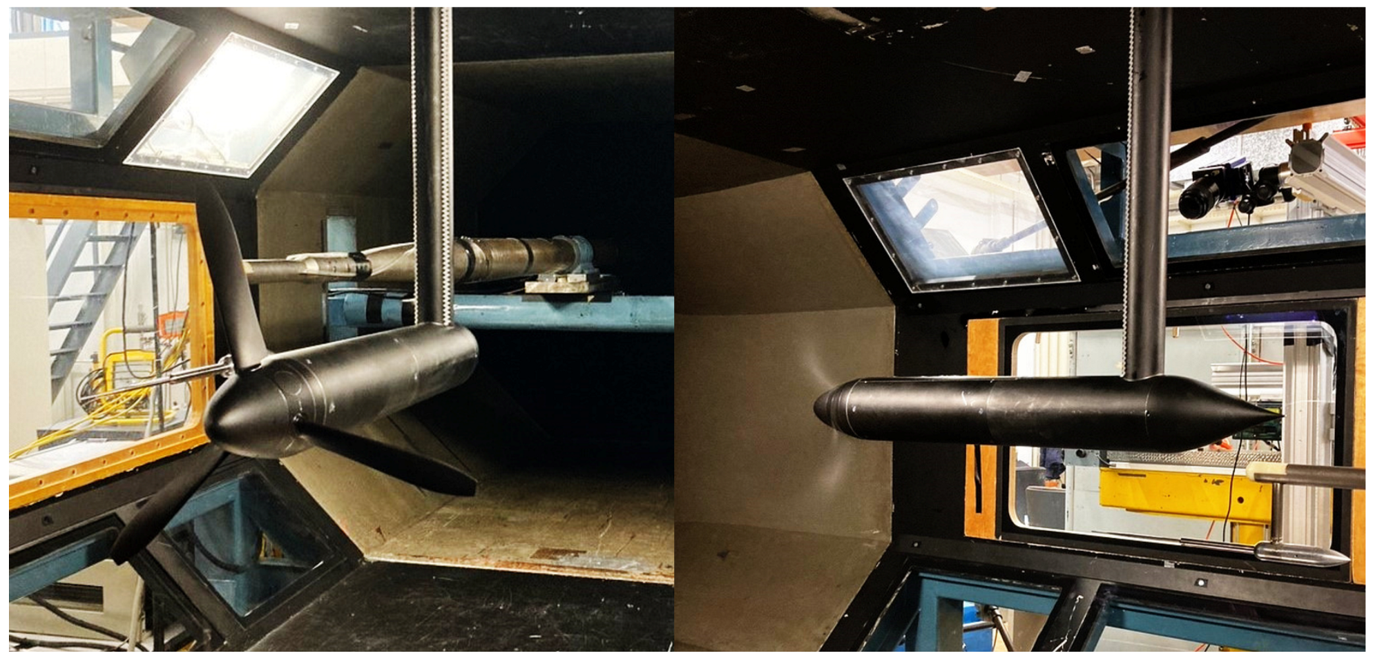
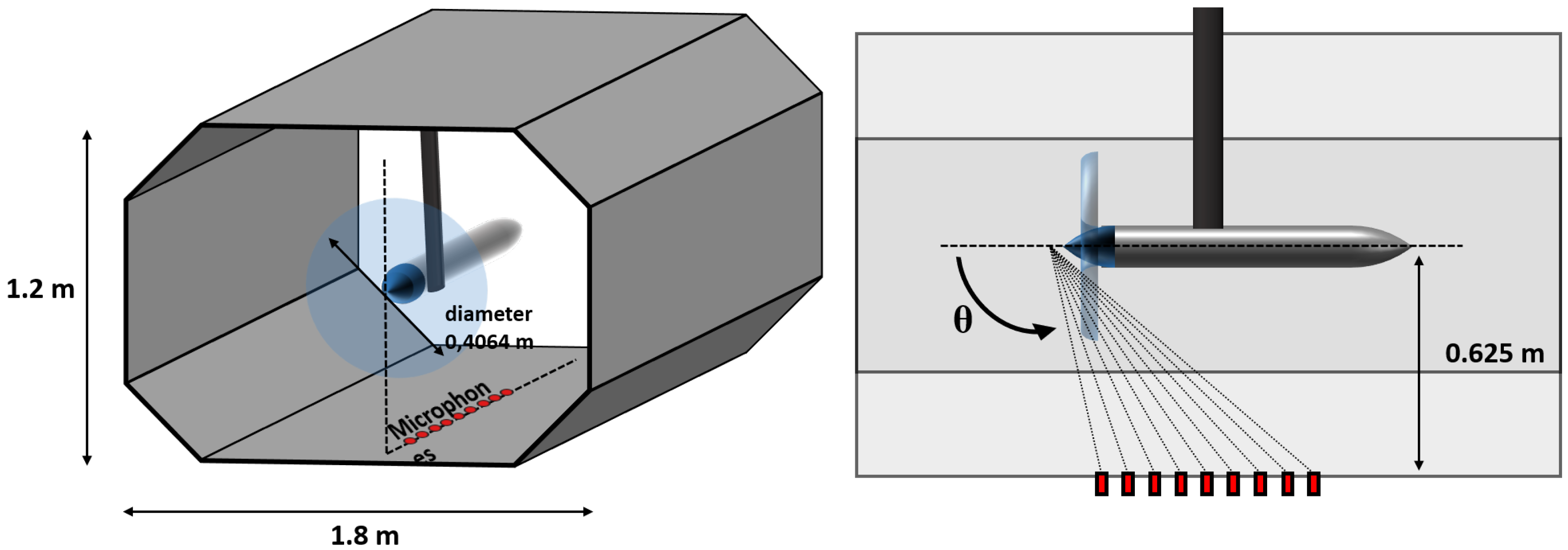
An isolated propeller experiment was performed in the low-speed Low-Turbulence Tunnel (LTT) at Delft University of Technology, as shown in Figure 2. The LTT features an octagonal closed test section of 1.80 m × 1.25 m and has a low inflow turbulence level of 0.02–0.03% at 40 m/s. For a schematic representation of the experimental setup within the wind tunnel, see Figure 3. The experiment was performed using a three-bladed propeller with a blade design representative of previous-generation turboprop aircraft. The propeller diameter was D = 0.4064 m. The propeller features modified ARA-D profiles, with a maximum thickness-to-chord ratio (t/c) of 0.05 at the tip, 0.12 at r/R = 0.5 and 0.20 at the hub. The distance between the propeller center and the wind tunnel wall was 0.625 m in the vertical direction and 0.9 m in the lateral direction.
The loads of the propeller were measured using a six-component internal load cell and an external balance, to enable separation of the interaction effects between propeller slipstream and support structure. A plate containing 9 microphones was placed in the floor of the test section to quantify the acoustic output of the propeller. For the microphone position, see Figure 3. In the linear microphone array, five LinearX M51-type and four LinearX M53-type microphones were used in line to the rotation axis. The microphones were characterized by maximum SPLs of 150 dB and 130 dB, respectively, a diameter of 1/2 inch and a frequency range between 20 Hz and 20 kHz. The microphones were properly calibrated by means of a piston phone GRAS 42AA, which outputs a tonal noise signal with amplitude 114 dB at a frequency of 250 Hz and an uncertainty lower than 0.09 dB for a confidence level of 99%.
A constant free stream velocity of 30 m/s was used and the rotational speed was varied to achieve both propulsive and energy harvesting conditions. For the acoustic measurements, all results discussed in this paper were obtained at a fixed blade pitch setting of 15 degrees at 70% of the radius. Pressure–time series were acquired for 30 s with a sampling frequency of 51.2 kHz. Note that the LTT is not an anechoic tunnel and hence acoustic reflections will have been present that will have affected the measurement results. For this reason, the pressure–time series were pre-processed using a low-pass filter to cancel out the frequency range below 100 Hz, which was dominated by noise from the wind-tunnel fan. For the purposes of this study, therefore, the results can be considered reliable as there are several orders of magnitude between these two noise sources.
In addition, for further confirmation of the validity of the results, the noise related to the wind tunnel was quantified and it was, on average, more than 20 dB lower than the noise produced by the propeller.
To determine the effective velocity in the closed test section, wind tunnel corrections are (normally) needed, but in the case presented here the combination of solid and slipstream blockage amounted to a blockage effect on a velocity of about −0.5% for the positive thrust case, +0.2% for the 0 thrust case and +1.5% for the regenerative case. This means that the corrected freestream velocity would be −0.5% up to +1.5% different for the different cases. For the purpose of the comparison in this paper, corrections are not considered required because the comparison between the different loading conditions will not change (without walls the same loading conditions would be obtained at a slightly different advance ratio).
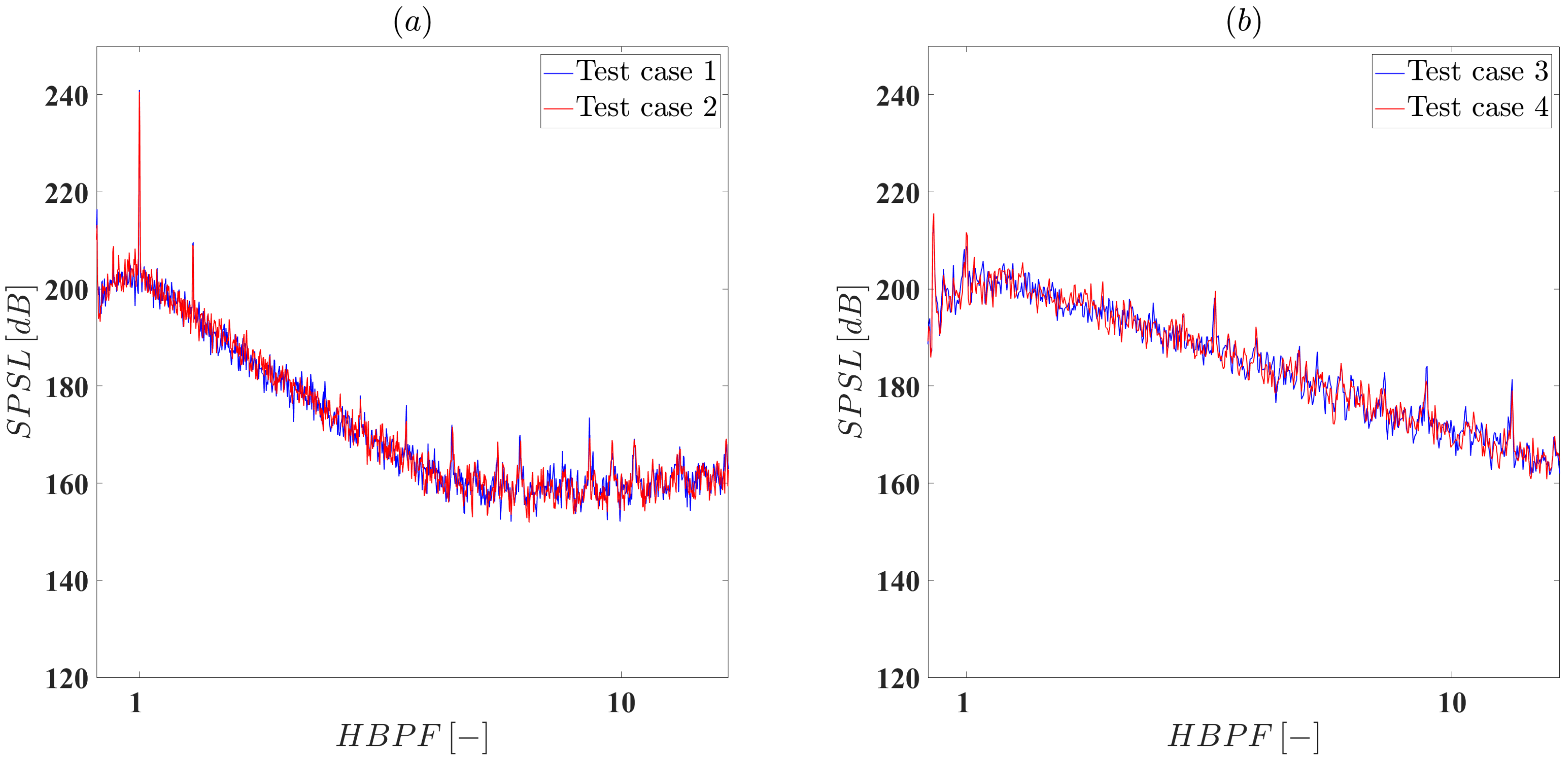
In addition, several tests at constant advance ratio J were performed in order to check the repeatability of the experiment. As an example, Figure 4 shows a noise spectrum for the propulsive and the energy harvesting configurations. This figure confirms the repeatability of the experimental measurements, thereby providing confidence in the quality of the data set. Moreover, in order to obtain a quantitative measure, the overall sound pressure level (OASPL) was calculated for all the repeated test cases and the difference between repeated measurements was in the order of 1%, whereas it is less than 3% when considering the band-limited OASPL relative to the first harmonic.
2.2. Proper Orthogonal Decomposition
In order to investigate the different sources of noise involved, a proper orthogonal decomposition (POD) analysis was performed; in particular, an innovative application of such investigation tool was defined.
POD is a common mathematical procedure for extracting a basis for modal decomposition from an ensemble of signals. The method has been widely used in turbulent flows since it provides a low-dimensional representation of a characteristic large-scale structure by decomposing it into a set of uncorrelated, data-dependent components. The components are the eigenfunctions of a two-point correlation tensor. For a comprehensive review about the mathematical formulation of proper orthogonal decomposition and its application to turbulent flows the reader may refer to the large body of literature (e.g., [30,31,32]).
In this paper, a novel application of POD is reported; the modal decomposition is applied to a pressure–time series in the near field in order to split the signal into its components: tonal and broadband. The starting point for the innovative formulation presented here is the so-called snapshot POD [31,33]. The idea is to apply windowing to the pressure–time series and, subsequently, to re-arrange the obtained vector in a matrix .
This will lead to calculation of the autocovariance matrix as:
Then, the procedure is to resolve the corresponding eigenvalue problem:
and to re-order the obtained solutions by the size of the obtained eigenvalues:
The eigenvectors of Equation (5) comprise the basis of the POD modes , defined as:
where is the n-th component of the eigenvectors corresponding to of Equation (5) and represents the discrete 2-norm defined as (where is a generic vector of N components).
The time signal can be reconstructed as:
where denotes the POD coefficients defined as the projection of the pressure signal onto the POD modes:
The matrix is composed of the POD modes as
Having imposed Equation (6) it is ensured that the most energetic mode is the first one. Generally, this means that the first mode is associated with the fundamental harmonics and thus the dominant tonal peak at the blade-passage frequency for propeller noise is reflected in the first POD mode. It is important to underline that for isolated propellers the main source of tonal noise is ascribable to the fundamental tone at the blade passage frequency, while the amplitudes of the higher harmonics are irrelevant and become smaller with increasing harmonic number. Therefore, the tonal noise component can be reconstructed correctly by looking at the first few modes.
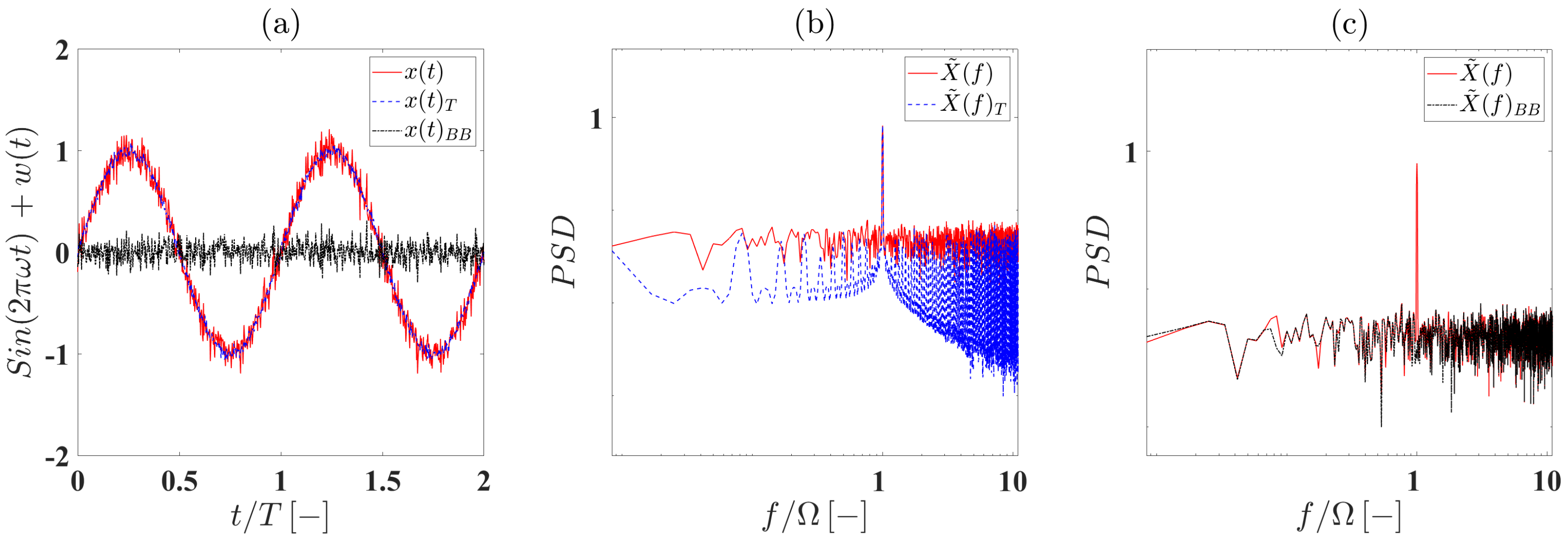
Figure 5 reports the application of this innovative separation technique to a synthetic signal: a sine wave with the addition of white noise. In more detail, Figure 5a reports the synthetic signals employed for the validation and the reconstructed components in time domain; Figure 5b shows the reconstructed tonal components compared with the original one in the frequency domain. Finally, Figure 5c reports the Fourier transform of the broadband components compared with the Fourier transform of the raw signal. These figures show very good agreement in both time, see Figure 5a, and frequency domains, Figure 5b,c, for the obtained reconstructed signals compared to the original one. The main evidence is that the reconstructed signals fit the original one perfectly in the time domain, as can be seen in Figure 5a. Moreover, in the frequency domain, it can be seen that the tonal peak of the sine wave is perfectly described (see the region ) by the decomposed signal, while in the other frequency regions the reconstructed tonal signal has less intensity than the original signal. Looking at the broadband counterpart instead it becomes clear that the tonal peak is not present anymore and the reconstructed signal fits perfectly the noisy part of the raw signal.
Such results can be interpreted as a validation of the presented strategy so it can represent a powerful tool with which to study a time series for the application where a periodic effect is embedded in a broadband phenomenon, like the one investigated in this manuscript.
2.3. Wavelet Transform
Wavelet transform analysis has become a common tool for the study of localized variations of power embedded in a time series. The wavelet transform (WT) permits expansion of a space/time history on a large variety of suitable functions. This feature makes the WT very interesting in a wide range of applications [34,35,36,37]. One of the main properties of the WT is its duality in both time and frequency domains, allowing determination of both the dominant modes of variability and how those modes vary in time. Consequently, the WT often better fits waves present in nature and with higher convergence velocity than the corresponding Fourier problem. The Fourier transform (FT) uses sine and cosine basis functions that have infinite span and are globally uniform in time. Consequently, the FT does not contain any time signal dependence and cannot provide any local information regarding the time evolution of its spectral characteristics [38]. However, WT uses generalized basis functions with a flexible resolution in frequency and time. As a result, by using the WT it is possible to achieve the optimal resolution with the lowest number of basis functions [38].
WT can be regarded as an evolution of the Fourier transform and the application fields are almost the same [39]. However, some fundamental differences can be found. Both the transformations are based on projection on an orthogonal basis function, and for this reason they both are invertible. Nevertheless, the FT basis is composed of sine and cosine functions; conversely, an infinite number of basis functions can be found for WT, as long as the admissibility criterion is satisfied [40,41]. These properties permit decomposition of a space/time series among a great variety of suitable functions, allowing selection of a basis specific for each problem [39].
In order to carry out a continuous wavelet transform (CWT), the first step is the choice of a proper wavelet function, called the mother wavelet . can be real or complex. In this study case, the mother wavelet used is the Morlet function, which is a complex solution of the wave equation [42], defined as:
where t is the dimensionless time and is the wavelet frequency center.
Starting from the mother wavelet , a family of continuously translated and dilated wavelets (the orthogonal basis functions) can be generated and normalized in the energy norm:
where s and are two real positive numbers called scaling parameter and time shifting, respectively. By varying s and , it is possible to represent the amplitude of any features versus the scale and how this amplitude varies with time in a single picture. In the present study, L-2 normalization has been applied to the mother wavelet thus and:
Finally, the CWT is defined as:
where is the wavelet coefficient and is the complex conjugate of the dilated and translated mother wavelet function.
One of the main differences between WT and Fourier transform is that, for a non-sinusoidal periodic signal, the latter spreads the energy content across several sub-harmonics. However, the former gives back only a few components with significant energy content.
In order to maintain a connection between these two transformations it is possible to convert the scaling factor s into a pseudo-frequency by using the following equation:
3. Results
The pressure fluctuations in the near-field were measured for different propeller operational conditions. The test matrix is composed of several measurements. The corresponding values of pitch angle , rotational velocity and advance ratio J are listed in Table 1. For brevity, the most interesting results are reported in this paper. These are concerned with the propeller operational conditions of maximum efficiency in the propulsive regime, the transitional regime (namely the crossing point between the propulsive and the regenerative configurations) and, finally, the most efficient regime in energy harvesting configuration at zero thrust. The blade pitch angle was fixed and the maximum efficiency values are to be considered exclusively as related to this specific configuration. These 3 case studies are related to 3 different rotational speeds, which are consequently characterized by different tip Mach numbers and different Reynolds numbers. As a result, the loading over the blade is very different in the 3 cases, leading to some variation in the propeller behavior.
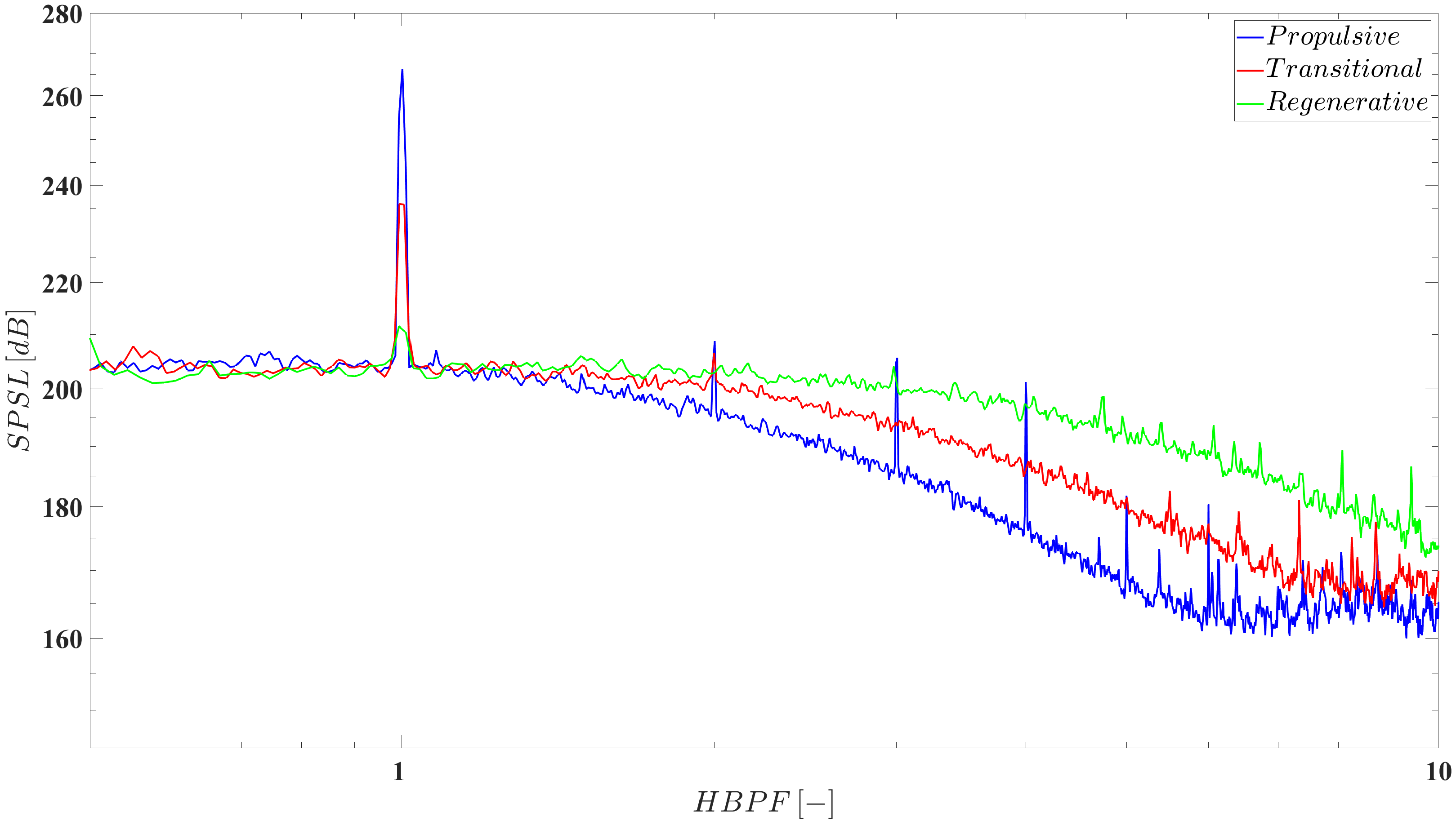
In order to evaluate the difference between the considered operational conditions, a spectral analysis was carried out. Figure 6 reports the noise spectra in a normalized form of the sound pressure spectrum level (SPSL) defined as:
where is the power spectral density of the pressure time history, is the frequency resolution and is the reference pressure equal to Pa (threshold of human hearing). In addition, the spectra are represented in nondimensional frequency; specifically, the harmonics of the blade passing frequency are reported, defined as:
where f is the frequency of sound emissions in Hz, B is the number of blades (for the present study ) and is the rotational velocity expressed in rad/s. The main observation is that when moving from the propulsive to the energy harvesting configuration, the most relevant noise source changes with a transfer of energy from the first harmonic () to the broadband counterpart at higher frequency. Such effect results in an increase in the noise amplitude in energy-harvesting mode for HBPF greater than 3 compared to the propulsive condition. In addition, the higher-order harmonics, observable for , are almost hidden in the broadband noise floor in both the transitional and regenerative conditions, while they appear evident in the propulsive regime. According to the literature [17,23,43,44], tonal noise can be associated with aerodynamic loading and its thickness over the blade. In the energy harvesting condition, the absolute loading on the blade was smaller than in the propulsive regime. This is because of the less efficient production of lift in this regime and is also due to the lower tip Mach number. This leads to a reduction in tonal noise. At the same time, in this configuration, the propeller is working in off-design condition and it generates more intense turbulent structures that result in increased broadband noise [16].
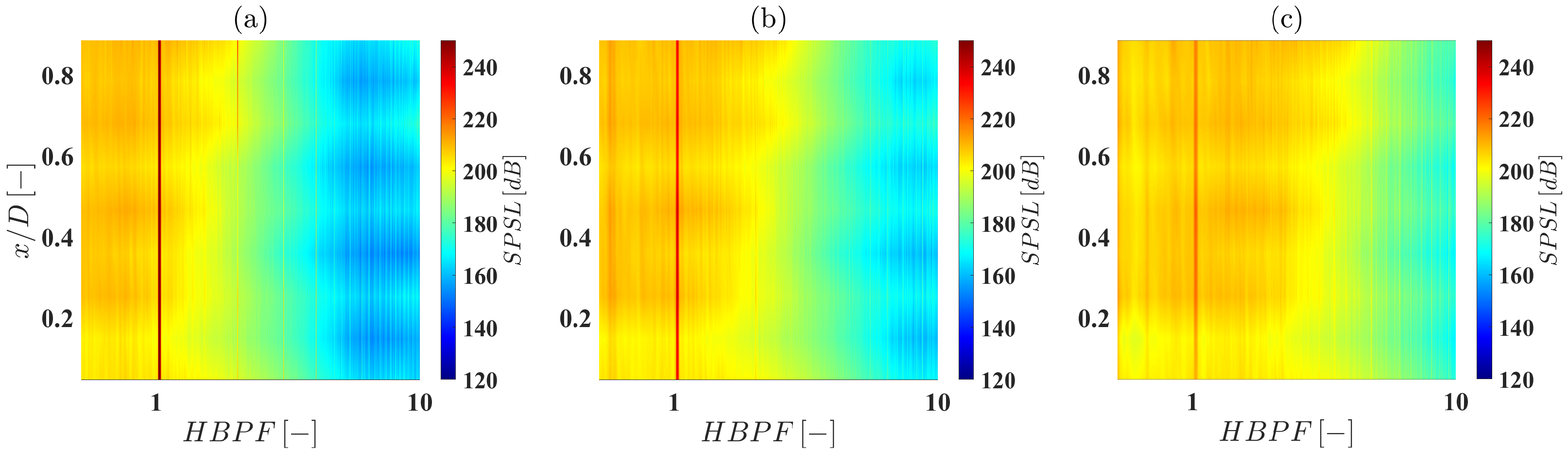
To further clarify these aspects, a space–frequency representation of the noise spectra is reported in Figure 7 in order to investigate the evolution in the axial direction with respect to the propeller center. Observing Figure 7c, it appears evident that the broadband region is much more developed and the first harmonic is strongly damped for the energy harvesting configuration compared to the propulsive mode. However, for the propulsive condition (Figure 7a), most of the energy is associated with the first harmonic. Moreover, the transitional configuration presents a strong peak at (see both Figure 6 and Figure 7), but the higher-order harmonics have been eliminated, resulting in a small increase of the broadband noise in the high-frequency region. In this sense, the transitional configuration lies in between the other 2 operational conditions. In addition, for all 3 test cases, it is possible to observe an increase in the broadband component in the x-direction that is attributable to the dissipation of the vortices shedding from the propeller moving away from it.
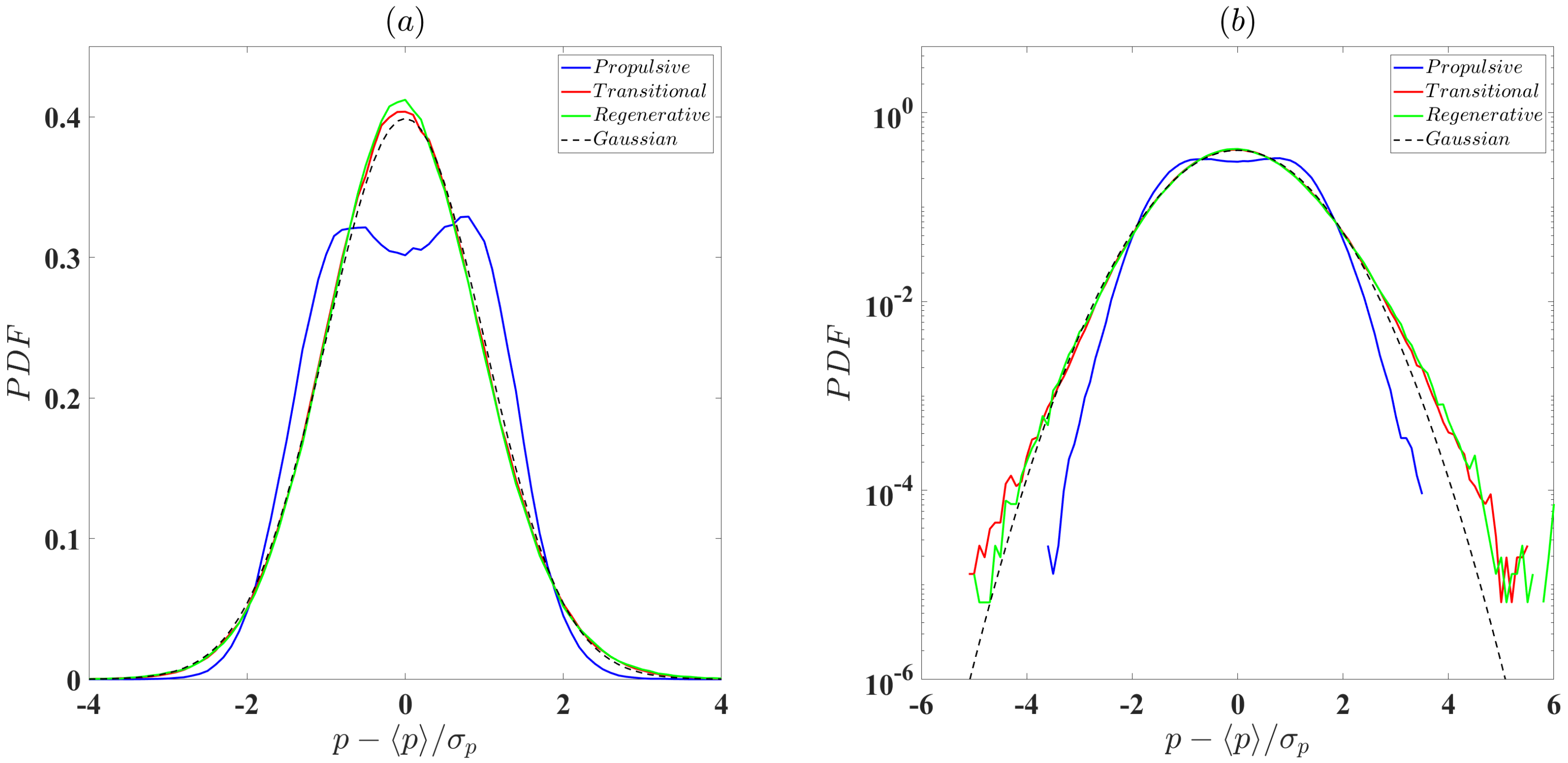
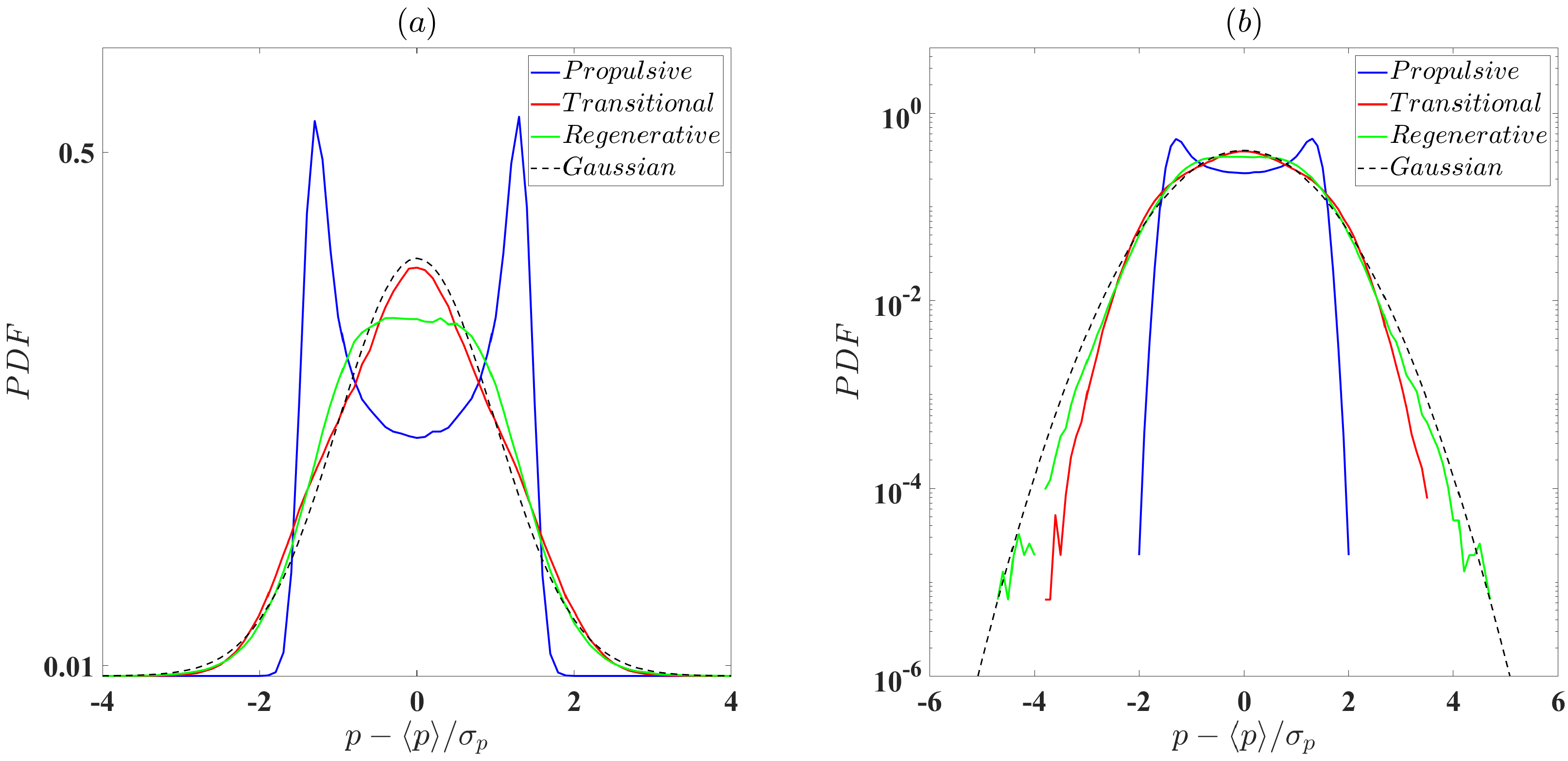
The effect of the operational regime on coherent structures embedded in the pressure time series can be demonstrated by analysis of the probability density function (PDF) of the pressure time history, as reported in Figure 8. The random variable is represented in reduced form in order to have zero mean and unit standard deviation. In addition, a Gaussian distribution was added in Figure 8 in order to make a comparison. The main difference between the distributions for the three operational conditions is that the propulsive condition displays in a bi-modal distribution characterized by a positive skewness, while the transitional and the regenerative configurations are described by a Gaussian distribution (see Figure 8a). Such effect can be interpreted as a loss in signal periodicity when the propeller is employed to harvest energy instead of generating thrust. Moreover, the distribution functions are also reported in logarithmic scale (Figure 8b); this alternative representation shows a departure of the tails of the distribution from the normal distribution for the transitional and regenerative regimes. Physically, this can be ascribed to the presence of coherent structures in the pressure time series, induced by the non-optimal operational conditions for the propeller. In these configurations, the propeller is generating a more turbulent flow structure resulting in higher broadband noise.
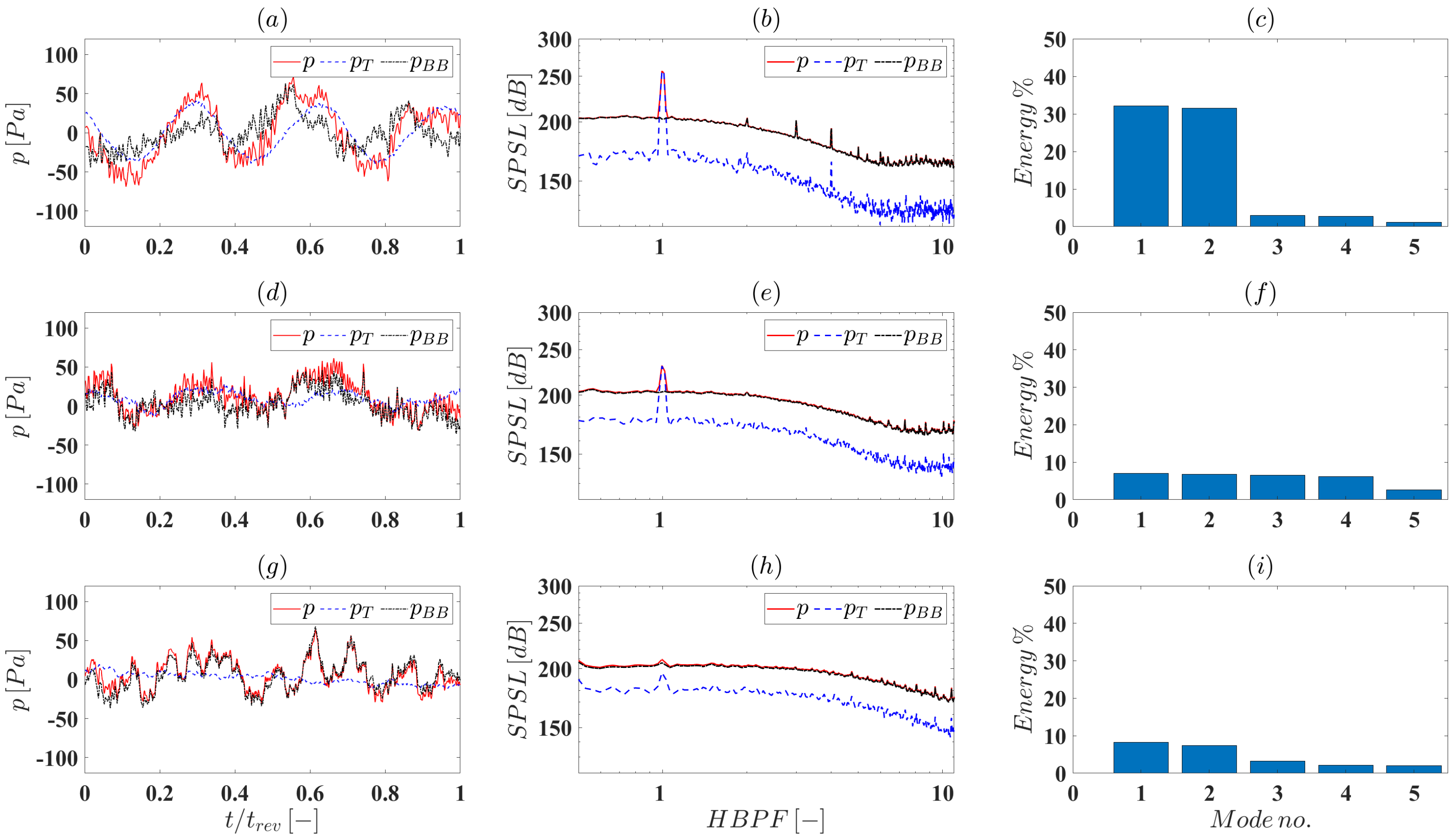
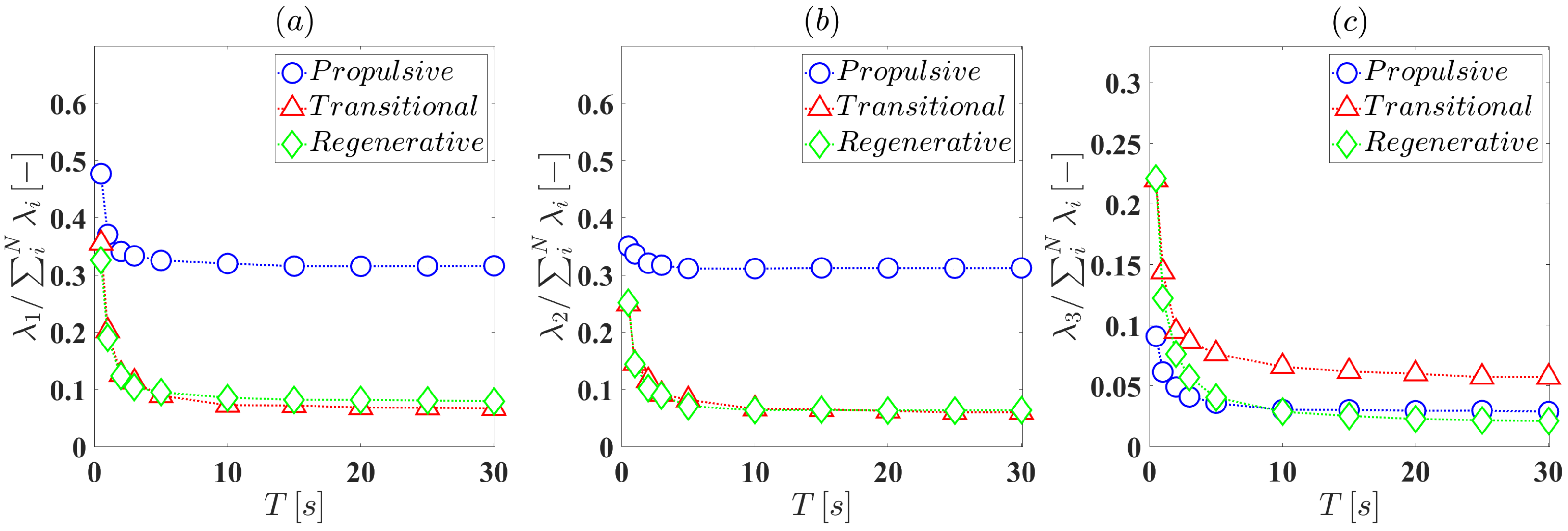
The observation of this dual nature of the signals suggests that decomposition of the noise components would enable a more detailed characterization of the individual noise sources involved. For this purpose, the POD-based signal decomposition, as defined in Section 2.2, has been applied and the results are reported in Figure 9. Before the results are discussed, it should be noted that a convergence study was first performed to assess whether the measurement duration was sufficiently long. Figure 10 shows the values taken by the eigenvalues, normalized with respect to the sum of all the eigenvalues, for different time intervals. It can be seen that after 10 s, the values obtained remain constant. This confirms that convergence has been achieved and thus ensures the reliability of the obtained results. In this figure, the first row (Figure 9a–c) shows the results for the propulsive configuration, the second row (Figure 9d–f) for the transitional configuration and the third row (Figure 9g–i) for the energy harvesting configuration. In the first column of Figure 9a,d,g, the time history of the raw signal is reported and, in order to enable comparison, the tonal and broadband counterparts are reported for each test case.
The time coordinate has been normalized by the revolution time in order to display one complete revolution of the propeller. Furthermore, the Fourier transform is addressed in the second column, see Figure 9b,e,h. Finally, the third column (Figure 9c,f,i) shows the percentage of energy associated with each POD mode, calculated as the ratio of the single eigenvalue to the sum of all eigenvalues. It is important to remember that the eigenvalues have previously been rearranged in descending order so that the first is associated with the most energetic mode that is to be considered ‘dominant’ (see Section 2.2). The pressure time series can be interpreted as the sum of the tonal and broadband components obtained by the decomposition. This aspect is fundamental in the fact that the tonal (or the broadband) component can even overcome the raw signal. The analysis in both time and frequency domains demonstrates the quality of the separation strategy, which describes the original signal with very good agreement. In addition, the presented algorithm does not involve a time delay between the raw and the reconstructed signals as it is typical for the filters already present in the literature. Looking at the bar diagram (Figure 9c,f,i), it appears evident that in the propulsive regime, where most of the energy of the pressure time signal is related to tonal noise, the first and second POD-modes contain more than 30% (38% and 36%, respectively) of the energy. This suggests that these modes are representative of the tonal noise while the higher-order modes can be ascribed to the broadband counterpart, which is characterized by lower energy. In fact, having recognized the tonal component of the pressure fluctuation fields in the POD modes of first and second order, it is ensured that our strategy, based on the projection on the low-order modes, is consistent and the results are in agreement with sound spectra and the PDFs seen previously in Figure 6, Figure 7 and Figure 8. The regenerative configuration, i.e., Figure 9g,h, shows unexpected behavior. In the time history of the tonal component, a periodic component does not seem to be recognizable. Nevertheless, a tonal peak can be observed in the frequency domain, but it is associated with much less energy than the broadband component. Moreover, Figure 9i shows that the energy is distributed among several POD modes, whereas in the propulsive regime it is almost totally associated with the first and second modes.
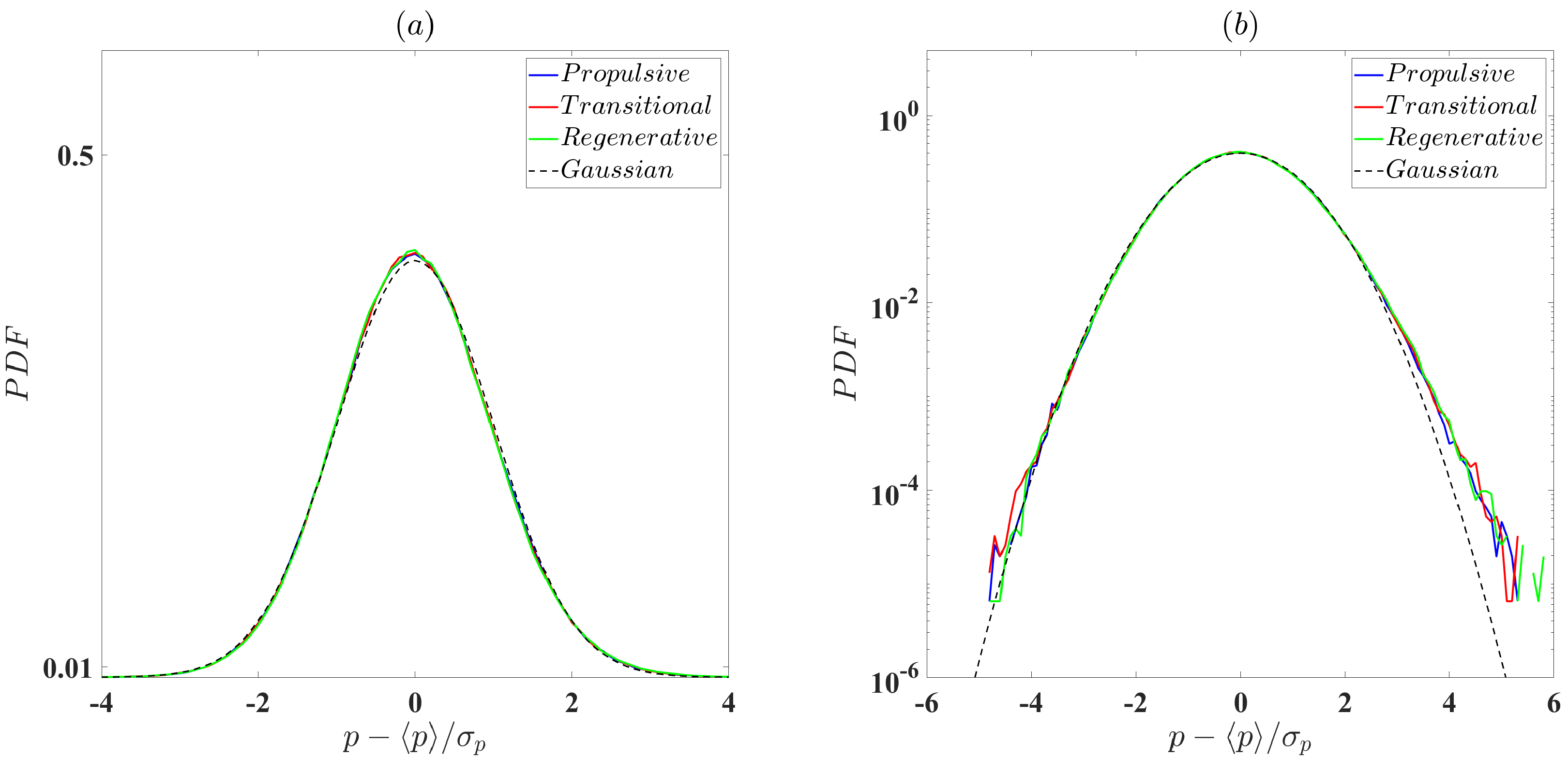
Having defined such a powerful tool for decomposition allows accurate isolation of noise sources. For this purpose, the PDFs of the normalized pressure signal have been provided for the tonal and broadbrand parts of the pressure time series. Figure 11 reports the results regarding the tonal components in both linear and logarithmic scales. Thereby, results regarding the broadband noise components are shown in Figure 12. The results are in agreement with those obtained from the raw pressure time series (see Figure 8), where the propulsive regime displays a bi-modal distribution. However, the transitional condition presents a normal distribution. It is interesting to note that the regenerative condition presents a departure from the Gaussian distribution since the distribution function tends to a bi-modal one, confirming the tonal component observed in Figure 9. A bi-modal distribution is ascribable to a periodic phenomenon. Conversely, a random phenomenon is expressed in a Gaussian PDF. Therefore, the results obtained confirm what has been seen previously; that is, only in the propulsive case is a tonal component observable, while in the transitional and regenerative cases the tonal component is embedded within the broadband component, which dominates the acoustic emissions at the operational conditions considered in this paper.
Moreover, Figure 12 reports the probability distribution functions for the broadband component. In this case, all the operational conditions are characterized by a normal distribution as expected. Nevertheless, the logarithmic scale (Figure 12b) highlights a positive skewness of the distributions and also a departure from the Gaussian distribution regarding the tails of the distributions, confirming the presence of coherent structures embedded in the time series. The distribution functions suggests that the increase in the broadband noise may be ascribed to the off-design operational condition of the propeller, which results in more vortex shedding at the trailing edge. Such effect can induce a more turbulent wake region. In addition, the decomposition technique herein proposed may be a useful tool for isolating the intermittent structure embedded in a time series; this aspect needs further investigation.
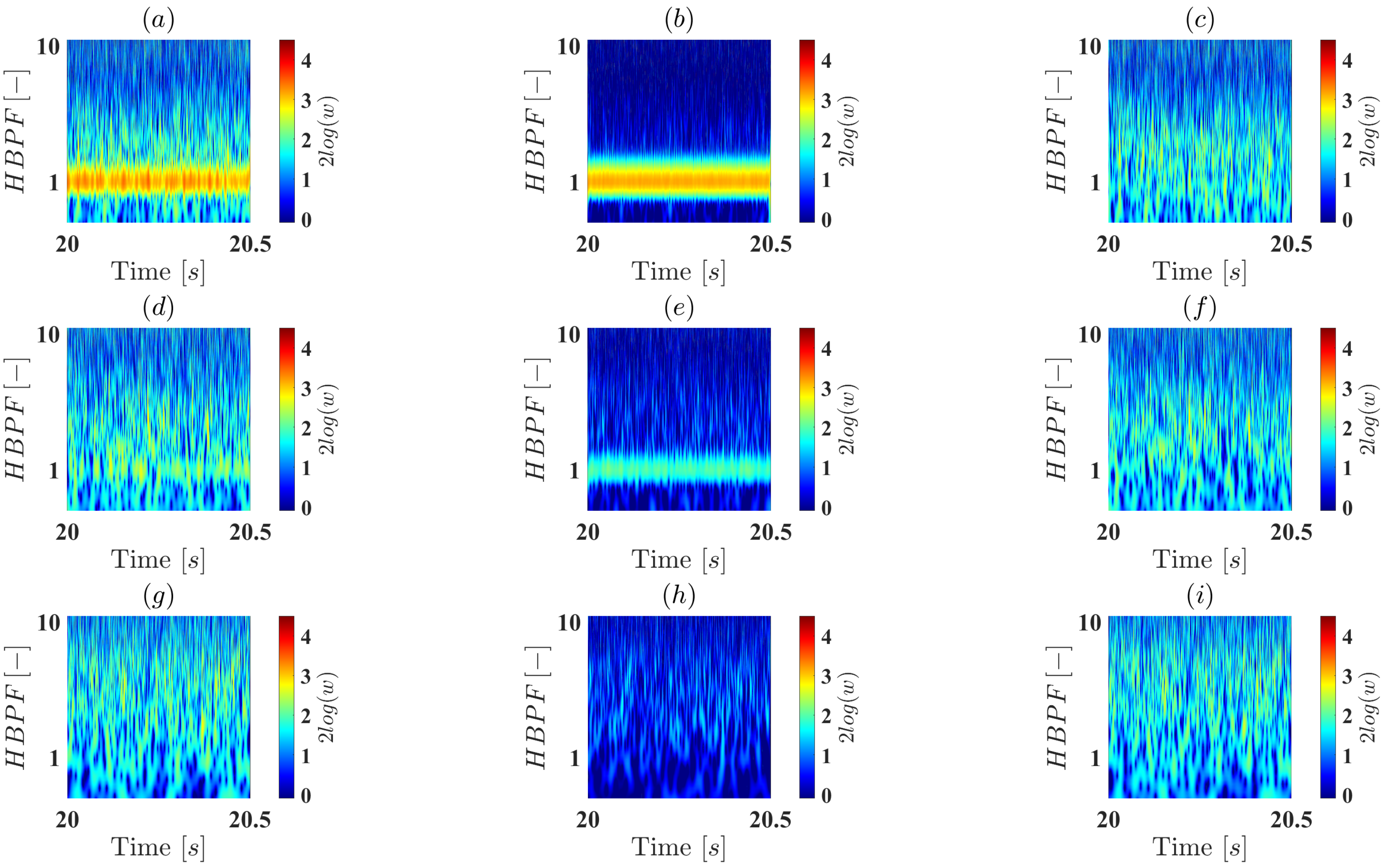
Finally, a time–frequency representation of the decomposed signals is reported in Figure 13 in terms of wavelet intensity. The first column (Figure 13a,d,g) reports the wavelet transform for the original pressure signals for each study case, the second column (Figure 13b,e,h) shows the obtained tonal parts and the third column (Figure 13c,f,i) represents the broadband component of the time series. The wavelet transform with its dual definition in both time and frequency domains is a very useful tool in the analysis of turbulent fields. Furthermore, by using WT and POD decomposition it is possible to achieve a better understanding of the occurring phenomena. Figure 13f,i reveal the presence of some intermittent events of low time scales that are related to the raising of the distribution tails. The increase in the broadband noise for the regenerative configuration in respect to the propulsive one, observed in Figure 6 and Figure 7, can be ascribed to these events. Conversely, for the propulsive regime, most of the energy can be ascribed to the tonal noise component, resulting in a strong peak at over the entire time domain. To conclude, it can be assumed that if the propeller is working to recover energy, consequently the load on the blade tends to cancel, and the tonal component is eliminated. Moreover, since it is working in an off-design condition, intermittent flow structures are generated that cause a strong increase in the broadband component in the high-frequency region.
In Figure 9h, a tonal peak can be observed that is not present in Figure 13g, even though these figures represent the same test case. Such result can be ascribed to a fluctuating tonal component embedded in the broadband signal, which is captured by the Fourier transform, because it averages the signal, but the WT does not recognize it in the investigated time window. The WT, because of its dual nature, helps us to understand the presence of the tonal peak of Figure 9h; when looking just at the FT it may seem as if there is an error in the algorithm. However, it can be interpreted as a mathematical artifact related to the procedure employed in the FT method. In this sense, the WT gives us a further validation of the decomposition strategy in addition to the physical consideration previously reported.
4. Conclusions
The noise signature related to the usage of a propeller to recover energy has been investigated by means of microphone measurements.
The spectral analysis demonstrates that when the propeller is employed as a wind-turbine the broadband noise emissions increase. Conversely, in the propulsive regime the most of the energy is associated with the tonal noise component. In the energy harvesting condition, the propeller is working off-design since the load on the blade is very low resulting in a reduction in the tonal noise.
The statistical analysis clarifies this aspect: the probability distribution function in energy harvesting configuration shows a departure from the Gaussian distribution, revealing the presence of coherent structures embedded in the pressure–time series. Since the propeller is used in order to harvest energy, it is working in off-design conditions resulting in an increase in separation along the blade.
Moreover, a novel separation technique based on proper orthogonal decomposition was presented that allows decomposition of the noise components into tonal and broadband contributions. The results in both time and frequency domains confirm the initial conclusion and also prove the quality of the decomposition strategy employed. The probability density functions for the tonal and broadband components individually demonstrate the considerations already drawn. The tonal component of the propulsive configuration is characterized by a bi-modal distribution typical of a sinusoidal periodic phenomenon, while the transitional and energy harvesting configurations present a normal distribution confirming that the broadband contribution is the most relevant for these two configurations. In addition, the analysis of the broadband components clarifies the presence of intermittent events within the pressure–time series. Such results suggest the need for further investigation; consequently a wavelet-based analysis was provided. The wavelet intensity in the time–frequency domain confirms the presence of vortex structures in the pressure field, to which the increase in broadband noise can be ascribed.
In conclusion, in order to achieve eco-friendly propulsion of an aircraft, it is possible to employ the propellers to recover energy in some particular flight stages. Such solution influences the aircraft noise emissions, suggesting the need for a combination of noise control strategies. In this way it is possible to reduce the noise emissions in all the flight conditions that the mission involves.
Author Contributions
Formal analysis and writing, P.C., E.M., R.N., T.S. and T.P.; Software P.C., E.M. and T.P.; Investigation R.N. and T.S. All authors have read and agreed to the published version of the manuscript.
Funding
This project received funding from the European Union’s Horizon 2020 Research and Innovation programme under Grant Agreement No. 875551.
Institutional Review Board Statement
Not applicable.
Informed Consent Statement
Not applicable.
Data Availability Statement
Not applicabe.
Acknowledgments
The research leading to these results was performed in the frame of the FUTPRINT50 Project. This project received funding from the European Union’s Horizon 2020 research and innovation programme under grant agreement No. 875551.
Conflicts of Interest
The authors declare no conflict of interest.
Abbreviations
The following abbreviations are used in this manuscript:
| DEP | Distributed electric propulsion |
| EP | Electric propulsion |
| FT | Fourier transform |
| HBPF | Harmonics of the blade passing frequency |
| HEP | Hybrid-electric propulsion |
| POD | Proper orthogonal decomposition |
| SPSL | Sound pressure spectrum level |
| WT | Wavelet transform |
References
- Follen, G.; Del Rosario, R.; Wahls, R.; Madavan, N. NASA’s Fundamental Aeronautics Subsonic Fixed Wing Project: Generation N+3 Technology Portfolio; Technical Report; Society of Automotive Engineers (SAE): Los Angeles, CA, USA, 2007. [Google Scholar]
- Guynn, M.D.; Berton, J.; Tong, M.; Haller, W. Advanced single-aisle transport propulsion design options revisited. In Proceedings of the 2013 Aviation Technology, Integration, and Operations Conference, Los Angeles, CA, USA, 12–14 August 2013; p. 4330. [Google Scholar]
- International Civil Aviation Organization. Technology Standards; ICA: Wayne, PA, USA, 2011. [Google Scholar]
- Brelje, B.J.; Martins, J.R. Electric, hybrid, and turboelectric fixed-wing aircraft: A review of concepts, models, and design approaches. Prog. Aerosp. Sci. 2019, 104, 1–19. [Google Scholar] [CrossRef]
- De Vries, R.; Brown, M.; Vos, R. Preliminary sizing method for hybrid-electric distributed-propulsion aircraft. J. Aircr. 2019, 56, 2172–2188. [Google Scholar] [CrossRef]
- Friedrich, C.; Robertson, P. Hybrid-electric propulsion for aircraft. J. Aircr. 2015, 52, 176–189. [Google Scholar] [CrossRef]
- Gunnarsson, G.; Skúlason, J.B.; Sigurbjarnarson, Á.; Enge, S. Regenerative Electric/hybrid Drive Train for Ships RENSEA II; Nordic Innovation Publication: Oslo, Norway, 2016; Available online: http://urn.kb.se/resolve?urn=urn:nbn:se:norden:org:diva-5503 (accessed on 21 June 2022).
- Barnes, J. Flight without Fuel–Regenerative Soaring Feasibility Study; Technical Report, SAE Technical Paper; SAE: Warrendale, PA, USA, 2006. [Google Scholar]
- Barnes, J. Regenerative electric flight synergy and integration of dual role machines. In Proceedings of the 53rd AIAA Aerospace Sciences Meeting, Kissimmee, FL, USA, 5–9 January 2015; p. 1302. [Google Scholar]
- Galvao, F. A Note on Glider Electric Propulsion. Tech. Soar. 2012, 36, 94–101. [Google Scholar]
- MacCready, P. Regenerative battery-augmented soaring. Tech. Soar. 1999, 23, 28–32. [Google Scholar]
- Binder, N.; Courty-Audren, S.; Duplaa, S.; Dufour, G.; Carbonneau, X. Theoretical analysis of the aerodynamics of low-speed fans in free and load-controlled windmilling operation. J. Turbomach. 2015, 137, 101001. [Google Scholar] [CrossRef]
- Ortolan, A.; Courty-Audren, S.; Binder, N.; Carbonneau, X.; Rosa, N.; Challas, F. Experimental and numerical flow analysis of low-speed fans at highly loaded windmilling conditions. J. Turbomach. 2017, 139, 071009. [Google Scholar] [CrossRef]
- Cherubini, A.; Papini, A.; Vertechy, R.; Fontana, M. Airborne Wind Energy Systems: A review of the technologies. Renew. Sustain. Energy Rev. 2015, 51, 1461–1476. [Google Scholar] [CrossRef] [Green Version]
- Erzen, D.; Andrejasic, M.; Kosel, T. An Optimal Propeller Design for In-Flight Power Recuperation on an Electric Aircraft. In Proceedings of the 2018 Aviation Technology, Integration, and Operations Conference, Atlanta, GA, USA, 25–29 June 2018; p. 3206. [Google Scholar]
- Goyal, J.; Sinnige, T.; Avallone, F.; Ferreira, C. Aerodynamic and Aeroacoustic Characteristics of an Isolated Propeller at Positive and Negative Thrust. In Proceedings of the AIAA Aviation 2021 Forum, Virtual Event, 2–6 August 2021; p. 2187. [Google Scholar]
- Gur, O.; Rosen, A. Design of a Quiet Propeller for an Electric Mini. J. Propul. Power 2009, 25, 717–728. [Google Scholar] [CrossRef]
- Farassat, F.; Succi, G. A review of propeller discrete frequency noise prediction technology with emphasis on two current methods for time domain calculations. Top. Catal. 1980, 71, 399–419. [Google Scholar] [CrossRef]
- Farassat, F. Linear acoustic formulas for calculation of rotating blade noise. AIAA J. 1981, 19, 1122–1130. [Google Scholar] [CrossRef]
- Farassat, F.; Brentner, K.S. The acoustic analogy and the prediction of the noise of rotating blades. Theor. Comput. Fluid Dyn. 1998, 10, 155–170. [Google Scholar] [CrossRef]
- Succi, G.; Munro, D.; Zimmer, J. Experimental Verification of Propeller Noise Prediction. AIAA J. 1982, 20, 1483–1491. [Google Scholar] [CrossRef]
- Pagano, A.; Barbarino, M.; Casalino, D.; Federico, L. Tonal and broadband noise calculations for aeroacoustic optimization of a pusher propeller. J. Aircraft 2010, 47, 835–848. [Google Scholar] [CrossRef]
- Sinibaldi, G.; Marino, L. Experimental analysis on the noise of propellers for small UAV. Appl. Acoust. 2013, 74, 79–88. [Google Scholar] [CrossRef]
- Intravartolo, N.; Sorrells, T.; Ashkharian, N.; Kim, R. Attenuation of Vortex Noise Generated by UAV Propellers at Low Reynolds Numbers. In Proceedings of the 55th AIAA Aerospace Sciences Meeting, Grapevine, TX, USA, 9–13 January 2017. [Google Scholar] [CrossRef]
- Pagliaroli, T.; Candeloro, P.; Camussi, R.; Giannini, O.; Panciroli, R.; Bella, G. Aeroacoustic Study of small scale Rotors for mini Drone Propulsion: Serrated Trailing Edge Effect. In Proceedings of the 2018 AIAA/CEAS Aeroacoustics Conference, Atlanta, GA, USA, 25–29 June 2018. [Google Scholar] [CrossRef]
- Zawodny, N.S.; Boyd, D.D., Jr.; Burley, C.L. Acoustic Characterization and Prediction of Representative, Small-Scale Rotary-Wing Unmanned Aircraft System Components. In Proceedings of the 72nd American Helicopter Society (AHS) Annual Forum, West Palm Beach, FL, USA, 17–19 May 2016. [Google Scholar]
- Truong, A.; Papamoschou, D. Harmonic and broadband separation of noise from a small ducted fan. In Proceedings of the 21st AIAA/CEAS Aeroacoustics Conference, Dallas, TX, USA, 22–26 June 2015; p. 3282. [Google Scholar]
- Sree, D. A novel signal processing technique for separating tonal and broadband noise components from counter-rotating open-rotor acoustic data. Int. J. Aeroacoust. 2013, 12, 169–188. [Google Scholar] [CrossRef]
- Sree, D.; Stephens, D. Tone and broadband noise separation from acoustic data of a scale-model counter-rotating open rotor. In Proceedings of the AIAA/CEAS Aeroacoustics Conference, Atlanta, GA, USA, 16–20 June 2014; pp. 2014–2744. [Google Scholar]
- Berkooz, G.; Holmes, P.; Lumley, J. The proper orthogonal decomposition in the analysis of turbulent flows. Annu. Rev. Fluid Mech. 1993, 25, 539–575. [Google Scholar] [CrossRef]
- Sirovich, L. Turbulence and the dynamics of coherent structures. III. Dynamics and scaling. Q. Appl. Math. 1987, 45, 583–590. [Google Scholar] [CrossRef] [Green Version]
- Kirby, M.; Boris, J.; Sirovich, L. A proper orthogonal decomposition of a simulated supersonic shear layer. Int. J. Numer. Methods Fluids 1990, 10, 411–428. [Google Scholar] [CrossRef]
- Meyer, K.; Pedersen, J.; Özcan, O. A turbulent jet in crossflow analysed with proper orthogonal decomposition. J. Fluid Mech. 2007, 583, 199–227. [Google Scholar] [CrossRef] [Green Version]
- Pagliaroli, T.; Mancinelli, M.; Troiani, G.; Iemma, U.; Camussi, R. Fourier and wavelet analyses of intermittent and resonant pressure components in a slot burner. J. Sound Vib. 2018, 413, 205–224. [Google Scholar] [CrossRef]
- Pagliaroli, T.; Pagliaro, A.; Patané, F.; Tatí, A.; Peng, L. Wavelet analysis ultra-thin metasurface for hypersonic flow control. Appl. Acoust. 2020, 157, 107032. [Google Scholar] [CrossRef]
- Pagliaroli, T.; Troiani, G. Wavelet and recurrence analysis for lean blowout detection: An application to a trapped vortex combustor in thermoacoustic instability. Phys. Rev. Fluids 2020, 5, 073201. [Google Scholar] [CrossRef]
- Mancinelli, M.; Pagliaroli, T.; Camussi, R.; Castelain, T. On the hydrodynamic and acoustic nature of pressure proper orthogonal decomposition modes in the near field of a compressible jet. J. Fluid Mech. 2018, 836, 998–1008. [Google Scholar] [CrossRef] [Green Version]
- Lau, K.M.; Weng, H. Climate signal detection using wavelet transform: How to make a time series sing. Bull. Am. Math. Soc. 1995, 76, 2391–2402. [Google Scholar] [CrossRef] [Green Version]
- Ashmead, J. Morlet Wavelets in Quantum Mechanics. Quanta 2012, 1, 58–70. [Google Scholar] [CrossRef] [Green Version]
- Farge, M. Wavelet transforms and their applications to turbulence. Annu. Rev. Fluid Mech. 1992, 24, 395–458. [Google Scholar] [CrossRef]
- Torrence, C.; Compo, G. A practical guide to wavelet analysis. Bull. Amer. Meteor. Soc. 1998, 79, 61–78. [Google Scholar] [CrossRef] [Green Version]
- Visser, M. Physical wavelets: Lorentz covariant, singularity-free, finite energy, zero action, localized solutions to the wave equation. Phys. Lett. A 2003, 315, 219–224. [Google Scholar] [CrossRef] [Green Version]
- Kurtz, D.; Marte, J. A Review of Aerodynamic Noise from Propellers, Rotors, and Lift Fans; Jet Propulsion Laboratory, California Institute of Technology: Passadena, CA, USA, 1970. [Google Scholar]
- Candeloro, P.; Nargi, R.; Patanè, F.; Pagliaroli, T. Experimental Analysis of Small-Scale Rotors with Serrated Trailing Edge for Quiet Drone Propulsion. In Journal of Physics: Conference Series; IOP Publishing: Bristol, UK, 2020; Volume 1589, p. 012007. [Google Scholar] [CrossRef]
Figure 1.
Schematic representation of the main broadband noise sources around an airfoil.

Figure 2.
Photos of the experimental setup employed for the measurement campaign at Delft University of Technology’s Low-Turbulence Tunnel.
Figure 2.
Photos of the experimental setup employed for the measurement campaign at Delft University of Technology’s Low-Turbulence Tunnel.

Figure 3.
Schematic representation of the experimental setup located within the wind tunnel.

Figure 4.
Repeatability test: comparison between noise spectra. (a) test performed at advance ratio J = 0.7. (b) test performed at advance ratio J = 1.2.
Figure 4.
Repeatability test: comparison between noise spectra. (a) test performed at advance ratio J = 0.7. (b) test performed at advance ratio J = 1.2.

Figure 5.
Application of the POD–based decomposition strategy to a synthetic signal: a noisy sine wave. (a) Signals, total and reconstructed, in the time domain; (b) the total and reconstructed tonal signals in the frequency domain; (c) the total and reconstructed broadband signals in the frequency domain.

Figure 6.
Dimensionless spectra of the near-field pressure signals for each operational condition.

Figure 7.
Contour map of the sound pressure spectrum level of the near-field pressure signals along the axial distance for each operational condition. (a) Propulsive configuration. (b) Transitional configuration. (c) Regenerative condition.
Figure 7.
Contour map of the sound pressure spectrum level of the near-field pressure signals along the axial distance for each operational condition. (a) Propulsive configuration. (b) Transitional configuration. (c) Regenerative condition.

Figure 8.
Probability density function of the near field pressure signals for each operational condition. The PDFs are reported in both linear (a) and logarithmic scales (b).
Figure 8.
Probability density function of the near field pressure signals for each operational condition. The PDFs are reported in both linear (a) and logarithmic scales (b).

Figure 9.
Application of the POD–based decomposition strategy to the test cases under analysis. (a) Time history of the raw pressure signal and of its tonal and broadband components for the propulsive regime. (b) Nondimensional spectra for the propulsive regime. (c) Energy percentage associated with the POD modes for the propulsive regime. (d) Time history of the raw pressure signal and of its tonal and broadband components for the transition regime. (e) Nondimensional spectra for the transitional regime. (f) Energy percentage associated with the POD modes for the transitional regime. (g) Time history of the raw pressure signal and of its tonal and broadband components for the regenerative configuration. (h) Nondimensional spectra for the regenerative configuration. (i) Energy percentage associated with the POD modes for the regenerative regime.

Figure 10.
Convergence analysis of the eigenvalues for the POD decomposition for each operational condition. (a) First eigenvalue ; (b) second eigenvalue ; (c) third eigenvalue .
Figure 10.
Convergence analysis of the eigenvalues for the POD decomposition for each operational condition. (a) First eigenvalue ; (b) second eigenvalue ; (c) third eigenvalue .

Figure 11.
Probability density function of the tonal component of pressure signals for each operational condition. The PDFs are reported in both linear (a) and logarithmic scales (b).
Figure 11.
Probability density function of the tonal component of pressure signals for each operational condition. The PDFs are reported in both linear (a) and logarithmic scales (b).

Figure 12.
Probability density function of the broadband component of pressure signals for each operational condition. The PDFs are reported in both linear (a) and logarithmic scales (b).
Figure 12.
Probability density function of the broadband component of pressure signals for each operational condition. The PDFs are reported in both linear (a) and logarithmic scales (b).

Figure 13.
Wavelet intensity of the near-field pressure signal for the raw signal and the tonal and broadband components for each operational condition. (a) for the propulsive regime. (b) for the propulsive regime. (c) for the propulsive regime. (d) for the transitional regime. (e) for the transitional regime. (f) for the transitional regime. (g) for the regenerative condition. (h) for the regenerative condition. (i) for the regenerative condition.


Table 1.
Pitch angle , rotational speed n and advance ratio J values for each operational condition investigated.
Table 1.
Pitch angle , rotational speed n and advance ratio J values for each operational condition investigated.
| Test Case | |||
|---|---|---|---|
| Propulsive | |||
| Transitional | |||
| Energy harvesting |
Publisher’s Note: MDPI stays neutral with regard to jurisdictional claims in published maps and institutional affiliations. |
© 2022 by the authors. Licensee MDPI, Basel, Switzerland. This article is an open access article distributed under the terms and conditions of the Creative Commons Attribution (CC BY) license (https://creativecommons.org/licenses/by/4.0/).
Share and Cite
MDPI and ACS Style
Candeloro, P.; Martellini, E.; Nederlof, R.; Sinnige, T.; Pagliaroli, T. An Experimental Study of the Aeroacoustic Properties of a Propeller in Energy Harvesting Configuration. Fluids 2022, 7, 217. https://doi.org/10.3390/fluids7070217
AMA Style
Candeloro P, Martellini E, Nederlof R, Sinnige T, Pagliaroli T. An Experimental Study of the Aeroacoustic Properties of a Propeller in Energy Harvesting Configuration. Fluids. 2022; 7(7):217. https://doi.org/10.3390/fluids7070217
Chicago/Turabian StyleCandeloro, Paolo, Edoardo Martellini, Robert Nederlof, Tomas Sinnige, and Tiziano Pagliaroli. 2022. "An Experimental Study of the Aeroacoustic Properties of a Propeller in Energy Harvesting Configuration" Fluids 7, no. 7: 217. https://doi.org/10.3390/fluids7070217