Article

Two-Way Coupling Fluid-Structure Interaction (FSI) Approach to Inertial Focusing Dynamics under Dean Flow Patterns in Asymmetric Serpentines

Departament de Química Física i Inorgànica, Física i Cristal∙lografia de Materials i Nanomaterials (FiCMA-FiCNA)-EMaS, Universitat Rovira i Virgili, Campus Sescelades, E-43007 Tarragona, Spain
*
Author to whom correspondence should be addressed.
Fluids 2018, 3(3), 62; https://doi.org/10.3390/fluids3030062
Submission received: 9 August 2018 / Revised: 23 August 2018 / Accepted: 23 August 2018 / Published: 31 August 2018

Abstract

:
The dynamics of a spherical particle in an asymmetric serpentine is studied by finite element method (FEM) simulations in a physically unconstrained system. The two-way coupled time dependent solutions illustrate the path of the particle along a curve where a secondary flow (Dean flow) has developed. The simulated conditions were adjusted to match those of an experiment for which particles were focused under inertial focusing conditions in a microfluidic device. The obtained rotational modes inferred the influence of the local flow around the particle. We propose a new approach to find the decoupled secondary flow contribution employing a quasi-Stokes flow.

1. Introduction

Inertial migration effects have long been observed in macroscopic systems in studies regarding the flow of cells through capillaries and rheology experiments with suspensions of spherical particles [1,2,3,4]. Saffman later provided the theoretical basis that attributed this apparent migration of particles and cells to the inner region of capillary tubes and blood vessels to non-linearities of the Navier-Stokes (N-S) equations [5]. With the advent of microfluidic technologies, inertial migration has acquired significant attention, thanks to its associated passive focusing capabilities in devices in which some form of suspended particulate flows in a driving fluid [6,7]. Microfluidic devices composed of serpentines or spiral channels are particularly suitable for experiments in which efficient conditions for inertial focusing are sought, because transverse flows that spontaneously emerge in curved geometries assist particles and cells in reaching stable positions faster [8,9,10,11,12,13]. Experimental and theoretical developments in the physics of inertial migration have improved our understanding of this phenomena [14,15,16] and have led to the study of the underpinning mechanics for real-life conditions with finite Reynolds number (Re) and finite particle size approximations [17,18,19,20]. The Reynolds number (which is used in fluid dynamics to quantify, in relative terms, the importance of viscous over inertial forces) is defined as R e = ρ U H / μ , where ρ is the fluid density, U its velocity, H is a characteristic length of the system, and μ is the viscosity of the fluid.
In parallel to the development of the theory of inertial migration of particles, numerical methods have emerged as a powerful tool to predict inertial forces and particle focusing positions. Aiming at reducing the computational complexity of the simulated dynamics of particles in confined flows, many authors have proposed the use of an iterative procedure according to which the variables of the problem are referred to a moving frame of reference fixed to the moving sphere [21,22,23,24,25]. Since the sphere is stationary with respect to this frame of reference, the velocity of the backwards-moving walls and the angular velocity of the particle are then iteratively updated until the particle moves force and torque free. This method helps find the inertial force distribution over the particle in a section of the channel. The use of such a physically constrained system, however, requires prior knowledge of the velocity and spin direction of the analyzed particle, which makes it unsuitable for complex channel geometries. Liu et al. proposed the use of an explicit formula for the lift force to predict the trajectories of particles in complex geometries using a Lagrangian tracking method [26]. The coefficients of this formula, however, need to be determined through computational fluid dynamics (CFD) simulations of N-S equations solved for flows in straight channels.
Given the complexity of simulating particle migration conditions, some authors have proposed the use of lattice Boltzmann methods (LBM) [27,28,29,30], due to their lower memory consumption with respect to the more generally used finite element method (FEM) [31]. Nonetheless, LBM is prone to cause instability issues in particle-fluid interaction simulations owing to its inherent inefficient representation of the solid boundary interface [32]. Additionally, this method relies on analytical solutions [28] that, in some cases, are only valid for very small Reynolds numbers. In order to improve the treatment of particle-fluid interactions at the boundary level, a coupling between LBM and the immersed boundary method (IBM) [33] was proposed (IB-LBM) [32]. Employing the IB-LBM method, Jiang et at. studied the focusing conditions of spherical particles in a symmetric serpentine [34]. The drawback of the IB-LBM method is that the velocity field of the fluid and the particle are found by including a body force term into the lattice Boltzmann equation. This body force is in turn deduced from the deformation suffered by the boundary of the solid-fluid interface. Consequently, one must provide the simulation code with an appropriate stiffness factor—not too small so that it prevents flow perturbations caused by the deformation of the particle, but not too big so that no measurable distortion is obtained preventing the simulation to converge [32]. The requirement for a measurable deformation in the IB-LBM method may also be the cause for particles moving close to the center of symmetry of a given channel geometry, remaining in those positions, even when inertial focusing conditions are reached [34], a situation that is not reflected in the real experiment.
Fluid-structure interaction methods (FSI) are normally employed in systems in which deformations of a solid structure are expected, given their interaction with some fluid [35,36,37,38]. Because of computational restrictions, this method is rarely employed in simulations in which one of its components translates a long distance, e.g., a particle moving through a microfluidic channel. However, although scarce, previous work demonstrates the convenience of applying FSI methods for moving particles [39,40,41]. The strength of this method is that it provides a solution that fully describes the physics of the process since the particle and the flow are defined with unconstrained components during the simulation—it can model how a moving object and the surrounding fluid affect each other.
In this paper, we propose a new two-way coupling FSI 3D model scheme for an asymmetric serpentine to simulate the influence of drag and inertial forces of the fluid over a particle with unrestricted degrees of freedom. In order to test the accuracy of this model, we obtained images of focused fluorescent particles in a microfluidic device and then compared the luminous streak with the obtained trajectory in the simulation process. The flow rate and geometry of the simulated domain were adjusted to match the experimental values in the microfluidic device. The simulation results from the free-rotating particle also allowed to find the angular velocity components of the particle, providing a set of variables that are hardly attainable under postulated assumptions alone. Using a provided definition for the transverse flow (Dean flow), we present a phenomenological relationship about the behavior of the rotating particle and its interaction with the Dean and gradients of the flow. We believe that the description about the evolution of the angular velocity of the particle can be incorporated in a variety of systems, e.g., spirals [10,42,43], symmetric serpentines [44], and expansion/contraction chambers [45], to name a few, in order to define pre-set angular velocity components in less computation-intensive simulations like the ones we find in the literature for the more-simple straight channel case [21,22,23,24,25]. This would allow a substantial time improvement for simulations involving complex microfluidic systems in which some form of transverse flow is present.

2. Model and Methods

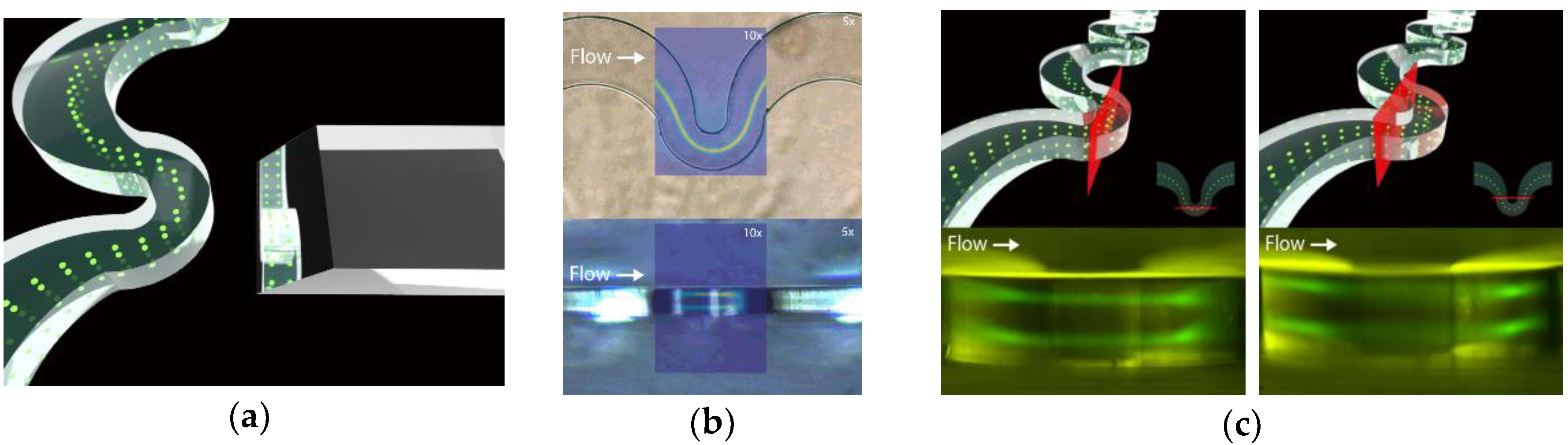
In order to test the suitability of our simulation model, a microfluidic device with the same serpentine geometry was created employing conventional photolithography techniques. SU8 (SU8-2150, MicroChem Corp., Newton, MA, USA) was spun on a 3-inche silicon wafer at 3500 RPM to obtain the desired channel height. The design of the serpentine was transferred from a chromium mask onto the SU8 layer using a UV mask aligner (MG 1410, SÜSS MicroTec AG, Garching, Germany). The microfluidic chip was elaborated in polydimethylsiloxane (PDMS) (Sylgard 184 from Dow Corning Corp., Midland, MI, USA). In addition to the conventional channels, the PDMS device also incorporated cavities to insert micromachined glass mirrors in the vicinity of the serpentine. The PDMS cavities devoted to the mirror had to be casted from micromachined structures directly stuck onto the Si wafer and placed very close to the fluidic channel. The mirrors were oriented at 45° and its field of view covered the entire height of the fluidic channel. This allowed to visualize the two stable trajectories of inertially focused fluorescent polystyrene particles (Figure 1).
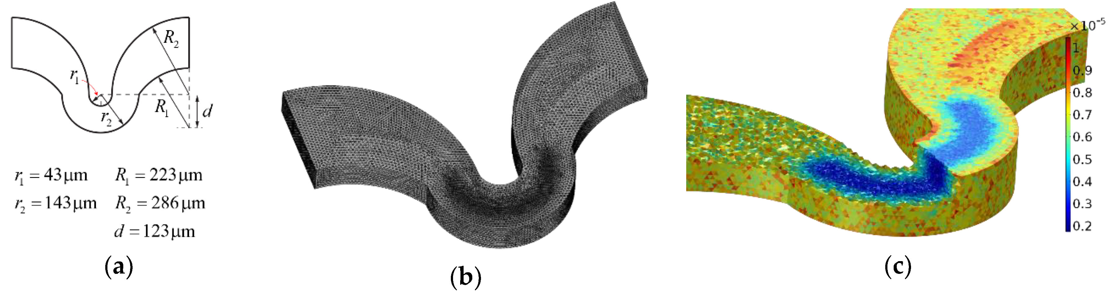
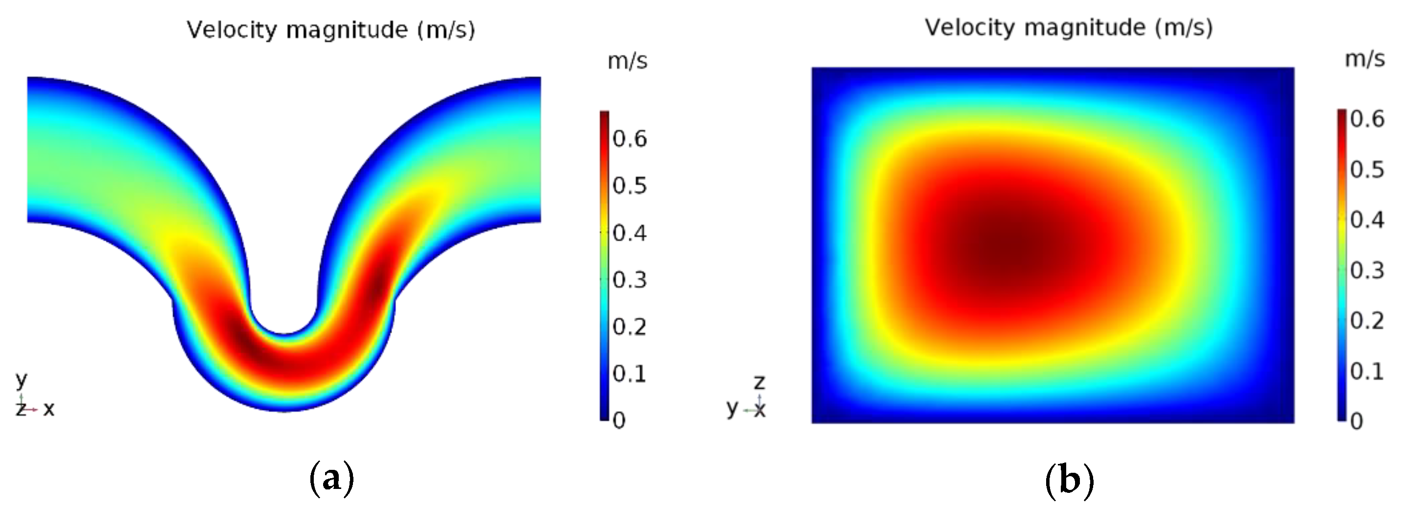
For simulation involving only the fluid, which was used to find the solution for the transverse flow, a 3D periodic unit of the serpentine (Figure 2) was used as the computational domain. Periodic flow conditions were required to set a pressure difference between a source boundary, where the fluid enters the domain, and a destination group through which the fluid exits the domain. The pressure difference was set at 857 Pa so that the desired flow rate of 130 μL/min was obtained during the simulation; the same used in the experiment with the fluidic device. We chose this geometry and flow rate for the simulation because the experimental results showed very good focusing conditions for particles that were optimal after 24 big-small curve doublets. The mesh also incorporated a finer mesh region inside the small turn in order to improve the simulation results in the region around which Dean vortex centers are expected to develop. The governing equations for momentum and mass conservation solved during the computation step were:
ρ v t + ρ ( v ) v = [ p I + μ ( v + ( v ) T ) ]
ρ v = 0
where v is the velocity field of the flow, p the pressure, I the unit identity matrix, and ρ and μ the density and viscosity of the fluid, respectively.
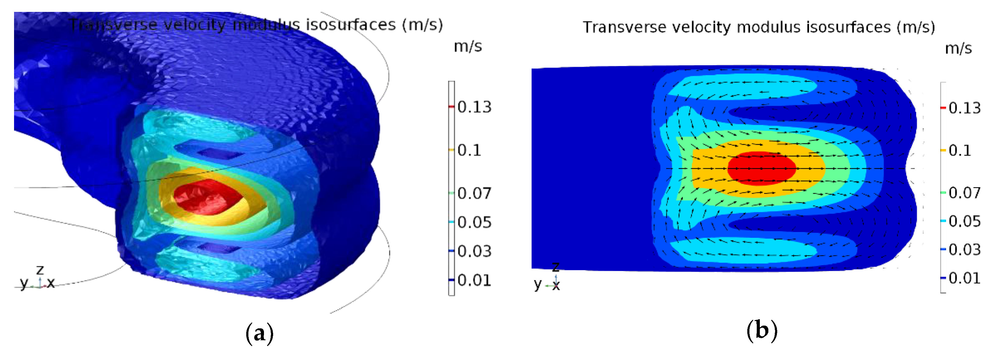
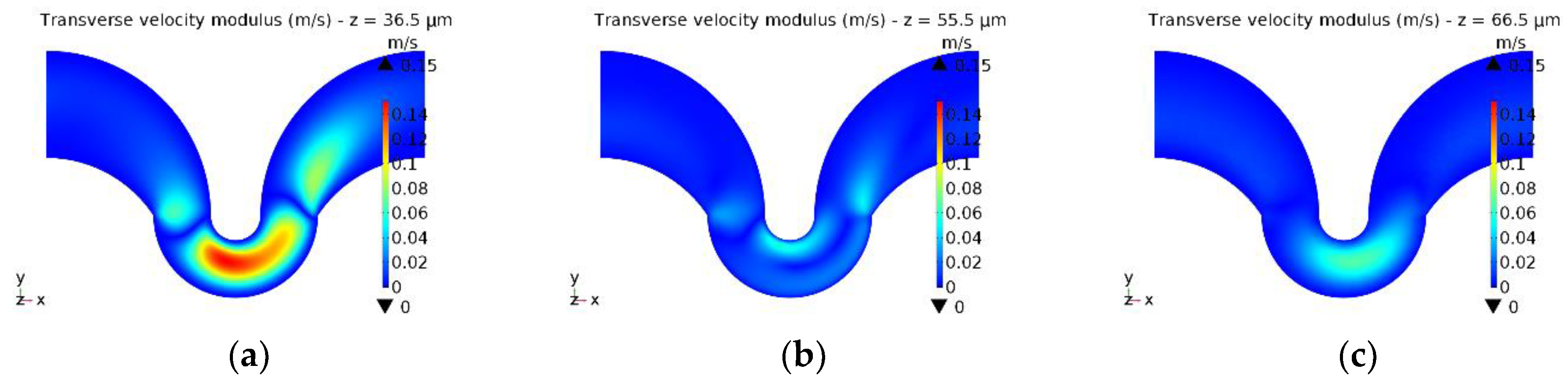
Bounded flows with some degree of curvature may facilitate the emergence of a flow field distribution that is perpendicular to the streamwise flow called Dean flow. These flows originate from the difference in velocity at the inner region of the fluidic channel with respect to the near-wall regions, which in comparison, due to the parabolic velocity profile, tend to be negligible. When the flow rate is sufficiently low, the viscosity between the flow elements in a moving mass of fluid suffices to force the streamlines of fluid to follow the curvature of the channel. The dimensionless parameter used to characterize the strength of transverse flows is the Dean number, D e = R e D h / 2 r ; where D h = 2 w h / w + h is the hydraulic diameter, where w and h are the width and height of the channel, respectively, and r is the radius of the curved channel.
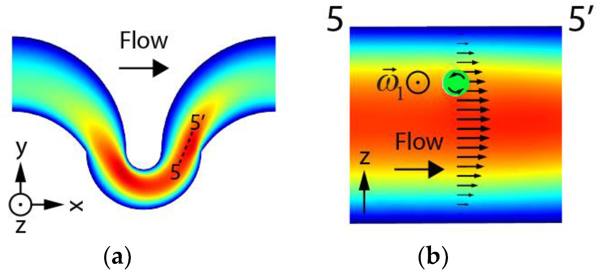
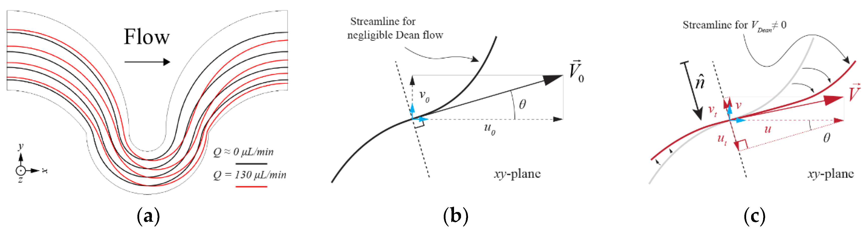
We propose a new approach by which the direction and magnitude of Dean flows can be numerically calculated at the pointwise level inside a simulation domain employing a FEM. The flow field is simulated at low and high flow rates and the differences between them are measured point-by-point in order to infer the magnitude and direction of the resulting transverse (Dean) flow. In our calculations, we chose the transverse components of the flow field at a given point to be the velocity field in the z direction (w), and the velocity field components in the x-y plane (u and v for x and y components, respectively). The latter coordinates are projected along a direction perpendicular to the streamlines obtained for the simulation at low flow rates (Figure 3). This method can be applied to any channel geometry, provided that the solutions for two different regimes, creeping flow, and regular laminar flow, can be obtained.
The analytical expression of the transverse flow field is then defined point-by-point and expressed in terms of the variables obtained in a simulation involving a low flow rate (Q(v0 = 1 μm/s) ≈ 1.8 × 10⁻⁴ μL/min), u0 and v0, and the variables obtained in the studied flow rate (Q(v0 = 0.67 m/s) = 130 μL/min) u, v and w:
v trans = ( u sin θ v cos θ ) n + w z ;   θ = tan 1 ( v 0 u 0 ) .
Dean patterns are commonly represented as flow field projections in a section of a microfluidic channel [26,34,45,46]. Such representation is indirectly based on the assumption that the streamlines of a hypothetical creeping flow are perpendicular to the said plane because its tangent components are taken as the Dean flow components. Reference cross-sectional planes (based on the geometry of the channel) to represent such flows can yield inaccurate results since, in general, it cannot be guaranteed that the streamlines of a flow, for which inertial effects can be neglected, are indeed perpendicular to the reference plane at any point. This is particularly true for the case of channels with complex geometries, such as serpentines or mixers, where new techniques have to be applied in order to visualize the complicated flow patterns that emerge [47,48].
The FSI simulation (in addition to N-S equations) also incorporated a term for the load on the solid boundary and a moving wall condition (displacement of the solid) for the fluid domain:
F solid = n ^ [ p I + μ ( v + ( v ) T ) ]
v wall = u solid t
were n ^ is the normal vector to the boundary of the sphere, v wall is the velocity of the fluid-solid interface, which acts as a moving wall for the fluid, and u solid is the structural displacement of the solid.
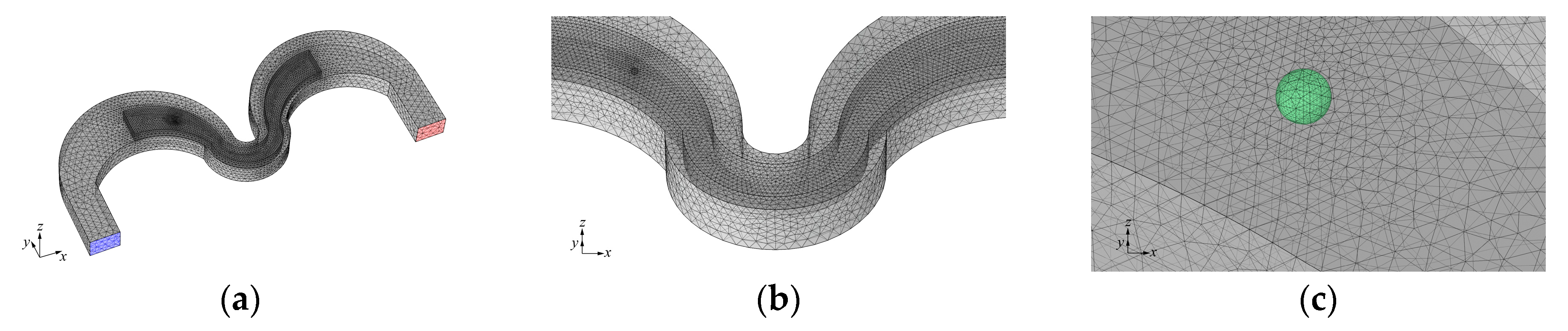
Figure 4 depicts the 3D fluid domain employed during the FSI simulation process. Unlike the stationary case, we opted not to use a periodic domain in the simulation involving the interaction between the particle and the flow. The reason is that periodic flow conditions only allow the use of pressure differences between the source and destination boundaries of the domain. The problem of using a pressure difference as a driving source for the flow in a transient simulation is that the pressure difference between the source and the destination boundaries—the pressure needed to obtain the desired flow rate—fixes the time it takes the flow to achieve stationary conditions, a regime that is expected as the particle travels through the region of interest (the small curve). Unfortunately, in our geometry, the time it takes the flow to achieve such conditions is so long that the particle penetrates the region of interest, while the flow hasn’t yet achieved stationary conditions (stationary flow rate and velocity profiles). Instead, by fixing an inflow velocity field distribution as a boundary condition for the inlet modulated by a smooth time dependent function, we can artificially set the time it takes the fluid domain to achieve a fully developed flow, a time that will be short enough so that the particle enters the small turn long after this condition is achieved. With this new boundary condition, we designed a new domain that comprised of a straight channel section, where the flow first develops, followed by a succession of big-small-big turns whose geometric parameters coincide with the microfluidic chip used to focus Ø = 10 μm particles in the experimental section. Like in the CFD simulation, the flow rate was set at 130 μL/min. The inlet velocity flow profile is approximated to that of a rectangular section channel by the expression:
v ( r , t ) = 16 v 0 x ( x 0 x ) z ( z 0 z ) x 0 2 z 0 2 step ( t [ 1 s ] ) y ^
where step (t[1/s]) is a dimensionless smoothed step function included to improve the convergence at the beginning of the time dependent simulation. 16 / x 0 2 z 0 2 is a normalizing factor at the inlet boundary condition so that v ( r , t ) = v 0 at the center of the inlet. Similarly, the expression in the numerator ensures that v ( r , t ) decays from the center of the channel out down to 0 at the walls in accordance with the no slip wall boundary condition for the flow introduced in the simulation. Notice that in the selected reference frame v ( r , t ) has only a y-component at the inlet (Figure 4a). A 0 Pa pressure condition is set at the outlet. v 0 is chosen so that, after stationary conditions are achieved, the desired flow rate is obtained in the channel (with our channel section, Q(v0 = 0.74 m/s) ≈ 130 μL/min). The flow rate is monitored by integrating the obtained flow fields across an arbitrary section of the channel. The length of the straight section ensures that the approximated velocity profile will have enough time to be fully developed at its end, before entering the first of the two big turns. Likewise, the big turn was completely included in the computational domain to ensure that the developed flow at the entry of the small turn was as similar as possible to the periodic case.
The mesh of the fluid domain was composed of two differentiated regions with two different mesh sizes (Figure 4b). The finer mesh region was restricted to the upper half of the channel. It was devoted to act as an “envelope” domain for a particle in the upper stable trajectory; it was placed in such a way that, during the simulations, the particle would remain inside this domain at all times. The finer mesh allows the solver to calculate the variables of the problem more precisely, since it can resolve the gradients of pressure and velocity in the vicinity of the sphere more reliably. The domain also included a spherical mesh 10 μm in diameter (Figure 4c), representing a particle, whose material properties were adjusted to match those of polystyrene. The series of FSI simulations consisted of numerically solving pathline trajectories of these spherical particles with different initial positions. The initial and final positions in the resulting simulation were located well away from the entry and exit of the small turn of the serpentine so that the particle’s behavior in this region was entirely captured. The mesh of the sphere itself was customized with lower element sizes than the predefined ones in order to obtain a reliable measurement of the calculated reaction forces.
Since the flow and pressure profiles solutions are symmetric in z, the study of one of the two trajectories is enough to characterize the effects of the Dean flow when no interaction between particles is considered. In order to reduce the computational complexity and the number of degrees of freedom of the simulation, a coarser mesh was used in the rest of the fluid domain, a domain which only contained fluid throughout the simulation. It has to be stressed that due to the geometry of the problem and the complexity of the flow patterns arising in the channel, the 3D simulation could not make use of symmetries that would speed up the convergence of the solutions. Likewise, inertial terms in the N-S equations (which lead to non-linearities) could not be neglected in order for inertial migration effects to arise in the solutions.
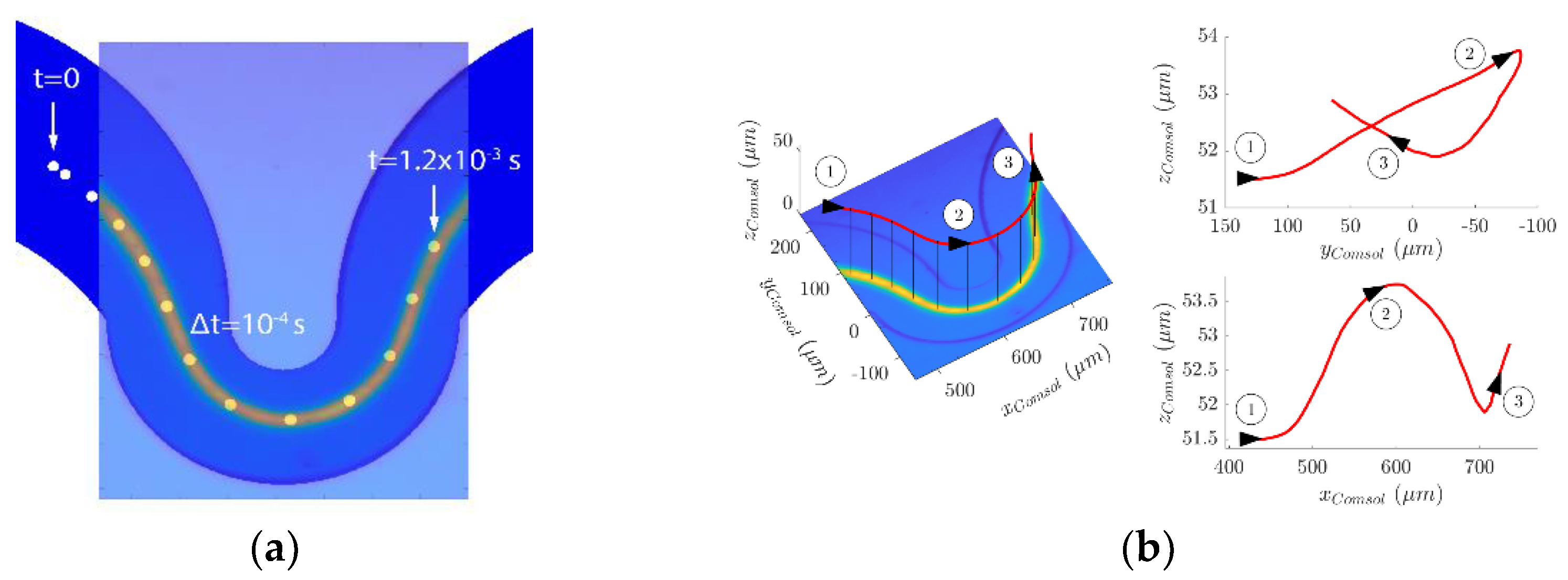
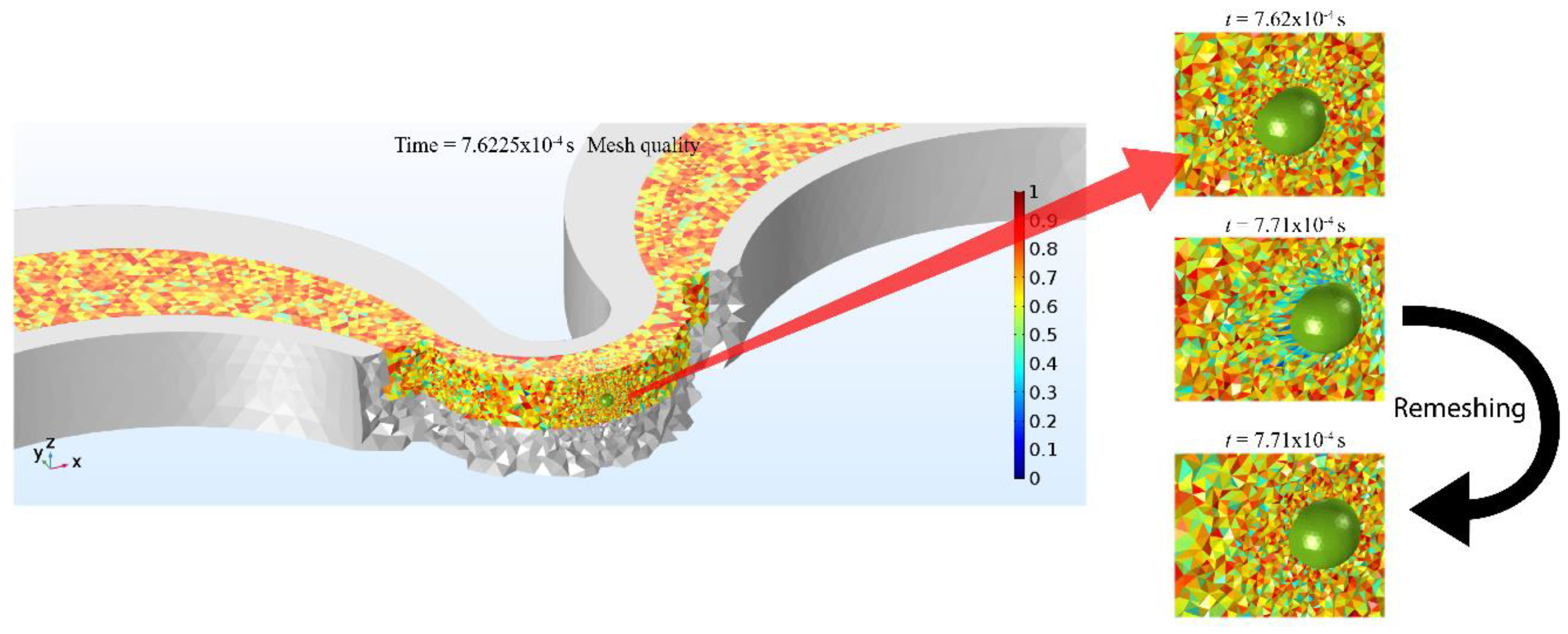
In our problem, the FSI formulation couples the flow field and pressure solutions from N-S equations for an incompressible flow to solid mechanics equations, namely, the reaction forces over the solid boundary of the particle. The use of the FSI formulation for the time-dependent study in COMSOL (version 5.0, COMSOL Inc., Stockholm, Sweden) incorporates an arbitrary Lagrangian-Eulerian (ALE) method that takes into account the deformation of the mesh in the fluid domain caused by the movement of the particle being displaced under the influence of the surrounding flow. No constraint is applied on the particle, so it becomes a freely moving mesh. This circumstance imposes the use of an automatic remeshing feature at the mesh surrounding the particle, otherwise the fluid domain would be deformed indefinitely over time as the particle (the spherical mesh) moves along the channel (Figure 5).

3. Results and Discussion

3.1. Stationary Solution for the Transverse Flow Field

Figure 6 illustrates the simulation results for the velocity magnitudes of the flow at a given flow rate and channel height (Q = 130 μL/min, h = 73 μm). The velocity magnitude distribution clearly reveals the asymmetric character of the flow; the maximum values of the velocity tend to be displaced in the streamwise direction.
The transverse flow was decoupled from the main flow so the contribution of the Dean vortices can be inferred (Figure 7). In order to get a complete picture and to improve the understanding of the geometric complexity of the transverse flows, transverse velocity isosurfaces are also represented in Figure 8. As expected, secondary flows direction and intensities vary along the height of the small curve having its maximum intensity in the middle height region of the channel (corresponding to flow moving radially outwards) and in opposite direction near the top and bottom boundaries (flow moving inwards). No secondary Dean vortices were observed in the simulations of the small curve given their moderate aspect ratio [49]. For heights near the middle of the channel, two well-defined boundaries of negligible transverse flow between the small and big turns regions are visible. These boundaries are the consequence of a flow transition in these regions due to a rotation inversion of the Dean vortices between the small and big turns. For a region between the half height of the channel and its top wall (z = 55.5 μm), a curved path with negligible transverse flow velocity is visible at the inner region of the small turn (Figure 7b). At z = 17.5 μm, an additional null velocity path can be found. These paths, which follow the curvature of the small turn, represent the position of the center of the upper and lower Dean vortices generated in the small turn (Figure 8). Some authors have highlighted what appears to be a tendency of focused particles to travel along vortices centerlines [34], which would explain the emergence of two stable trajectories of focused particles in some curved geometries, one for each upper and lower Dean vortices centerlines.

3.2. FSI Simulation

One of the purposes of the FSI simulation was to find the numerical solution that would best describe the movement of a Ø = 10 μm particle along the trajectory found in the experimental section at Q = 130 μL/min. An overlap between the averaged fluorescence streak image from the experiment and an animation provided by the time dependent solution of the moving sphere was used as a comparison method between the experiment and the simulation (Figure 9). Since no height information of the particles can be extracted from a zenithal view of the fluorescence streak, lateral images of the small curve were taken using the inserted mirrors in the microfluidic device. This allowed to obtain the approximate height of the trajectory and use it as a guess for the particles’ initial position in the simulation. Since the height of the stream of particles could not be measured with enough precision, slightly different initial positions for the spherical mesh were tested during the FSI simulations in order to find the best fit with the experimental data.

3.3. Particle Rotational Velocity Components

Data from the FSI simulation was analyzed to obtain the angular velocity components of the particle as it moves along its trajectory in the upper half region of the small curve (Figure 10a) under the influence of the upper Dean vortex. Given the observed changes in the direction and strength of the angular velocity vector in this region of the channel, we can distinguish between different particle behavior regimes (Figure 10b–d). The obtained rotation rates are in the kilohertz range, the same that has been observed in straight channels with conventional flow rates [21,50].
The particle, initially at rest at the beginning of the simulation, gradually starts to spin while being displaced by the drag in the streamwise direction producing an angular velocity vector contained in the x-y plane (Section 1 in Figure 10b and Figure 11). Taking into account its proximity to the upper wall, the spin direction of the particle is the one that might be expected for an inertially focused particle under the influence of a vertical parabolic shear gradient [22,23]. Viscous forces exerted by the fluid located between the particle and the inner region of the channel (which moves faster than the particle) and the fluid between the particle and the upper wall (moving slower than the particle) create a torque that add up to the same direction, creating a net spin over the particle (ω1).
Right after entering the small curve, the angular velocity vector momentarily deviates downwards, indicating the emergence of a clockwise spin rotation around the z axis (if we look at the particle from above). This component reaches its maximum in the transition boundary between the inward and outward lateral moving flow (Section 2 in Figure 10b and Figure 12a,b) at the plane where the particle is moving. Once the particle leaves this region, the velocity vector returns to the x-y plane.
In the next region of the trajectory, as the particle approximates halfway of the small turn, the influence of the upper Dean vortex starts to show up as the particle is forced to rotate in the direction of the Dean vortex [34]. As for the total angular velocity vector of the sphere, it gradually moves counterclockwise (Section 2 and Section 3 in Figure 10b) under the influence of this new component. Since the particle translates along the centerline of the Dean vortices, the flow revolving around the particle (a flow that is perpendicular to the streamwise flow) forces it to acquire an angular velocity component tangent to its trajectory pointing upstream (Figure 12c) along the regions where Dean flows are stronger. This is reflected by the fact that the resulting angular velocity vector is no longer perpendicular to the trajectory (Section 3 in Figure 10b). A side-effect of the rotation of the particle due to the shear gradient (causing a strong ω1 component), while being under the influence of a secondary flow, is that the interface between the outward- and inward-moving flow suffers a distortion caused by the no-slip boundary condition of the rotating particle; the surface of the rotating sphere drags the surrounding fluid altering this interface. This distortion causes the torque to suffer a change on its balance that causes the velocity vector to move downwards (Figure 12d), increasing its negative z-component (clockwise rotation of the particle as seen from above).
Simultaneously, as the particle moves along the curve and this clockwise rotation in the z direction increases in magnitude, it further induces a distortion of the Dean flow in the z direction around the particle modifying the torque balance again (Figure 13).
This additional distortion modifies the angular velocity vector by forcing it to move inwards to the center of curvature (Section 3 in Figure 10b). Apparently, this induced torque is strong enough to counteract the effect of the shear-induced ω1 component, inverting its original spin direction.
As the particle approaches the end of the small curve, the strength of the Dean flow gradually decreases and the distortions of the flow are greatly attenuated. As can be seen in Figure 14b, the interface between the inward- and outwards-moving flow remains relatively unaltered. However, similarly to what is observed at the inlet of the small curve, the gradients that the particle encounters as it exits the small curve induce a strong counterclockwise rotation around the z-axis (Figure 14c).
At the outlet of the small curve, the particle also encounters regions with big velocity magnitudes, hence, stronger gradients in the vertical direction. The cumulative effect of the reduction in Dean intensity and the pronounced streamwise flow gradient increase in the vertical direction causes a restitution of the original particle spin pointing outwards (Figure 15, Section 4 in Figure 10b). Like in the case of the particle entering the small curve: since the particle is moving far from the lateral walls, the shear-induced rotation effect is expected to be stronger in the vertical direction; because of the parabolic velocity profile, the lagging-leading flow differences at each side of the particle are expected to be much greater in the vertical direction. As the particle enters the big curve, the angular velocity vector gradually moves to the x-y plane again.

4. Conclusions

We presented CFD and FSI simulation results for the flow in an asymmetric serpentine and an unrestricted free spherical particle. A custom-made microfluidic device was fabricated in order to compare the numerical results with the experiment conducted at the same conditions. The micro-mirrors inserted in the microfluidic device were useful to verify the existence of two stable trajectories, mirrored in z, for the focused particles and to make an estimation of the height of the streak to use it as the initial conditions in the FSI time-dependent simulation.
We also introduced a new methodology, based entirely on the results of numerical simulations, to obtain the transverse flow magnitude in a curved geometry. The fact that this method is based on the measurable differences between a creeping flow and the flow containing transverse lateral flows helps find the direction and magnitude of the transverse flow at any point in the fluidic domain without any geometric bias such as the ones that may be introduced by section planes when Dean patterns are represented.
FSI results suggest that particles focused under inertial focusing conditions tend to be entrained in the centerlines of the Dean vortices, something already observed by Jiang et al. [34] with the IB-LBM method. This fact seems to be relativizing the importance of Dean drag contribution to inertial focusing conditions in curved channels; particles appear to have a preference to be focused at regions with small local lateral flow intensities. The comparison between the trajectory found in the simulation and the experimental one shows good agreement between them validating the join application of FSI + ALE + remeshing features in COMSOL.
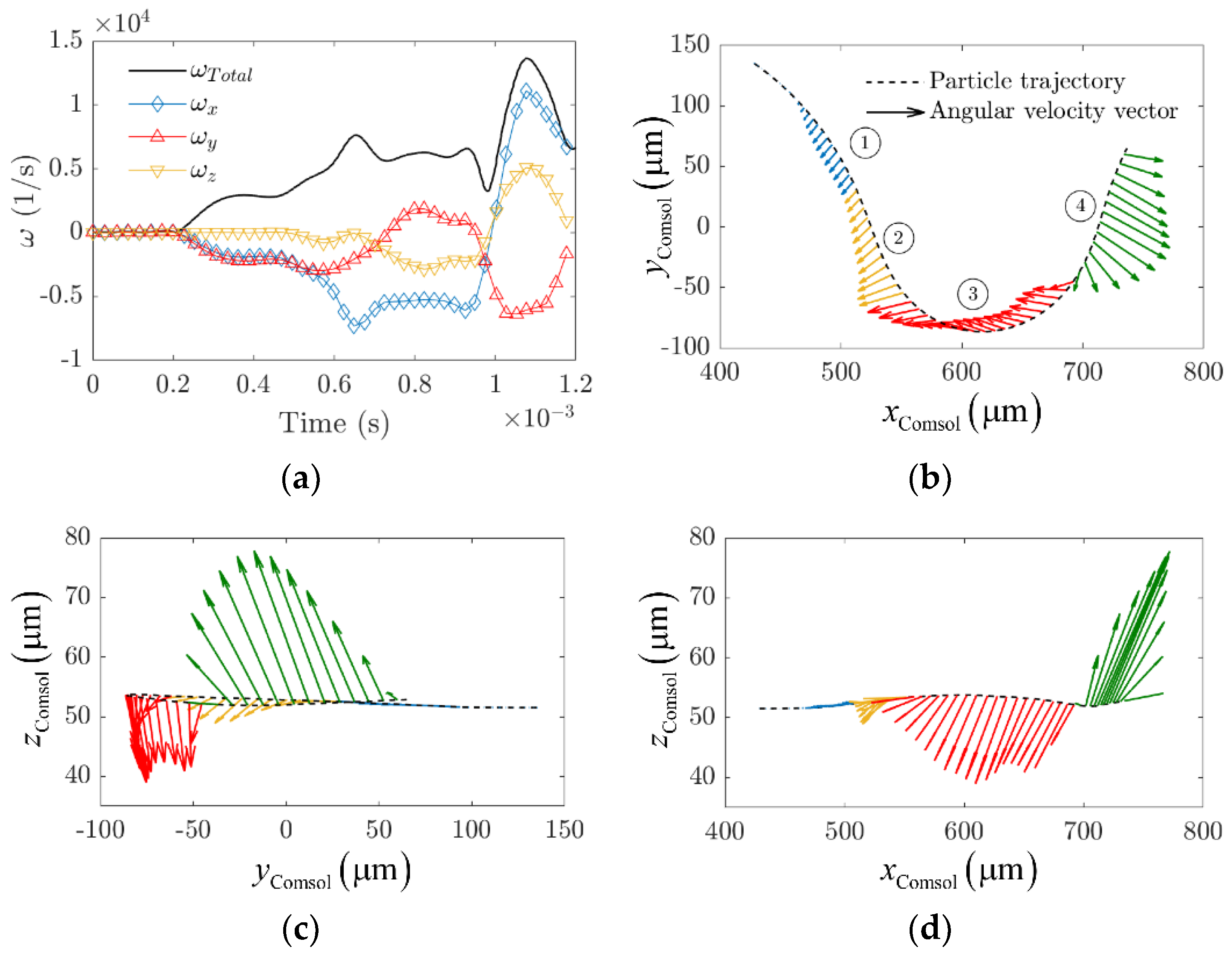
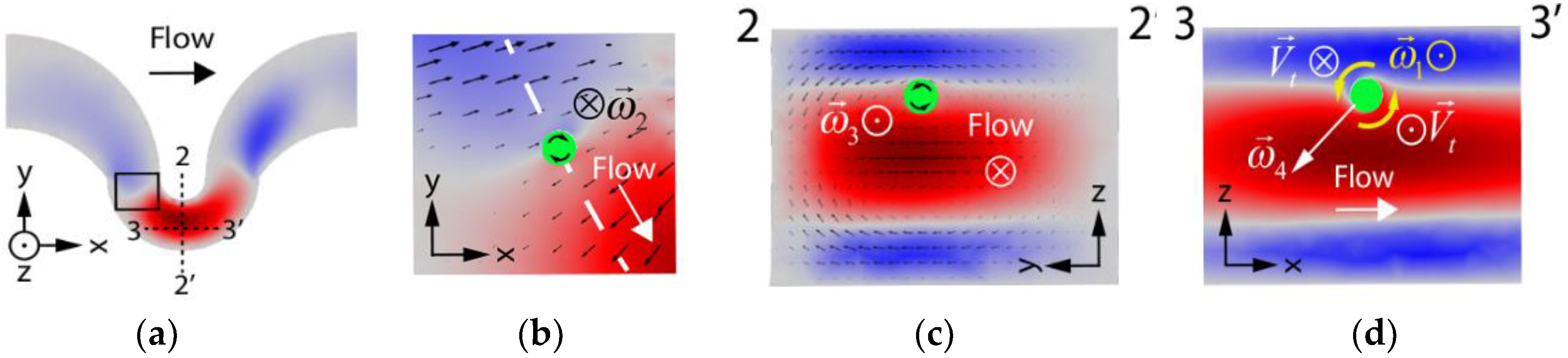
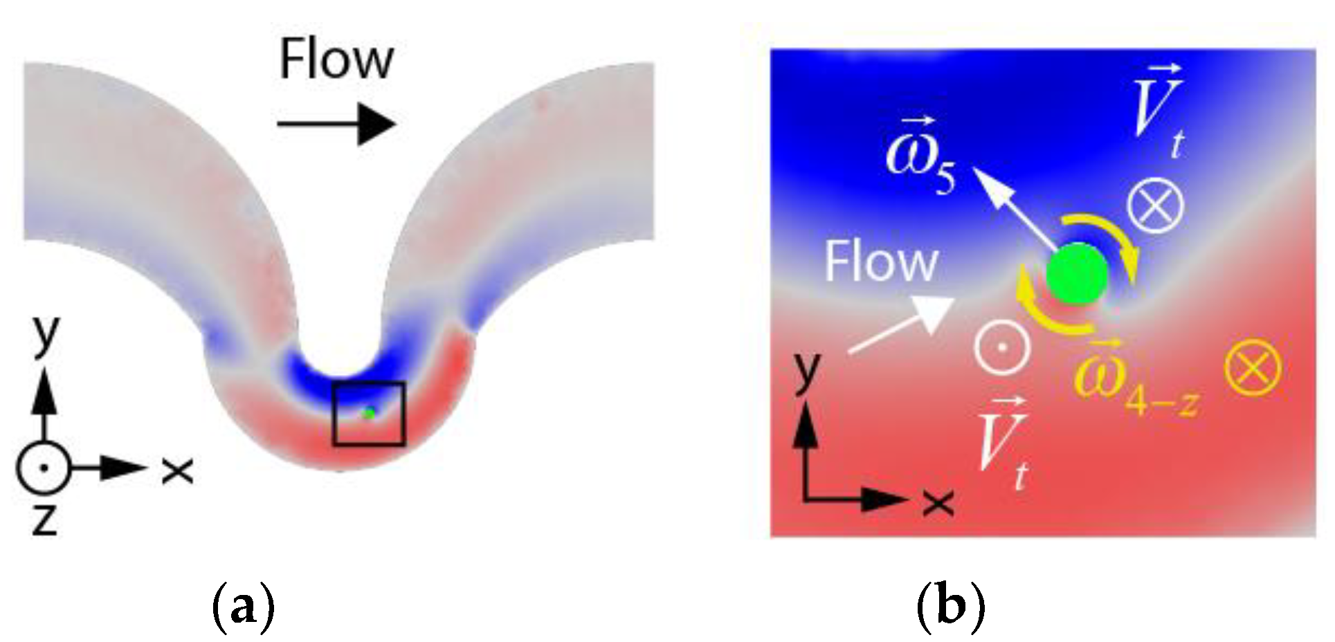
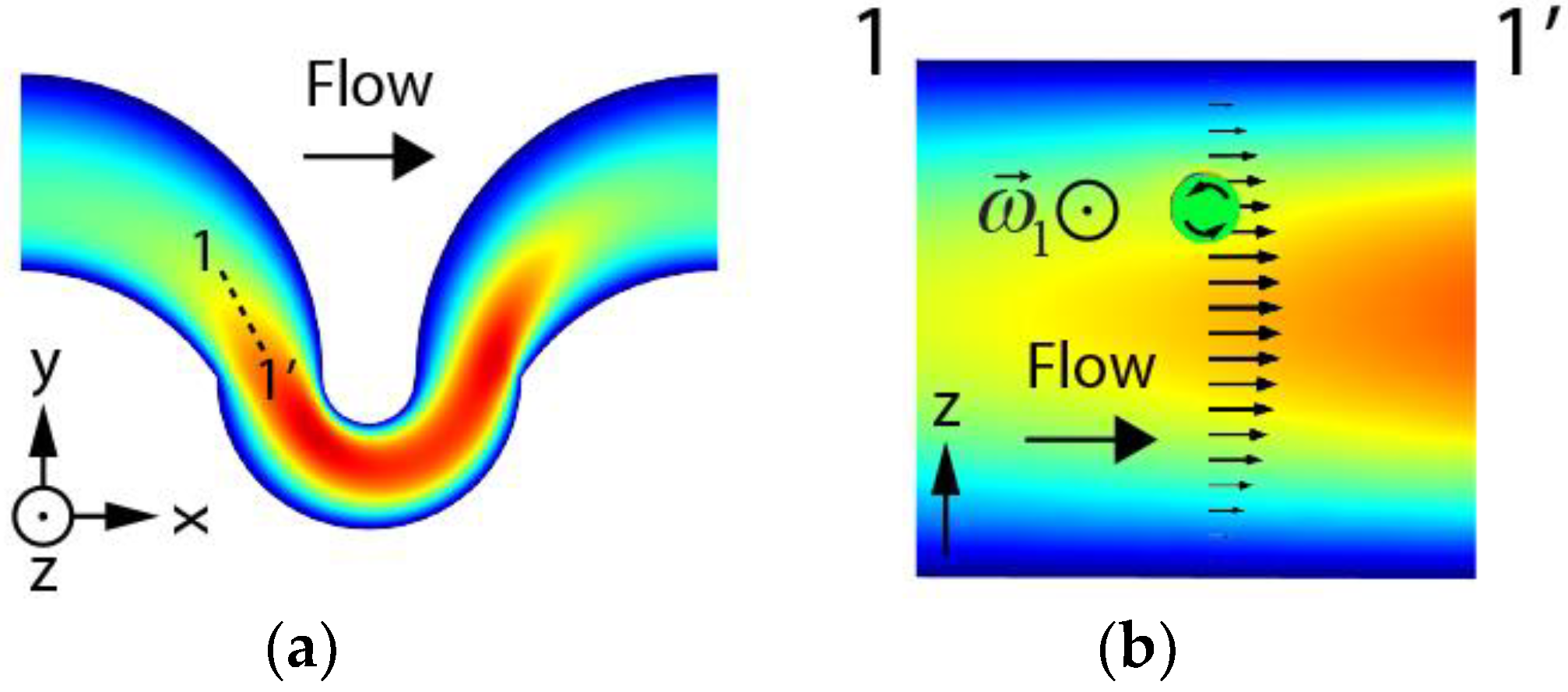
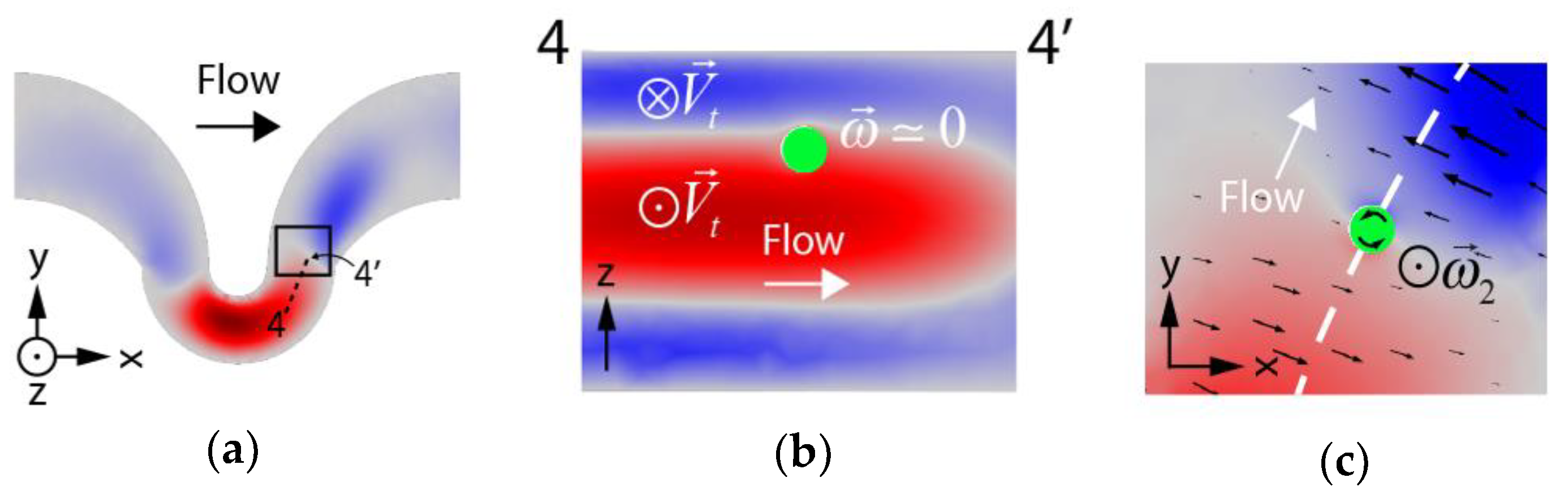
The obtention of the rotational components of the translating sphere revealed the complexity of the particle’s dynamics as it moves along its trajectory. This behavior clearly differs from the one observed in straight channels due to the presence of Dean flows in the small curve. Provided that particles seem to be translating along Dean vortices centerlines under focusing conditions, this fact can already be used as a simplification of the simulation by means of constrained variables because centerlines can be obtained with conventional CFD simulations alone. The elucidation of the theory behind the apparent movement and focusing of particles through vortices’ centerlines will require further studies (its response to flow rate changes and particle’s confinement ratio, among others). We believe that our analysis on angular velocity components can be incorporated to simpler simulation models to infer, at least as a first approximation, the evolution of the angular velocity of the particle on its path through a curved geometry, suppressing the need to perform computationally intensive simulations with coupled solvers. The use of a complex structure (the asymmetric serpentine) has probably improved our understanding of the particle’s behavior in a way that it probably couldn’t be achieved if we had simulated focusing conditions in a simpler geometry (a spiral or a curved channel for instance), for which Dean inversions and abrupt gradient changes hardly occur.

Author Contributions

Conceptualization, E.P.; Formal Analysis, E.P., J.M.; Funding Acquisition, M.A.; Investigation, E.P., J.M., F.D.; Methodology, E.P.; Project Administration, F.D., M.A.; Software, E.P.; Supervision, J.M., F.D.; Writing, E.P.

Funding

This research received financial support from Spanish Government under Project MAT2016-75716-C2-1-R (AEI/FEDER,UE) and TEC 2014-55948-R, and from Catalan Government under Project 2017 SGR 755 and 2014 SGR 1358.

Conflicts of Interest

The authors declare no conflict of interest.

References

  1. Poiseuille, J.L.M. Recherches sur les causes du mouvement du sang dans les vaisseaux capillaires. C. R. Acad. Sci. 1835, 6, 554–560. [Google Scholar]
  2. Tollert, H. Die Wirkung der Magnus-Kraft in laminaren Strömungen. Chem. Ing. Tech. 1954, 26, 141–150. [Google Scholar] [CrossRef]
  3. Taylor, M. The flow of blood in narrow tubes. Aust. J. Exp. Biol. 1955, 33, 1–16. [Google Scholar] [CrossRef]
  4. Maude, A.D.; Whitmore, R.L. The wall effect and the viscometry of suspensions. Br. J. Appl. Phys. 1956, 7, 98–102. [Google Scholar] [CrossRef]
  5. Saffman, P. On the motion of small spheroidal particles in a viscous liquid. J. Fluid Mech. 1956, 1, 540–553. [Google Scholar] [CrossRef]
  6. Di Carlo, D.; Irimia, D.; Tompkins, R.G.; Toner, M. Continuous inertial focusing, ordering, and separation of particles in microchannels. Proc. Natl. Acad. Sci. USA 2007, 104, 18892–18897. [Google Scholar] [CrossRef] [PubMed] [Green Version]
  7. Di Carlo, D.; Edd, J.F.; Irimia, D.; Tompkins, R.G.; Toner, M. Equilibrium separation and filtration of particles using differential inertial focusing. Anal. Chem. 2008, 80, 2204–2211. [Google Scholar] [CrossRef] [PubMed]
  8. Di Carlo, D. Inertial microfluidics. Lab Chip 2009, 9, 3038–3046. [Google Scholar] [CrossRef] [PubMed]
  9. Gossett, D.R.; Di Carlo, D. Particle focusing mechanisms in curving confined flows. Anal. Chem. 2009, 81, 8459–8465. [Google Scholar] [CrossRef] [PubMed]
  10. Kuntaegowdanahalli, S.S.; Bhagat, A.A.S.; Kumar, G.; Papautsky, I. Inertial microfluidics for continuous particle separation in spiral microchannels. Lab Chip 2009, 9, 2973–2980. [Google Scholar] [CrossRef] [PubMed]
  11. Oakey, J.; Applegate, R.W.; Arellano, E.; Di Carlo, D.; Graves, S.W.; Toner, M. Particle focusing in staged inertial microfluidic devices for flow cytometry. Anal. Chem. 2010, 82, 3862–3867. [Google Scholar] [CrossRef] [PubMed]
  12. Martel, J.M.; Toner, M. Inertial focusing dynamics in spiral microchannels. Phys. Fluids 2012, 24, 032001. [Google Scholar] [CrossRef] [PubMed] [Green Version]
  13. Sun, J.; Li, M.; Liu, C.; Zhang, Y.; Liu, D.; Liu, W.; Hu, G.; Jiang, X. Double spiral microchannel for label-free tumor cell separation and enrichment. Lab Chip 2012, 12, 3952–3960. [Google Scholar] [CrossRef] [PubMed] [Green Version]
  14. Cox, R.G.; Brenner, H. The lateral migration of solid particles in Poiseuille flow—I theory. Chem. Eng. Sci. 1968, 23, 147–173. [Google Scholar] [CrossRef]
  15. Ho, B.P.; Leal, L.G. Inertial migration of rigid spheres in two-dimensional unidirectional flows. J. Fluid Mech. 1974, 65, 365–400. [Google Scholar] [CrossRef]
  16. Vasseur, P.; Cox, R.G. The lateral migration of a spherical particle in two-dimensional shear flows. J. Fluid Mech. 1976, 78, 385–413. [Google Scholar] [CrossRef]
  17. Asmolov, E.S. The inertial lift on a spherical particle in a plane Poiseuille flow at large channel Reynolds number. J. Fluid Mech. 1999, 381, 63–87. [Google Scholar] [CrossRef]
  18. Subramanian, G.; Koch, D.L. Inertial effects on the transfer of heat or mass from neutrally buoyant spheres in a steady linear velocity field. Phys. Fluids 2006, 18, 073302. [Google Scholar] [CrossRef]
  19. Yang, C.; Zhang, J.; Koch, D.L.; Yin, X. Mass/heat transfer from a neutrally buoyant sphere in simple shear flow at finite Reynolds and Peclet numbers. AIChE J. 2011, 15, 1419–1433. [Google Scholar] [CrossRef]
  20. Hood, K.; Lee, S.; Roper, M. Inertial migration of a rigid sphere in three-dimensional Poiseuille flow. J. Fluid Mech. 2015, 765, 452–479. [Google Scholar] [CrossRef] [Green Version]
  21. Di Carlo, D.; Edd, J.F.; Humphry, K.J.; Stone, H.A.; Toner, M. Particle segregation and dynamics in confined flows. Phys. Rev. Lett. 2009, 109, 094503. [Google Scholar] [CrossRef] [PubMed]
  22. Amini, H.; Sollier, E.; Weaver, W.M.; Di Carlo, D. Intrinsic particle-induced lateral transport in microchannels. Proc. Natl. Acad. Sci. USA 2012, 109, 11593–11598. [Google Scholar] [CrossRef] [PubMed] [Green Version]
  23. Lee, W.; Amini, H.; Stone, H.A.; Di Carlo, D. Microfluidic crystals: Self-assembly and control of particle streams. Proc. Natl. Acad. Sci. USA 2010, 107, 22413–22418. [Google Scholar] [CrossRef] [PubMed]
  24. Wang, Q.; Yuan, D.; Li, W. Analysis of hydrodynamic mechanism on particles focusing in micro-channel flows. Micromachines 2017, 8, 197. [Google Scholar] [CrossRef]
  25. Liu, C.; Hu, G.; Jiang, X.; Sun, J. Inertial focusing of spherical particles in rectangular microchannels over a wide range of Reynolds numbers. Lab Chip 2015, 15, 1168–1177. [Google Scholar] [CrossRef] [PubMed] [Green Version]
  26. Liu, C.; Xue, C.; Sun, J.; Hu, G. A generalized formula for inertial lift on a sphere in microchannels. Lab Chip 2016, 16, 884–892. [Google Scholar] [CrossRef] [PubMed] [Green Version]
  27. Ladd, A.J.C. Numerical simultaions of particulate suspensions via a discretized Boltzmann equation. Part 1. Theoretical foundation. J. Fluid Mech. 1994, 271, 285–309. [Google Scholar] [CrossRef]
  28. Ladd, A.J.C. Numerical simultaions of particulate suspensions via a discretized Boltzmann equation. Part 2. Numerical results. J. Fluid Mech. 1994, 271, 311–339. [Google Scholar] [CrossRef]
  29. Ladd, A.J.C.; Verberg, R. Lattice-Boltzmann simulations of particle-fluid suspensions. J. Stat. Phys. 2001, 104, 1191–1251. [Google Scholar] [CrossRef]
  30. Yi, H. The lift on a spherical particle in rectangular pipe flow. Chin. J. Phys. 2013, 52, 174–184. [Google Scholar] [CrossRef]
  31. Kandhai, D.; Vidal, D.J.-E.; Hoekstra, A.G.; Hoefsloot, H.; Iedema, P.; Sloot, P.M.A. Lattice-Boltzmann and finite element simulations of fluid flow in a SMRX static mixer reactor. Int. J. Numer. Methods Fluids 1999, 31, 1019–1033. [Google Scholar] [CrossRef]
  32. Feng, Z.-G.; Michaelides, E.E. The immersed boundary-lattice Boltzmann method for solving fluid-particles interaction problems. J. Comput. Phys. 2004, 195, 602–628. [Google Scholar] [CrossRef]
  33. Peskin, C.S. The immersed boundary method. Acta Numer. 2002, 11, 479–517. [Google Scholar] [CrossRef]
  34. Jiang, D.; Tang, W.; Xiang, N.; Ni, Z. Numerical simulation of particle focusing in symmetrical serpentine microchannel. RSC Adv. 2016, 6, 57647–57657. [Google Scholar] [CrossRef]
  35. Le Tallec, P.; Gerbeau, J.-F.; Hauret, P.; Vidrascu, M. Fluid structure interaction problems in large deformation. C. R. Mec. 2005, 333, 910–922. [Google Scholar] [CrossRef] [Green Version]
  36. Wall, W.A.; Gerstenberger, A.; Gamnitzer, P.; Förster, C.; Ramm, E. Large Deformation Fluid-Structure Interaction—Advances in ALE Methods and New Fixed Grid Approaches; Springer: Berlin/Heidelberg, Germany, 2006; pp. 195–232. ISBN 978-3-540-34596-1. [Google Scholar]
  37. Bak, S.; Yoo, J.; Song, C.Y. Fluid-structure interaction analysis of deformation of sail of 30-foot yacht. Int. J. Naval Archit. Ocean Eng. 2013, 5, 263–276. [Google Scholar] [CrossRef]
  38. Tian, F.-B.; Dai, H.; Luo, H.; Doyle, J.F.; Rousseau, B. Fluid-structure interaction involving large deformations: 3D simulations and applications to biological systems. J. Comput. Phys. 2014, 258, 451–469. [Google Scholar] [CrossRef] [PubMed]
  39. Dubini, G.; Pietrabissa, R.; Montevecchi, F.M. Fluid-structure interaction problems in bio-fluid mechanics: A numerical study of the motion of an isolated particle freely suspended in channel flow. Med. Eng. Phys. 1995, 17, 609–617. [Google Scholar] [CrossRef]
  40. Barreiro, A.; Crespo, A.J.C.; Domínguez, J.M.; Gómez-Gesteira, M. Smoothed particle hydrodynamics applied in fluid structure interactions. WIT Trans. Built Environ. 2013, 129, 75–84. [Google Scholar] [CrossRef]
  41. He, Y.; Bayly, A.E.; Hassanpour, A. Coupling CFD-DEM with dynamic meshing: A new approach for fluid-structure interaction in particle-fluid flows. Powder Technol. 2018, 325, 620–631. [Google Scholar] [CrossRef] [Green Version]
  42. Warkiani, M.E.; Guan, G.; Luan, K.B.; Lee, W.C.; Bhagat, A.A.; Chaudhuri, P.K.; Tan, D.S.; Lim, W.T.; Lee, S.C.; Chen, P.C.; et al. Slanted spiral microfluidics for the ultra-fast, label-free isolation of circulating tumor cells. Lab Chip 2014, 14, 128–137. [Google Scholar] [CrossRef] [PubMed] [Green Version]
  43. Kim, T.H.; Yoon, H.J.; Stella, P.; Nagrath, S. Cascaded spiral microfluidic device for deterministic and high purity continuous separation of circulating tumor cells. Biomicrofluidics 2014, 8, 064117. [Google Scholar] [CrossRef] [PubMed] [Green Version]
  44. Zhang, J.; Yan, S.; Li, W.; Alici, G.; Nguyen, N.-T. High throughput extraction of plasma using a secondary flow-aided inertial microfluidic device. RSC Adv. 2014, 4, 33149–33159. [Google Scholar] [CrossRef]
  45. Zhou, J.; Kasper, S.; Papautsky, I. Enhanced size-dependent trapping of particles using microvortices. Microfluid. Nanofluid. 2013, 15, 611–623. [Google Scholar] [CrossRef] [PubMed] [Green Version]
  46. Javaid, M.U.; Cheema, T.A.; Park, C.W. Analysis of passive mixing in a serpentine microchannel with sinusoidal side walls. Micromachines 2018, 9, 8. [Google Scholar] [CrossRef]
  47. Rosaguti, N.R.; Fletcher, D.F.; Haynes, B.S. Laminar flow in a periodic serpentine channel. In Proceedings of the 15th Australasian Fluid Mechanics Conference, Sydney, Australia, 13–17 December 2004. [Google Scholar]
  48. Ahn, Y.-C.; Jung, W.; Chen, Z. Optical sectioning for microfluidics: Secondary flow and mixing in a meandering microchannel. Lab Chip 2008, 8, 125–133. [Google Scholar] [CrossRef] [PubMed]
  49. Nivedita, N.; Ligrani, P.; Papautsky, I. Evolution of secondary Dean vortices in spiral microchannels for cell separations. In Proceedings of the 17th International Conference on Miniaturized Systems for Chemistry and Life Sciences, Freiburg, Germany, 27–31 October 2013. [Google Scholar]
  50. Martel, J.M.; Toner, M. Inertial focusing in microfluidics. Annu. Rev. Biomed. Eng. 2014, 16, 371–396. [Google Scholar] [CrossRef] [PubMed]
Figure 1. (a) Render that illustrates the position of the lateral mirror with respect to the serpentine; (b) Zenithal (top) and lateral (bottom) views of the serpentine with an overlapped fluorescence streak image (false color) from inertially focused particles at a flow rate of 130 μL/min; (c) The limited depth of field of the employed objective allows the streak of particles reflected in the mirror to focus on different focus planes (red planes).
Fluids 03 00062 g001
Figure 2. (a) Geometry’s dimensions of the serpentine; (b) meshed simulation domain for the CFD simulation represented as a periodic unit of the serpentine. The channel is 73 μm in height; (c) inner region of the simulation domain. Part of the mesh has been removed to expose the insides of the mesh, emphasizing the effects of the finer mesh regions in the small curve. Color scale (μm) represents the mesh element size.
Fluids 03 00062 g002
Figure 3. (a) Obtained streamlines for a flow with negligible Dean flow (black lines) and for Q = 130 μL/min (red lines) for h = 73 μm measured at z = 36.5 μm. Dean flows at this height displace the streamlines outwards in the central region of the curves; (b) decomposition, at any given point, of a flow velocity vector ( v ) to a direction perpendicular to its corresponding negligible Dean flow streamline at that point. The perpendicular direction ( n ^ ) is found using the variables u0 and v0 from the solution at low flow rates; (c) once the flow rate is increased, Dean flow appears and the velocity vector, now with v and u components, can be projected along vector n ^ .
Fluids 03 00062 g003
Figure 4. (a) Meshed simulation domain for the FSI simulation. The fluid enters the domain through one of the straight section ends (blue surface) and exits through the other side (red surface); (b) detail of the different sized meshes. The upper one corresponds to the region of the domain where the particle will translate through the curve; (c) zoomed section of the mesh showing the particle domain (green) at its initial position inside the channel.
Fluids 03 00062 g004
Figure 5. Different stages of the movement of a Ø = 10 μm spherical domain (green sphere) through the fine (rainbow) mesh. The last picture shows the remeshing of the fine mesh. Bluish facets in the fine mesh represent low mesh quality regions.
Fluids 03 00062 g005
Figure 6. (a) Flow velocity magnitude for Q = 130 μL/min and h = 73 μm measured at z = 36.5 μm, at the middle height of the fluidic channel; (b) Flow velocity magnitude for the same flow conditions measured at the y-z plane halfway through the small curve.
Fluids 03 00062 g006
Figure 7. Modulus of the transverse flow field calculated at different heights. The transverse flow field strength is an order of magnitude weaker in the big curve. (a) At z = 36.5 μm (middle height), the magnitude for an outwards-moving flow is maximum; (b) At z = 55.5 μm, a null velocity region (the center of the upper Dean vortex) is visible in the central region of the small curve; (c) The magnitude of the velocity in the small curve increases again as we move upwards. This time, the flow is moving inwards, in the direction of the center of curvature.
Fluids 03 00062 g007
Figure 8. (a) Isosurfaces of the transverse velocity flow modulus cut through y-z plane; (b) Plane view of the cut section. The null transverse velocity paths are visible at the center of the Dean vortices.
Fluids 03 00062 g008
Figure 9. (a) Overlapping of the experimental image for a focused streak of Φ = 10 μm particles and positions of the particle calculated with the FSI simulation along the small (white circles). The overlapped image is represented in false color to improve the visibility of the streak; (b) Composed perspective of the 3D trajectory of the particle (red line).
Fluids 03 00062 g009
Figure 10. (a) Angular velocity components of the particle as a function of the simulation time. ωTotal is the total angular velocity magnitude; (b) Angular velocity vector along the trajectory of the particle as seen from a zenithal view; (c,d) Angular velocity vector seen from different perspectives in COMSOL’s frame of reference.
Fluids 03 00062 g010
Figure 11. (a) Velocity magnitude at the half height of the channel; (b) Vertical section of the fluidic channel at the inlet region of the small curve showing the velocity magnitude distribution. The shear in the vertical direction induces an angular velocity vector, ω1, contained in the x-y plane pointing away from the small curve center.
Fluids 03 00062 g011
Figure 12. Simulated transverse velocity magnitude and sense of the flow in the x-y plane. Reddish regions correspond to an outward-moving flow (moving away from the center of curvature of the small curve) and vice versa for the bluish regions. (a) General view of the channel with marked cross sections; (b) Transverse flow field gradients in the x-y plane induce particle’s rotation, ω2; (c) The flow around the particle in the center of the Dean vortex further induces a change in the particle’s rotation with a ω3 component in the x direction; (d) The rotating particle causes a disturbance (yellow arrows) at the interface between the outward and inward lateral flows with Vt components, which in turn causes a modification in the angular velocity of the particle yielding to the ω4 component.
Fluids 03 00062 g012
Figure 13. (a) z-component of the transverse flow field. Reddish regions correspond to flow moving upwards and vice versa for bluish regions; (b)The vertical rotational component of the particle (ω4−z) induces a disturbance in this component of the lateral flow field (yellow arrows) that modifies the behavior of the rotating particle (ω5 component).
Fluids 03 00062 g013
Figure 14. Transverse velocity magnitude and sense of the flow in the x-y plane. (a) General view of the channel with marked cross sections; (b) The interface between the outward- and inward-moving flow is no longer distorted so no modification of the angular velocity vector is produced in this region; (c) A strong induced angular velocity (ω2, with positive z direction) is observed at the vicinity of the transverse inwards-outwards transition region.
Fluids 03 00062 g014
Figure 15. (a) Velocity magnitude at the half height of the channel; (b) Vertical section of the fluidic channel at the outlet region of the small curve showing the velocity magnitude distribution. The shear in the vertical direction induces an angular velocity vector contained in the x-y plane.
Fluids 03 00062 g015

