Steady Flux Regime During Convective Mixing in Three-Dimensional Heterogeneous Porous Media


CSIRO Energy, Private Bag 10, Clayton South, Victoria 3169, Australia
*
Author to whom correspondence should be addressed.
†
These authors contributed equally to this work.
Fluids 2018, 3(3), 58; https://doi.org/10.3390/fluids3030058
Submission received: 31 July 2018
/
Revised: 9 August 2018
/
Accepted: 14 August 2018
/
Published: 14 August 2018
(This article belongs to the Special Issue Fundamentals of CO2 Storage in Geological Formations)
Abstract
:Density-driven convective mixing in porous media can be influenced by the spatial heterogeneity of the medium. Previous studies using two-dimensional models have shown that while the initial flow regimes are sensitive to local permeability variation, the later steady flux regime (where the dissolution flux is relatively constant) can be approximated with an equivalent anisotropic porous media, suggesting that it is the average properties of the porous media that affect this regime. This work extends the previous results for two-dimensional porous media to consider convection in three-dimensional porous media. Through the use of massively parallel numerical simulations, we verify that the steady dissolution rate in the models of heterogeneity considered also scales as in three dimensions, where and are the vertical and horizontal permeabilities, respectively, providing further evidence that convective mixing in heterogeneous models can be approximated with equivalent anisotropic models.
1. Introduction
Density-driven convective mixing of CO in a saline aquifer is a fascinating phenomena that can accelerate the dissolution of CO into the resident formation brine, reducing the risk of any leakage to the shallower subsurface. Understanding the fundamental characteristics of density-driven convective mixing is important in order to establish its role in long-term geological storage of CO.
Many theoretical, numerical and experimental studies examining the important features of density-driven convective mixing and its importance to CO storage in saline aquifers have appeared in the scientific literature (e.g., References [1,2,3,4,5,6,7,8,9,10,11,12,13]), see Reference [14] for a detailed review of the published scientific literature regarding convective dissolution of CO in saline aquifers. For a typical storage scenario, CO injected into a saline aquifer will rise under buoyancy and spread beneath an impermeable caprock, forming a thin, laterally extensive plume. Diffusion-driven dissolution of CO into the resident brine slightly increases its density, resulting in a gravitational instability. After a finite incubation time, the instability leads to convective mixing, characterised by the complex downward motion of fingers of dense CO-rich brine.
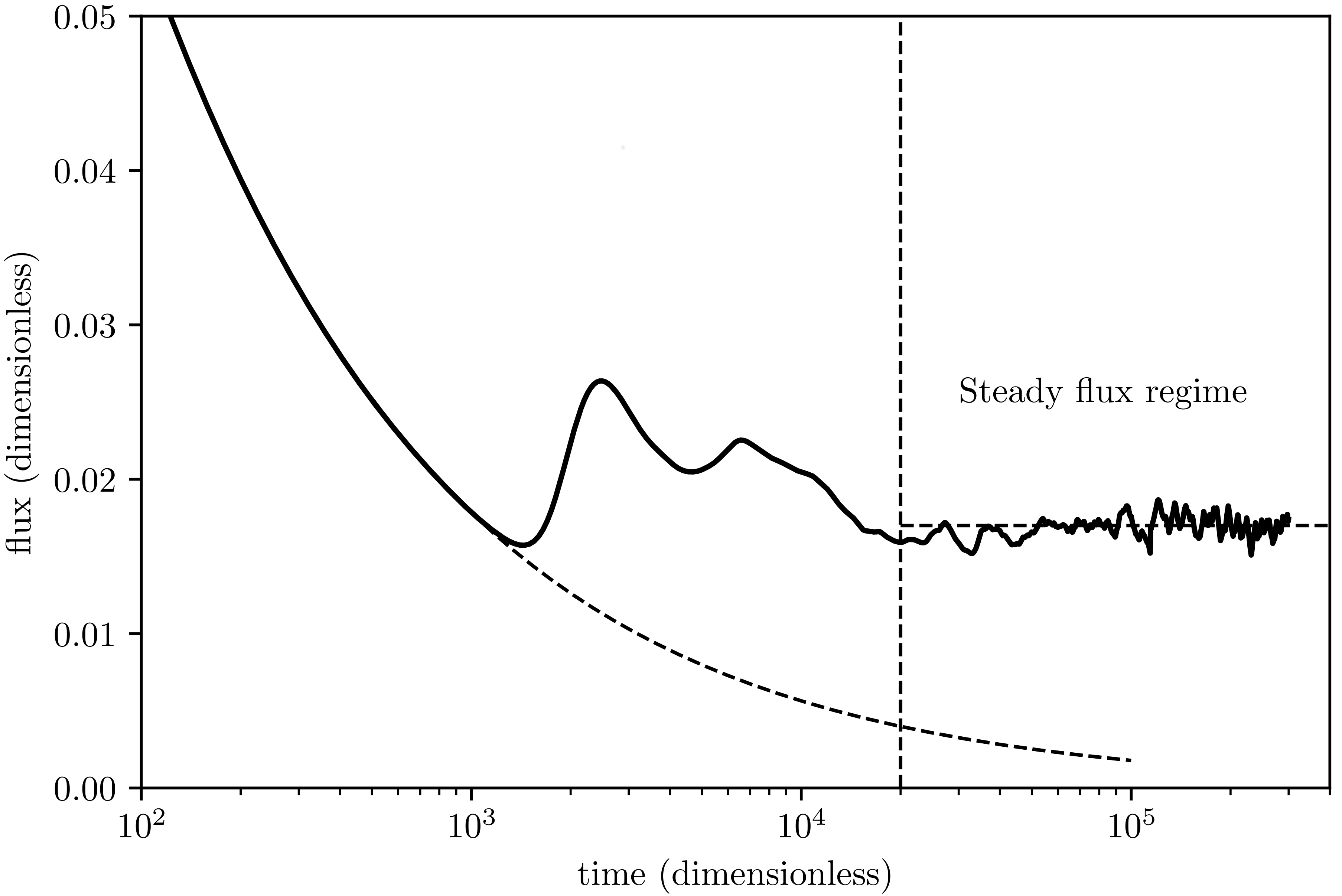
A large proportion of the theoretical studies concerning density-driven convective mixing in porous media that have appeared in the scientific literature have focussed on understanding the critical time for the onset of convection and the associated critical wavelength of fingers at the onset of convection in idealised homogeneous models (e.g., References [1,2,3,4,5,7,10,13,14]). One significant feature of density-driven convective mixing that has also received attention is the establishment of a steady long-term mass flux during the period after the fingers stabilise and before they reach the base of the aquifer, see Figure 1. Despite the complicated nature of the flow, only modest fluctuations in the rate of dissolution are observed in numerical simulations in this regime [9,10,15].
Solutal convection in realistic geological formations is typically a fine-scale process that occurs at a length scale several orders of magnitude below the typical computational resolution possible in field-scale simulations. For example, high-resolution simulations of convective mixing may use computational domains that are only a few metres in size, with spatial resolution at the cm or mm scale necessary in order to accurately model the complicated convective mixing process. The size and resolution of these models is in stark contrast to field-scale simulations of CO storage, where the computational expense commonly constrains the size of computational grid blocks to metres to tens of metres. The consequence of this disparity is to inhibit, and therefore delay, the onset of convective mixing in simulation studies with large grid blocks, which results in an underestimate of the total dissolved CO fraction [3].
Comparatively few studies have attempted to include the effect of enhanced dissolution due to density-driven convective mixing at the fine scale in large-scale simulation studies using coarse grid blocks. Initial attempts to include convective mixing in a coarse-scale model have included using a rudimentary sink term in the uppermost portion of the model to remove an amount of mobile CO equal to the theoretical estimate of the long-term average mass flux in order [16], or including the effect of convection through an upscaled representation of the mass transfer rate in a vertical equilibrium model [17,18]. Common to both of these studies are the assumptions that the onset time of the convective mixing process is small in comparison to the total simulation time, and that the dissolution rate can be approximated with the estimate of the steady flux. Using these models, it was found that including the enhanced dissolution due to sub-grid convective mixing reduced the up-dip migration of the gas-phase CO, and therefore the total time that the plume is mobile.
It is clear that the presence of a steady flux regime is likely to be significant in the development of an appropriate upscaling scheme for enhanced dissolution due to convective mixing, enabling this fine-scale process to be included in much larger grid blocks through some suitable mechanism. The availability of accurate theoretical estimates of the mass flux in the steady flux regime therefore underpins the establishment of upscaled models. For isotropic homogenous models, detailed numerical simulation studies have verified the functional form of the average dissolution rate in the steady flux regime, for both two-dimensional and three-dimensional models [9]. In practice, coarse simulation models are often constructed by upscaling fine-scale heterogeneous geological models to representative anisotropic homogeneous models with effective permeabilities. In this anisotropic case, a theoretical estimate of the average dissolution rate in the steady flux regime was shown to scale as for two-dimensional porous media only, where and are the effective vertical and horizontal permeabilities, respectively [15].
In this study, we consider the effect of anisotropy on the average long-term mass flux of CO in a three-dimensional saline aquifer, extending the work of Green and Ennis-King [15] for two dimensions. Numerical simulations of anisotropic porous media are used to verify that the scaling result for two-dimensional anisotropic porous media is also valid for three-dimensional porous media, despite the increased degrees of freedom present in three dimensions in comparison to two dimensions. Using high-resolution numerical simulations of heterogeneous three-dimensional porous media, we demonstrate that the average long-term mass flux is adequately represented by an equivalent anisotropic homogenous model, even though the vertical connectivity of these models is highly complex. Finally, we discuss how these results may be used as part of an upscaling method to incorporate the effects of subgrid-scale enhanced dissolution due to convective mixing in coarse-scale simulations of CO storage in saline aquifers.
2. Background Theory
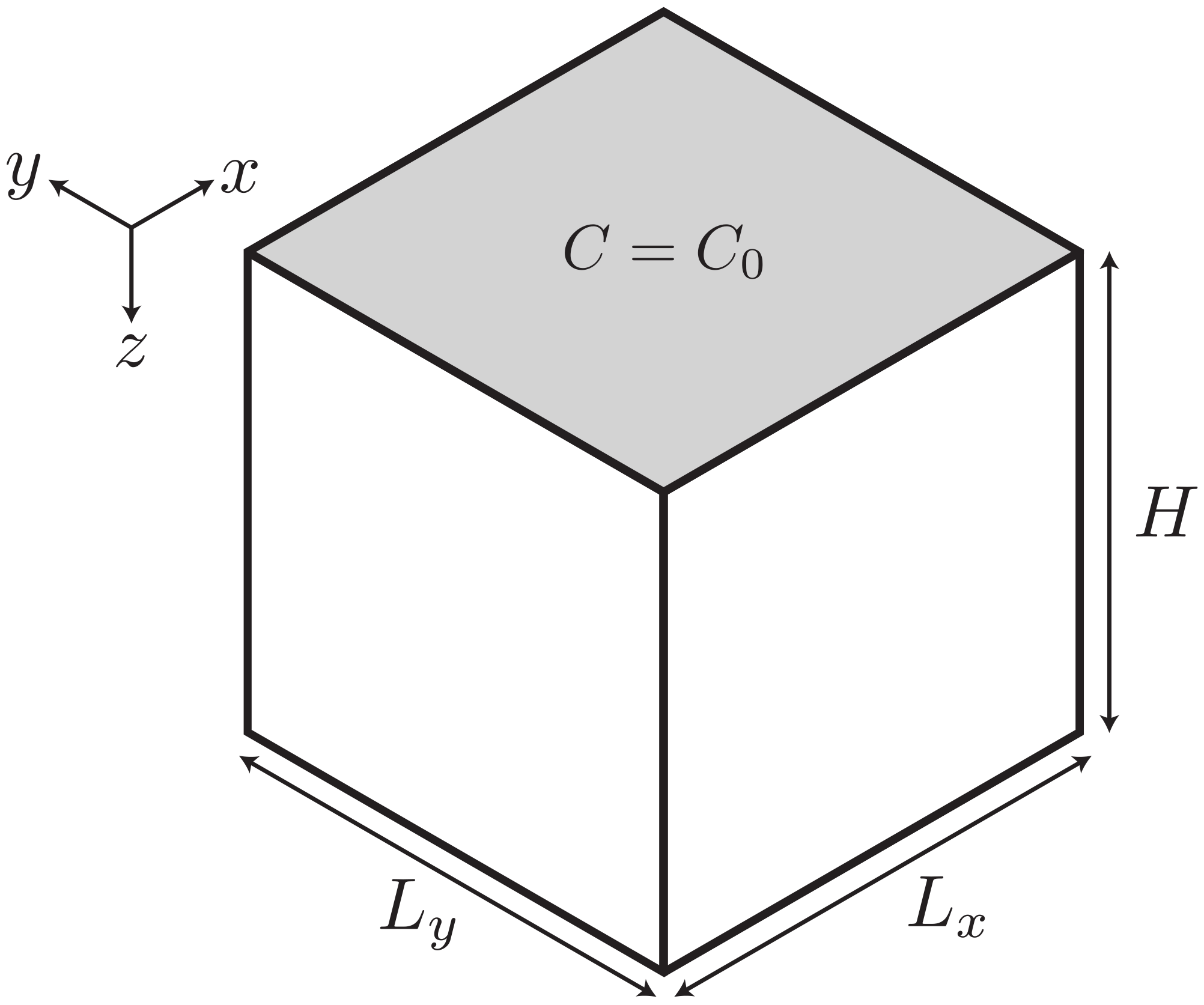
In this section, we present a brief overview of the theoretical background to the problem of density-driven convective mixing in porous media in three dimensions. For simplicity, we consider a cuboid model of height H and lengths and in the x and y directions, respectively, see Figure 2. The solute concentration, C, at the top surface () is fixed at equilibrium saturation . All parameters used in this analysis and their units are described in the table of nomenclature, Table 1.
Density-driven convective mixing of dissolved CO in porous media is a complex phenomenon governed by coupled partial differential equations, namely Darcy’s law and the convection-diffusion equation for transport of the dissolved solute. They are commonly expressed as
and
where is the Darcy velocity, k is permeability, is the dynamic viscosity, P is the pressure, is the fluid density, is the acceleration due to gravity, is the porosity of the porous medium, C is the solute concentration, t is time, and D is the effective diffusion coefficient (the product of diffusivity and tortuosity [2]). We also assume that the fluid is incompressible, whereby
Equations (1) and (2) are coupled by the change in fluid density as a result of the dissolved solute, which is typically provided using a relation of the form
where is the density of the unsaturated fluid, is the maximum solute concentration (i.e., the concentration at solute equilibrium), and is the maximum density increase with concentration. We restrict our study to the case where , i.e., the density of the fluid increases monotonically with increasing solute concentration, as is the case for CO dissolved in brine.
In order to simplify the problem, we invoke the Boussinesq approximation [19], in which case the dependence of on C is only retained in the buoyancy term in Equation (1). This simplifying assumption effectively linearises the dependence of density on concentration, which is appropriate for CO dissolved in brine due to the weak dependence of partial molar volume on concentration [2].
The governing equations are closed with appropriate boundary and initial conditions. Assuming that the porous media is an infinitely long, horizontal reservoir of fixed height H, the boundary conditions at the top () and bottom () surfaces are given by
respectively, where w is the vertical component of velocity. These boundary conditions correspond to a Dirichlet boundary at the upper surface (where the concentration is fixed at its equilibrium value), and a no-flux boundary at the lower surface. The presence of a fixed concentration boundary at the upper surface is supported by previous studies, where it was observed that the interface between the supercritical CO and brine remains sharp despite the presence of fingers of CO saturated brine sinking into the less dense unsaturated brine [3,20]. In reality, this assumption is a simplification of the true interface at the boundary layer, where two phases coexist. The initial conditions are
which correspond to no initial velocity and zero initial solute concentration in the reservoir (apart from the top boundary).
Significant insight into the problem can be obtained by non-dimensionalising the governing equations using suitable scales. As we are primarily interested in the steady flux regime during convective mixing in porous media, we only consider cases where the height of the model is much larger than the vertical distance over which convective instability forms [2]. Consequently, we scale lengths with the length over which convection and diffusion balance, so that horizontal lengths are scaled by and vertical lengths are scaled by [2], where and are the horizontal and vertical permeabilities, respectively (We only consider the case where permeability is the same in both horizontal directions for simplicity), and is the permeability anisotropy. Similarly, horizontal velocities are scaled by while vertical velocity is scaled by . Concentration C is scaled by , time is scaled by , and pressure is scaled by . The governing equations, boundary conditions and initial conditions become
where the superscript asterisk denotes a dimensionless variable, , and is the Rayleigh number, given by
This dimensionless number is a measure of the relative importance of density-driven convection to purely diffusive motion. When is sufficiently large, convection may occur. Using stability analysis, it has been shown that no convection is possible for [10]. For , convection is possible, with a minimum onset time depending on [10]. When , the earliest possible time for the onset of a convective instability is independent of [10].
We note that the Rayleigh number does not appear in the dimensionless governing equations, Equations (8) and (9). Rather, it appears only in the boundary condition at the base of the model, Equation (10), where the lower boundary is at a dimensionless depth . This is due to the length scale used in the parameterisation being the length at which diffusion and advection balance, rather than any geometrical length present in the model [21]. We choose this scaling as we are primarily interested in the steady flux regime, where the presence of a lower boundary does not influence the flux (a semi-infinite model) [21]. This is convenient for numerical models, as can be varied by simply changing the height of the model, with no scaling of the spatial resolution required as is varied.
Significant research effort has been undertaken to determine critical properties of density-driven convective mixing, such as the time for the onset of convection, and the wavelength of the initial perturbations for tractable cases of homogeneous porous media, both isotropic [3,4,5,10,20] and anisotropic [2,3,4,13]. A detailed review of these studies and the estimated values for critical parameters has been provided by Emamai-Meybodi et al. [14], to which the reader is referred for more information.
One of the most interesting features of solutal convection is the establishment of a steady flux regime, where the mass flux over the top boundary is relatively constant, with only small fluctuations about an average value observed despite the complex interaction between the fingers of saturated fluid and the unsaturated background fluid. High resolution numerical simulations have shown that the mass flux oscillates about a constant value in the long term, with temporal variations of the order of 15% (e.g., References [9,12,21]). This phenomena has also been observed experimentally in Hele-Shaw cells (e.g., References [8,22,23]).
The functional form of this long-term mass flux of CO per unit width in a two-dimensional model, , is given by [9]
where the constant is calculated from numerical results. Analogous results for three dimensions have demonstrated that the mass flux exhibits similar long-term behaviour as the two-dimensional case, albeit with a slightly increased prefactor [9,24].
Following Neufeld et al. [8], Green and Ennis-King [15] developed a simple theoretical scaling for the average dissolution flux in the steady flux regime in anisotropic two-dimensional porous media, which we provide here for completeness. The conceptual model is as follows: Downward moving plumes of CO-rich water are interspersed with upwelling plumes of fresh water. Once the upwelling plumes reach the top of the reservoir, they are forced laterally into a mixing region [8]. The lateral flow in the mixing region acts to stabilise the diffusive boundary layer, which has thickness , where l is the width of the upwelling plume, and u is the lateral fluid velocity in the mixing region.
When the porous media is isotropic, the lateral fluid velocity is equal to the vertical velocity of fluid in the upwelling plume [8]. If the porous media is anisotropic, however, the principle of conservation of mass dictates that the ratio of the thickness of the horizontal mixing region to the width of the upwelling plume is equal to . It then follows that ratio of the vertical fluid velocity in the upwelling plume to the lateral fluid velocity in the mixing region must scale as . The width of the upwelling plume is inversely proportional to to first order [2], while vertical velocity in the upwelling plumes scales as . The total flux into the porous media across the upper boundary, which is equal to the flux across the boundary layer [8], therefore scales as in an anisotropic porous media.
This result suggests that it is the geometric mean of the vertical and horizontal permeabilities that should be used in the estimate of the mass flux in the steady flux regime [15], in which case the average long-term mass flux for a two-dimensional anisotropic porous media is
i.e., Equation (14) scaled by and replacing k with . This functional relationship has been verified through two-dimensional numerical simulations of anisotropic homogeneous porous media [15,25].
Green and Ennis-King [26] demonstrated through numerical simulations that the average mass flux in the steady flux regime during solutal convection in a two-dimensional heterogeneous porous medium was well represented by an anisotropic homogeneous porous medium with equivalent permeabilities in the vertical and horizontal directions. Several subsequent studies have also observed that the steady flux rate is dependent on the average properties of the porous medium, suggesting that heterogeneous porous media may be suitably modelled using anisotropic homogeneous porous media [15,27,28,29,30].
3. Numerical Method
To date, the scaling relationship for the average mass flux in the steady flow regime, Equation (15), has not been demonstrated for anisotropic and heterogeneous three-dimensional models. It is important to verify (or otherwise disprove) the theoretical scaling presented by Green and Ennis-King [15] for two-dimensional convective mixing in the three-dimensional case. To that end, we have undertaken a series of high-resolution simulations of density-driven convective mixing in both anisotropic and heterogeneous porous media.
High-resolution numerical simulations were performed using Numbat [31] (https://github.com/cpgr/numbat), an open-source application developed by the authors using the Multiphysics Object-Oriented Simulation Environment (MOOSE) software framework [32] (http://www.mooseframework.org). Numbat solves either the dimensional (Equations (1)–(4)) or dimensionless (Equations (8) and (9)) form of the governing equations using the finite element method, and leverages powerful features of the open-source MOOSE framework, such as adaptive mesh refinement, automatic parallelism, and both continuous and discontinuous Galerkin methods to enable massively parallel simulations of density-driven convective mixing in porous media. In this study, numerical simulations using both the dimensional and dimensionless forms are used to determine the average mass flux in the steady flux regime in three-dimensional models. Fully unstructured computational meshes were used in this study, with a fine discretisation near the top boundary to adequately resolve the initial fingers, and a coarser discretisation towards the base of the model where fingers are large. At least several million elements are used in each of the three-dimensional meshes. Due to the large number of elements, each simulation was run using between 100 and 1000 cores on a large computational cluster.
The dimensionless form of the governing equations, Equation (8) and (9), are solved using a stream function formulation [21,33]. For details, see Appendix A.
Numbat has been benchmarked against previously published results in two and three dimensions, detailed by Pruess and Zhang [34] and Pau et al. [9]. Qualitatively, the results obtained using Numbat are consistent with those studies. The steady flux values in these cases are similar to those reported by Pruess and Zhang [34] and Pau et al. [9]. Small differences in the onset time are observed, but these are likely the result of the difference in the random noise used to seed the instability. Full details are provided in the Numbat user manual [31].
It is well known that the onset time of convection is sensitive to the initial disturbance used to seed the gravitational instability that is the driver of convective mixing [14], whereas the steady mass flux is insensitive to the choice of initial disturbance [14]. In this study, the gravitational instability is seeded by perturbing the model in a controlled manner. For dimensional simulations, a random noise of amplitude is added to the initial porosity field [26], while for the dimensionless simulations, a reproducible random noise is added to the initial diffusive concentration field [21].
No-flow boundaries are imposed on the upper and lower faces of the model, while lateral periodicity is imposed through periodic boundary conditions. The upper boundary is fixed at a given concentration, either for the dimensionless model, or for the dimensional case, for some equilibrium concentration .
Anisotropy is imposed through varying the anisotropy ratio in the dimensionless model. The computational models used in these anisotropic simulations have a dimensionless length of 3000 in each of the horizontal directions, and a dimensionless length of 5000 in the vertical direction. The height of the model corresponds to a Rayleigh number of [10]. The horizontal lengths are chosen so that a sufficiently large number of fingers are present in the model. The wavelength of the fingers at the onset of convection has the functional form , where the parameter has been estimated by various authors as [2], [4], or [13]. These estimates suggest that there will be at least one hundred fingers in the model at the onset of convection for the smallest value of anisotropy ratio, and up to several hundred for the isotropic case.
Two models of reservoir heterogeneity are considered in this study. Following the use of horizontal flow barriers as a simplified proxy for realistic heterogeneity (such as shale filled reservoirs) in two-dimensional studies of convective mixing [15,26,27,28,30], we extend this idea to three dimensions using flat elliptical disks of various aspect ratios to represent flow barriers. The major and minor axes of the elliptical disks are drawn from Gaussian distributions and , respectively, where refers to a Gaussian distribution with mean and standard deviation . Barrier dimensions were chosen so as to be larger than the typical finger length in the upper region of the computational mesh to provide a significant impediment to downwards flow. The distribution of barriers used in this study is depicted in Figure 3. The mesh was suitably refined in the vicinity of the barriers to accurately capture their geometry. The distribution of barriers shown in Figure 3 results in a permeability anisotropy of . As for the anisotropic models, the dimensionless forms of the governing equations are solved in this case. The horizontal dimensions again have a dimensionless length of 3000, while the model has a dimensionless height of 5000.
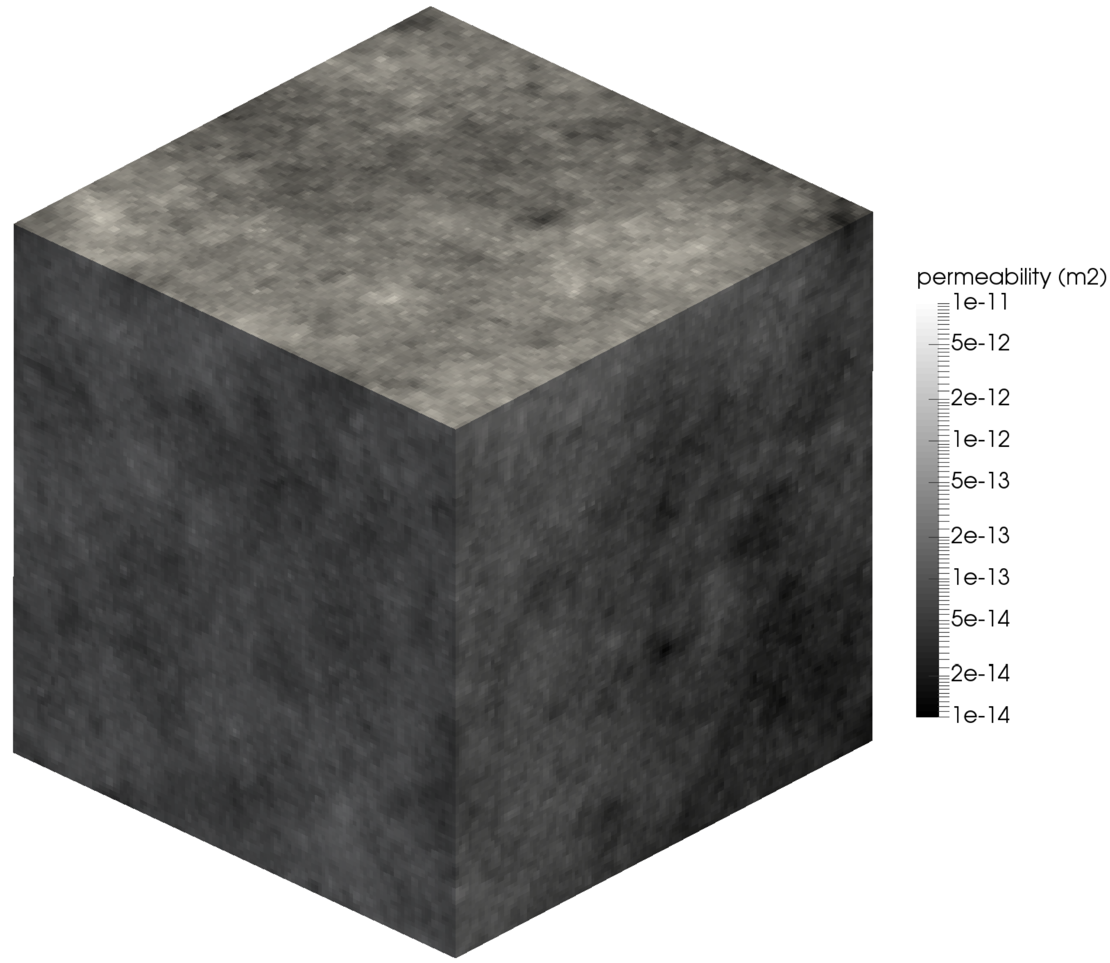
The second model of heterogeneity uses fractional Lévy motion (fLm) to generate a spatially-varying permeability field, as non-Gaussian structure has been observed in sedimentary formations [35,36,37]. A model with fLm structure was generated using a midpoint displacement algorithm with successive random additions [38] drawn from a Lévy distribution with width parameter and Hurst parameter [39]. A heterogeneous permeability field was then constructed as , where m is a mean permeability (approximately 400 mD), and is a random number sampled from the Lévy distribution with width parameter and Hurst parameter H. This results in a heterogeneous model with permeability varying over three orders of magnitude, see Figure 4. Within each cell, the vertical permeability was scaled so that the overall permeability anisotropy was . All other reservoir properties are representative of a low salinity aquifer at a depth of approximately 1 km, and are given in Table 2. The dimensions of the model are 10 m in all directions.
In contrast to the two-dimensional case, where multiple statistical realisations of heterogeneity are used to investigate their effect on solutal convection [15,26], the computational expense of three-dimensional simulations precludes a probabilistic study. As a result, only two statistical realisations of each permeability heterogeneity are considered.
4. Results
4.1. Anisotropic Porous Media
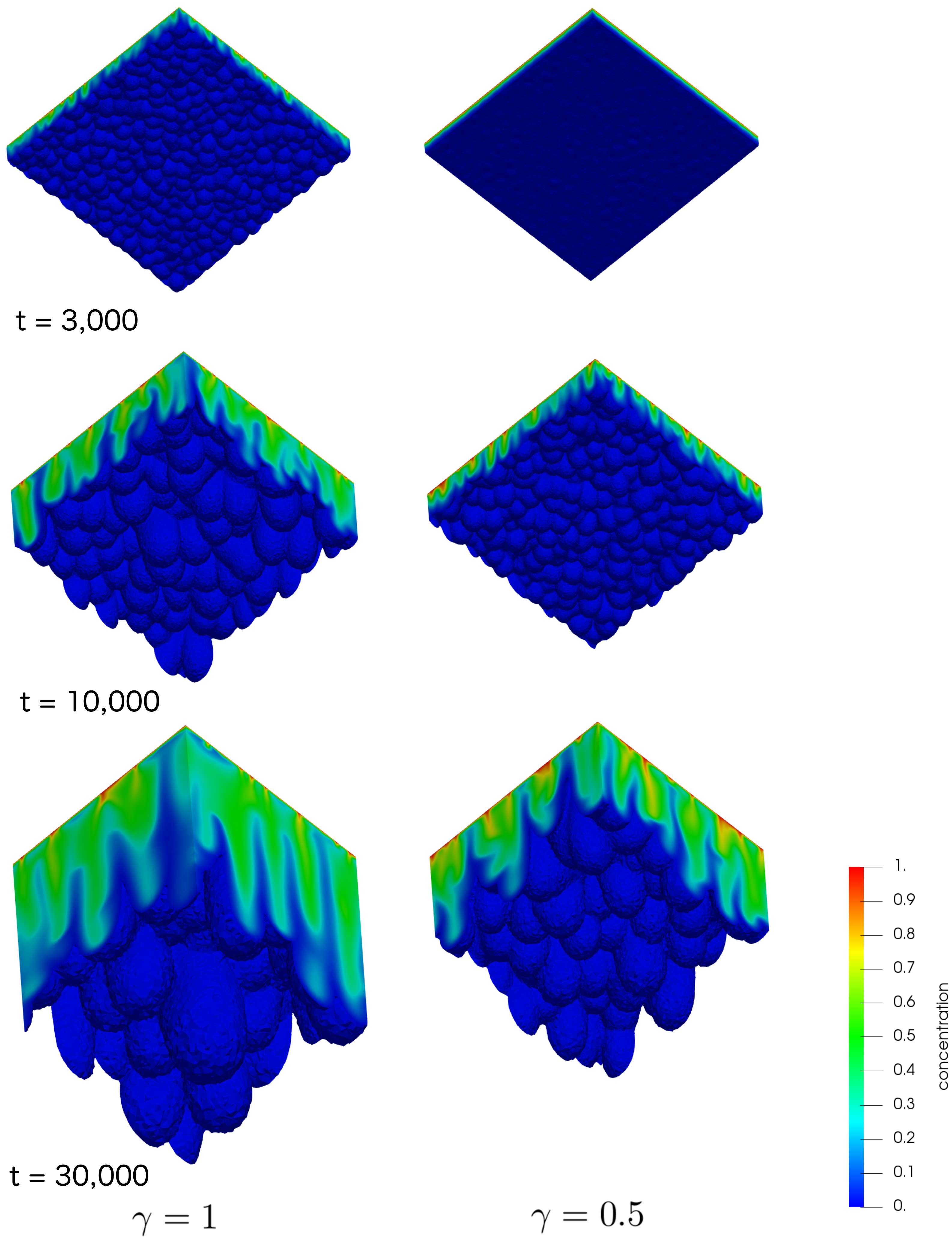
Numerical simulations of three-dimensional convective mixing in homogeneous but anisotropic porous media were performed for permeability anisotropies , , and using the dimensionless form of the governing equations. Figure 5 presents a comparison of an isotropic model () with an anisotropic model (). As this comparison shows, we observe that anisotropy delays the onset of convection in comparison with the isotropic case, as evidenced by the slower formation of downwelling fingers in the anisotropic case, see Figure 5. This is in line with previous findings for convective mixing in two-dimensional porous media [2,15].
Figure 5 also demonstrates that the lateral dimension of the fingers at the onset of convection is larger for in comparison for (remembering that lateral dimensions scale as ). This can be observed by comparing the initial finger pattern at for the isotropic case with the finger pattern for the anisotropic case at a similar finger depth (at a later time t = 10,000 due to the delayed onset of convection in the anisotropic case in comparison to the isotropic case), where fewer fingers can be seen.
The effect of permeability anisotropy can be quantified by comparing the temporal evolution of the flux across the top boundary for the isotropic and anisotropic cases, which is calculated as
where and are the lengths of the computational model in the x and y directions, respectively, see Figure 2.
As Figure 6 demonstrates, decreasing delays the onset of convection, which results in a smaller average flux in the steady flux regime.
For the isotropic case (), the average flux in the steady flux regime was calculated as , slightly larger than the accepted value for two-dimensional models (). This finding is commensurate with the previous observations of steady flux in isotropic homogeneous porous media in three dimensions [9]. Likewise, we observe smaller oscillations about this average flux in three dimensions, which is likely the result of the increased number of fingers in the three-dimensional model.
4.2. Heterogeneous Porous Media
One of the important results presented in earlier studies of density-driven convective mixing in two-dimensional heterogeneous porous media is that the steady flux in a heterogeneous model is well-approximated by the flux in an equivalent anisotropic homogeneous model [15,26], which implies that a heterogeneous model of the porous media can be replaced with a simpler anisotropic homogeneous model. We now present numerical results to verify this in three dimensions using the two examples of permeability heterogeneity discussed earlier.
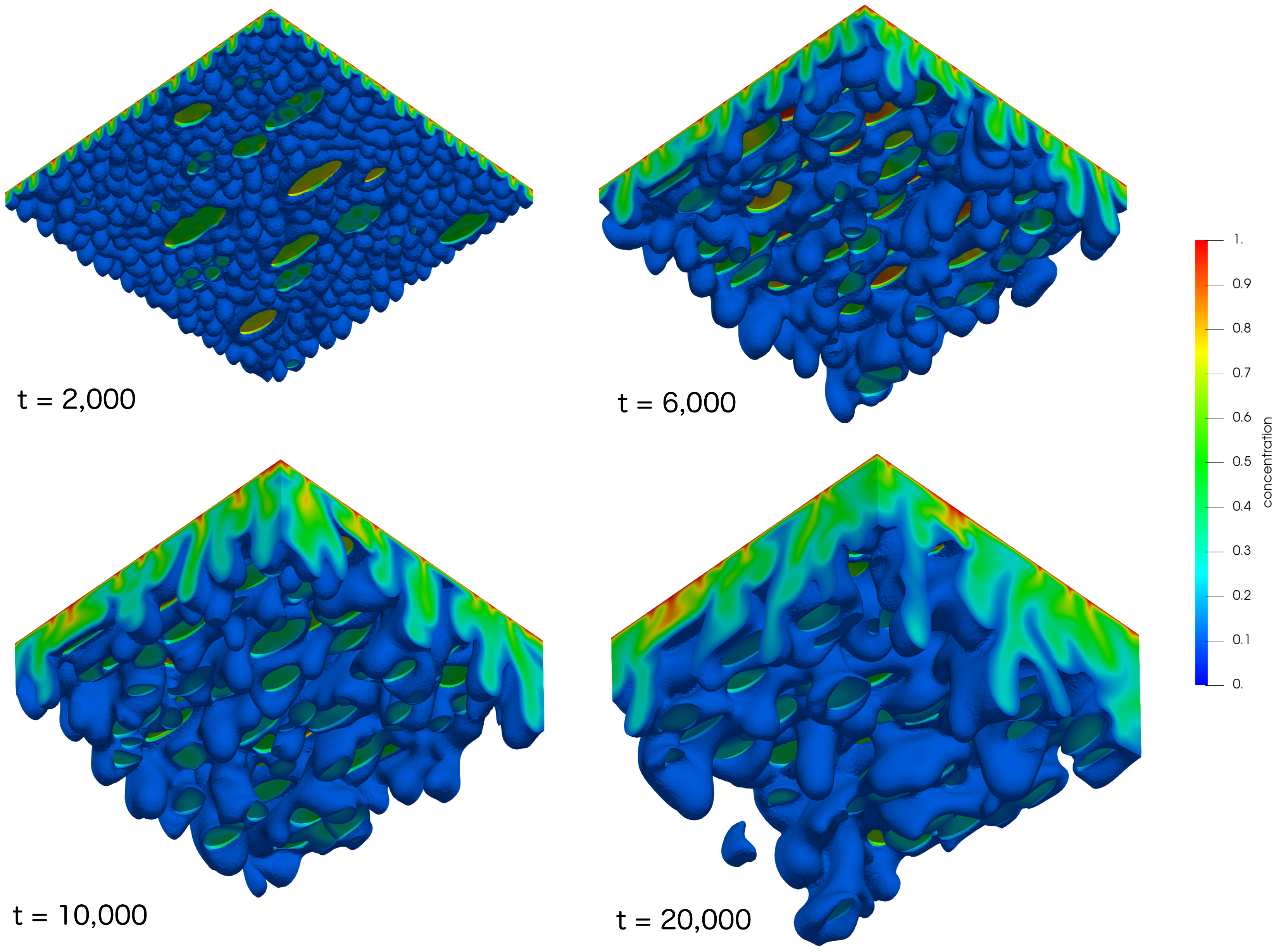
The temporal evolution of the concentration in the heterogeneous model with elliptical flow barriers is presented in Figure 7. Initially, small fingers form around the barriers, with an increased concentration observed on the upper surface of the barriers. As time increases, the downwelling fingers merge to form larger fingers which totally encapsulate the barriers. These then flow downwards until they reach the next barrier, and the process is repeated.
It is clearly evident from Figure 7 that the barriers have a significant effect on the dynamics of the fingers, impeding their downward motion and resulting in extremely complex finger patterns. Nevertheless, the average flux in the steady flux regime for this complex model is well approximated by the average flux in an equivalent anisotropic homogeneous model, see Figure 8. In contrast, we observe that the onset time for convection is much earlier for the heterogeneous barrier model in comparison to the equivalent anisotropic model, providing more evidence that the onset time is sensitive to the local permeability whereas the steady flux is governed by the global average permeability [15,26]. In fact, comparing the onset time for the heterogeneous model in Figure 8 with the onset time for the isotropic porous medium in Figure 6, we find that they are nearly identical. As both models use an equivalent formulation, with the permeability in the background of the heterogeneous model equivalent to the isotropic case, this result provides further evidence for the hypothesis that it is the local permeability that influences the onset of convective mixing in heterogeneous porous media [15,26].
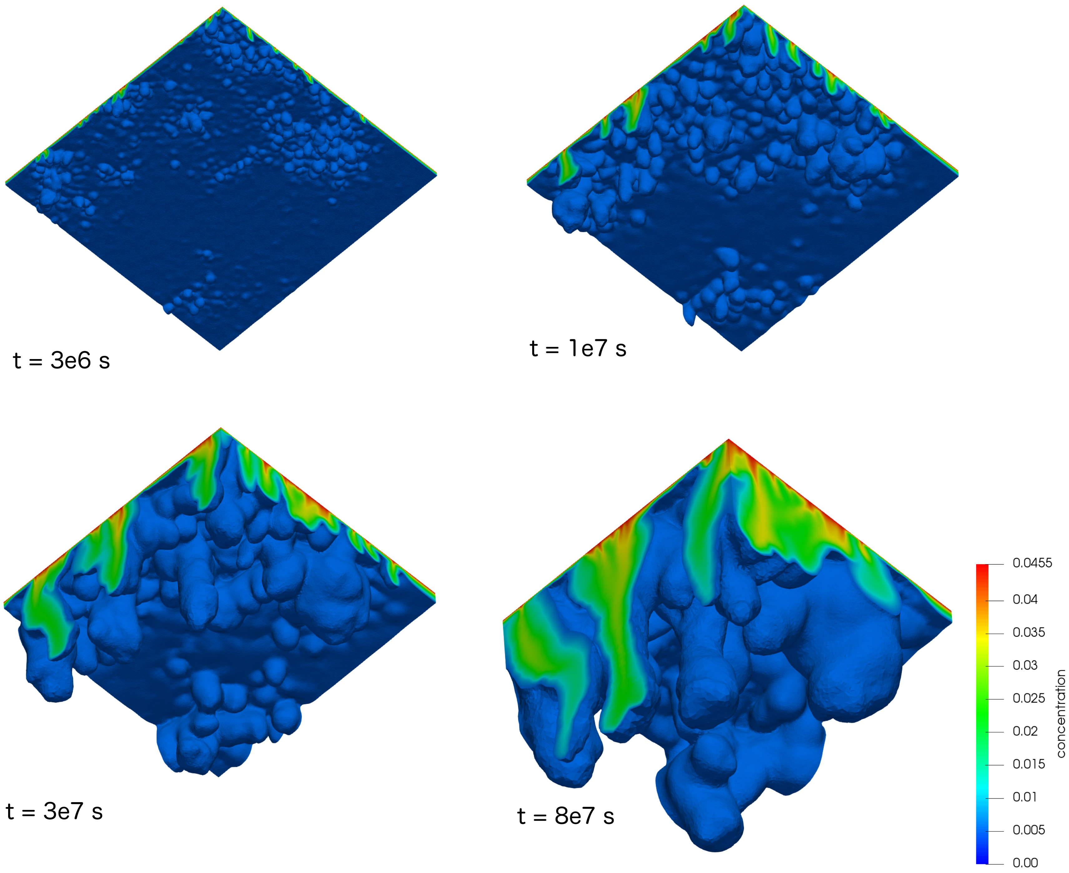
In the second case of heterogeneity, the dimensional form of the governing equations are solved for the case of permeability heterogeneity constructed using a fractional Lévy motion model. In this case, convective fingers are observed to form in the higher permeability regions initially, with no fingers observed in the regions of lower permeability, see Figure 9. At this early time, we conclude that it is the local permeability that controls the onset and growth of fingers. As time increases, these initially small fingers merge to form larger fingers, as usual. Eventually, the fingers become large enough, after which it is the average permeability that governs their motion, and we observe that fingers are now present throughout the porous media, even in those regions where the permeability is low.
This is clearly illustrated in the temporal progression depicted in Figure 10, where the contours of concentration are provided along a horizontal slice a distance of 0.5 m from the upper surface of the model. After s, fingers can be observed in the regions of higher permeability, with no fingers present in the regions of lower permeability. As time increases, we can observe that the fingers join into laterally extensive plumes that begin to include the lower permeability region.
The flux across the top boundary for the fractional Lévy motion model of permeability heterogeneity is presented in Figure 11, alongside the flux in an anisotropic homogeneous model with equivalent effective permeabilities in the vertical and horizontal directions. Again, the steady flux in the heterogeneous model is well approximated by the flux in the equivalent anisotropic model, providing further evidence that the complex motion in the steady flux regime of density-driven convective mixing in heterogeneous porous media can be adequately modelled using simpler anisotropic homogeneous models with effective permeabilities.
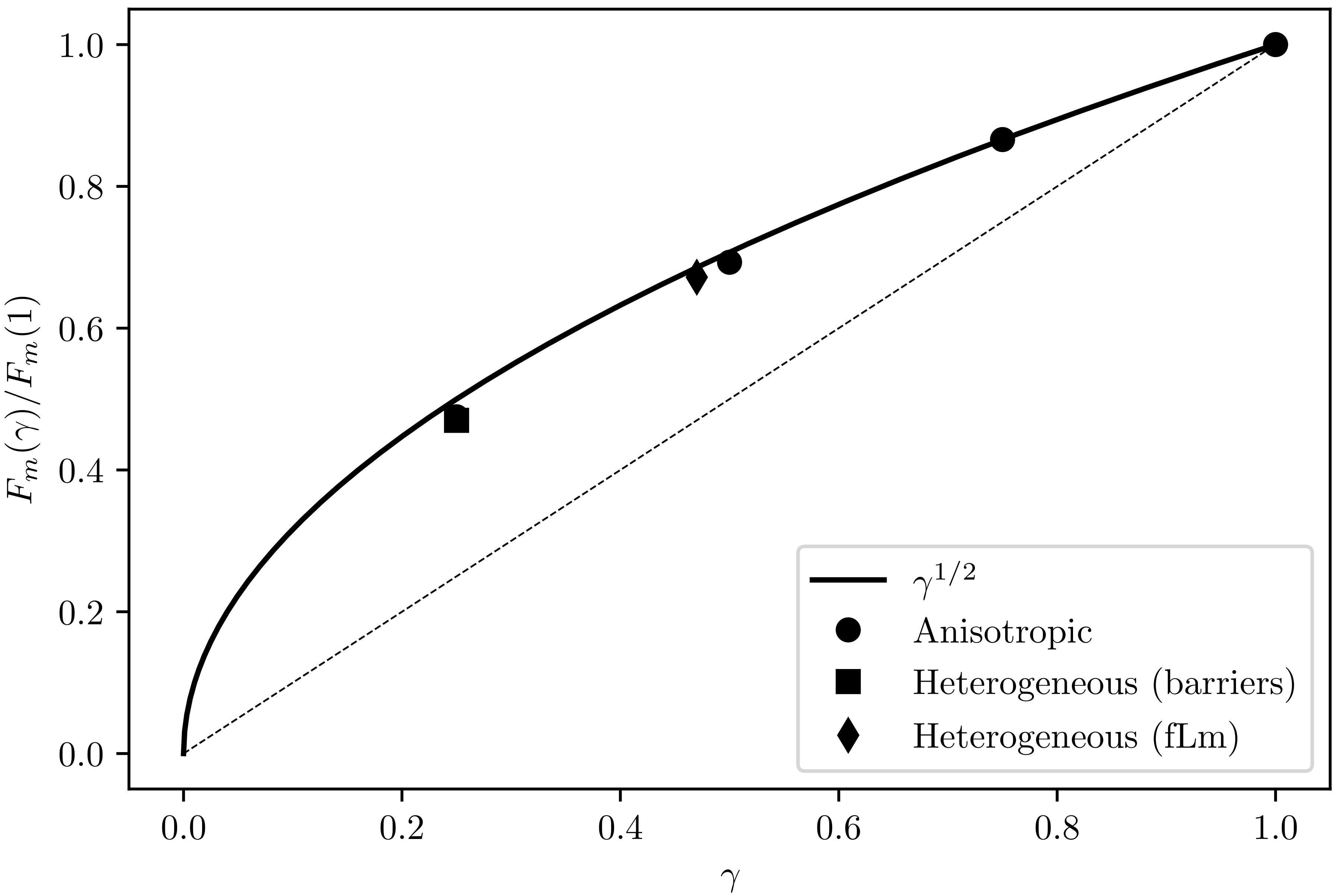
The calculated steady fluxes for all three-dimensional cases considered are summarised in Figure 12, where the average flux is calculated from the numerical results in the steady-flux regime. These results clearly demonstrate that the theoretical scaling for the steady flux in anisotropic porous media presented by Green and Ennis-King [15] for two-dimensional porous media is also applicable to density-driven convective mixing in three-dimensional porous media, but with the prefactor increased to :
This is despite the increased complexity observed in three-dimensional porous media in contrast to two-dimensional porous media due to the added degrees of freedom. Importantly, these results demonstrate that this scaling may also be appropriate in heterogeneous three-dimensional porous media, suggesting that the long-term dissolution in a heterogeneous model may be well approximated with a simple anisotropic model.
5. Discussion
High-resolution numerical simulations of density-driven convective mixing in three-dimensional porous media have been undertaken to examine the applicability of the theoretical scaling for the steady flux in two-dimensional models developed by Green and Ennis-King [15] to three-dimensional models. In so doing, it was demonstrated that the average mass flux in the steady flux regime also scales as in three dimensional anisotropic porous media.
Two models of permeability heterogeneity were considered, and in each case, it was demonstrated that the magnitude of the average flux in the steady flux regime for these models of permeability heterogeneity were well represented by anisotropic homogeneous porous models with effective permeabilities that provide an equivalent Darcy flux. This finding extends the earlier findings for two-dimensional heterogeneous porous media [15,26] to the more realistic case of three-dimensional models. Qualitatively similar behaviour between heterogeneous and homogeneous three-dimensional models were obtained by Soltanian et al. [29] for different models of heterogeneity when comparing the dynamics of convection using a different measure of convection to the steady flux considered here.
In both cases of heterogeneity studied here, we observed that the onset time of convection was shorter in the heterogeneous model in comparison to the equivalent anisotropic model. This lends further support to the hypothesis that local regions of comparatively high permeability can influence the critical onset time and wavelength of the fingers in heterogeneous media [15]. These regions of high local permeability are not present in the anisotropic model, having been averaged out through upscaling to effective permeabilities. As a result, the onset time is delayed in anisotropic models in comparison to heterogeneous models. This is in contrast to the steady flux, which appears to be insensitive to local permeability and is instead governed by the large-scale effective permeability [15,26].
The observation that convection occurs much sooner in heterogeneous models in comparison to an equivalent anisotropic homogeneous model while still exhibiting similar average flux in the steady flux regime over the long term suggests that it may be possible to incorporate the enhanced dissolution due to convection at the fine-scale in coarse-scale simulations, by assuming that convection begins immediately and that the rate of mass flux into the liquid phase is constant while a gas phase remains present. This lends support to initial attempts to include enhanced dissolution due to convection at the sub-grid scale using these simplifying assumptions [16,17,18].
Due to the fundamental importance of convective mixing on the rate of dissolution and hence the total amount of CO that is immobilised in the denser liquid phase, upscaled models that implement this accelerated dissolution are necessary for reliable numerical predictions of the long-term fate of CO storage in saline aquifers. These upscaled models must be informed by theoretical estimates of the dissolution events, such as average dissolution in the steady flux regime [9,15,21]. As previously discussed, results such as those presented here, as well as earlier studies [15,26,27,29], suggest that it may be possible to approximate the steady flux regime in heterogenous porous media using an upscaled model with effective parameters. Additionally, if the onset time for convection is small in comparison to the total simulation time, then the dissolution flux may, to first order, be approximated by the steady flux for all time (as implemented in previous attempts to incorporate enhanced dissolution due to convection in large-scale models as discussed above [16,17,18]). This implies that it may be possible to adequately represent a heterogeneous model with an anisotropic model with equivalent effective permeabilities, even though the onset time in the heterogeneous model is likely to be earlier than in the anisotropic model. This follows from the observation that if the rate of dissolution in both heterogeneous and anisotropic models is similar, then the relative difference between the total dissolved solute due to the difference in onset time in both cases becomes smaller as time increases. If the total simulation time greatly exceeds the onset time, then the difference due to the delayed onset time in the anisotropic model is likely to be small in comparison to the total dissolved amount.
The results presented in this study have been obtained using an idealised representation of the physics involved. Only a single fluid phase has been considered, with an unlimited supply of saturated fluid provided using a constant concentration boundary condition at the top surface. This is a commonly used simplification of the more realistic two-phase boundary that would exist at the interface of the saturated and unsaturated fluids. The presence of a capillary transition zone has also been ignored, as has the possibility of geochemical reactions. Different realisations of permeability heterogeneity may result in cases where the steady flux regime is not adequately represented using an equivalent anisotropic model. A detailed review of the impact that these complicating factors may have on the convective mixing process can be found in Emami-Meybodi et al. [14], to which the reader is referred for further details.
Author Contributions
Conceptualization, J.E.-K.; Methodology, C.P.G.; Software, C.P.G.; Validation, C.P.G.; Formal Analysis, C.P.G. and J.E.-K.; Investigation, C.P.G. and J.E.-K.; Resources, C.P.G.; Data Curation, C.P.G.; Writing—Original Draft Preparation, C.P.G.; Writing—Review & Editing, C.P.G. and J.E.-K.; Visualization, C.P.G.; Supervision, J.E.-K.; Project Administration, J.E.-K.; Funding Acquisition, J.E.-K.
Funding
The authors wish to acknowledge financial assistance provided through the Australian National Low Emissions Coal Research and Development (ANLEC R&D). ANLEC R&D is supported by Australian Coal Association Low Emissions Technology Limited and the Australian Government through the Clean Energy Initiative.
Conflicts of Interest
The authors declare no conflict of interest.
Appendix A. Streamfunction Solution to Non-Dimensional Governing Equations
The details of the solution method for the dimensionless form of the governing equations is presented here. For brevity, notation is simplified by removing any asterisks used to denote a dimensionless quantity.
Appendix A.1. Two-Dimensional Formulation
Following Slim [21], Equations (8) and (9) are solved in two dimensions by introducing the streamfunction
Immediately, the continuity equation, Equation (3), is satisfied.
The pressure P is removed from Darcy’s equation, Equation (8), by taking the curl of both sides and noting that for any scalar P, and Darcy’s equation reduces to
Substituting the streamfunction into the convection-diffusion equation, Equation (8), we obtain
Similarly, the boundary conditions become
while the initial condition remains unchanged.
Appendix A.2. Three-Dimensional Formulation
To solve these governing equations in three dimensions, a different approach must be used as the streamfunction is not defined. Instead, we define a vector potential following Hewitt et al. [33] such that
It is important to note that the vector potential is only known up to the addition of the gradient of a scalar
as for any scalar . This uncertainty is referred to as gauge freedom [33] Taking the curl of Equation (8) and introducing , we have
where we have again used the fact that to eliminate pressure from the governing equations.
If we choose to specify the gauge condition, this simplifies to
The condition is satisfied throughout the domain if [40]
The governing equations are then
where the continuity is satisfied automatically, because for any .
Finally, it is straightforward to show that in order to satisfy and , which means that the vector potential has only x and y components,
and therefore the fluid velocity is
It is simple to show that and at are only satisfied if in the entire domain. In this case, the governing equations reduce to the two-dimensional formulation, as expected.
References
- Lindeberg, E.; Wessel-Berg, D. Vertical convection in an aquifer column under a gas cap of CO2. Energy Convers. Manag. 1997, 38, S229–S234. [Google Scholar] [CrossRef]
- Ennis-King, J.P.; Preston, I.; Paterson, L. Onset of convection in anisotropic porous media subject to a rapid change in boundary conditions. Phys. Fluids 2005, 17, 084107. [Google Scholar] [CrossRef]
- Ennis-King, J.P.; Paterson, L. Role of convective mixing in the long-term storage of carbon dioxide in deep saline formations. SPE J. 2005, 10, 349–356. [Google Scholar] [CrossRef]
- Xu, X.F.; Chen, S.Y.; Zhang, D.X. Convective stability analysis of the long-term storage of carbon dioxide in deep saline aquifers. Adv. Water Resour. 2006, 29, 397–407. [Google Scholar] [CrossRef]
- Riaz, A.; Hesse, M.; Tchelepi, H.A.; Orr, F.M. Onset of convection in a gravitationally unstable diffusive boundary layer in porous media. J. Fluid Mech. 2006, 548, 87–111. [Google Scholar] [CrossRef]
- Hassanzadeh, H.; Pooladi-Darvish, M.; Keith, D.W. Scaling behavior of convective mixing, with application to geological storage of CO2. AIChE J. 2007, 53, 1121–1131. [Google Scholar] [CrossRef]
- Rees, D.A.S.; Selim, A.; Ennis-King, J.P. The instability of unsteady boundary layers in porous media. In Emerging Topics in Heat and Mass Transfer in Porous Media; Vadasz, P., Ed.; Springer: Amsterdam, The Netherlands, 2008; Chapter 4. [Google Scholar]
- Neufeld, J.A.; Hesse, M.A.; Riaz, A.; Hallworth, M.A.; Tchelepi, H.A.; Huppert, H.E. Convective dissolution of carbon dioxide in saline aquifers. Geophys. Res. Lett. 2010, 37, L22404. [Google Scholar] [CrossRef]
- Pau, G.S.; Bell, J.B.; Pruess, K.; Almgren, A.S.; Lijewski, M.J.; Zhang, K. High-resolution simulation and characterization of density-driven flow in CO2 storage in saline aquifers. Adv. Water Res. 2010, 33, 443–455. [Google Scholar] [CrossRef]
- Slim, A.C.; Ramakrishnan, T.S. Onset and cessation of time-dependent, dissolution-driven convection in porous media. Phys. Fluids 2010, 22, 124103. [Google Scholar] [CrossRef]
- Kneafsey, T.J.; Pruess, K. Laboratory flow experiments for visualizing carbon dioxide-induced, density-driven brine convection. Transp. Porous Med. 2010, 82, 123–139. [Google Scholar] [CrossRef]
- Hidalgo, J.J.; Fe, J.; Cueto-Felgueroso, L.; Juanes, R. Scaling of convective mixing in porous media. Phys. Rev. Lett. 2012, 109, 264503. [Google Scholar] [CrossRef] [PubMed]
- Cheng, P.; Besehorn, M.; Firoozabadi, A. Effect of permeability anisotropy on buoyancy-driven flow for CO2 sequestration in saline aquifers. Water Resour. Res. 2012, 48, W09539. [Google Scholar] [CrossRef]
- Emami-Meybodi, H.; Hassanzadeh, H.; Green, C.P.; Ennis-King, J. Convective dissolution of CO2 in saline aquifers: Progress in modeling and experiments. Int. J. Greenh. Gas Control 2015, 40, 238–266. [Google Scholar] [CrossRef]
- Green, C.P.; Ennis-King, J. Steady dissolution rate due to convective mixing in anisotropic porous media. Adv. Water Res. 2014, 73, 65–73. [Google Scholar] [CrossRef]
- Pruess, K.; Nordbotten, J.M. Numerical Simulation Studies of the Long-term Evolution of a CO2 Plume in a Saline Aquifer with a Sloping Caprock. Transp. Porous Med. 2011, 90, 135–151. [Google Scholar] [CrossRef] [Green Version]
- Gasda, S.E.; Nordbotten, J.M.; Celia, M.A. Vertically averaged approaches for CO2 migration with solubility trapping. Water Resour. Res. 2011, 47, W05528. [Google Scholar] [CrossRef]
- Gasda, S.E.; Nordbotten, J.M.; Celia, M.A. Application of simplified models to CO2 migration and immobilization in large-scale geological systems. Int. J. Greenh. Gas Control 2012, 9, 72–84. [Google Scholar] [CrossRef]
- Bear, J. Dynamics of Fluids in Porous Media; Dover Publications: New York, NY, USA, 1972. [Google Scholar]
- Lindeberg, E.; Bergmo, P.E.S. The long-term fate of CO2 injected into an aquifer. In Proceedings of the Sixth International Conference on Greenhouse Gas Control Technologies, Kyoto, Japan, 1–4 October 2002; Volume 1, pp. 489–494. [Google Scholar]
- Slim, A. Solutal-convection regimes in a two-dimensional porous medium. J. Fluid Mech. 2014, 741, 461–491. [Google Scholar] [CrossRef]
- Backhaus, S.; Turitsyn, K.; Ecke, R. Convective instability and mass transport of diffusion layers in a Hele-Shaw geometry. Phys. Rev. Lett. 2011, 106, 104501. [Google Scholar] [CrossRef] [PubMed]
- Slim, A.C.; Bandi, M.; Miller, J.C.; Mahadevan, L. Dissolution-driven convection in a Hele–Shaw cell. Phys. Fluids 2013, 25, 024101. [Google Scholar] [CrossRef]
- Fu, X.; Cueto-Felgueroso, L.; Juanes, R. Pattern formation and coarsening dynamics in three-dimensional convective mixing in porous media. Phil. Trans. R. Soc. A 2013, 371, 20120355. [Google Scholar] [CrossRef] [PubMed]
- De Paoli, M.; Zonta, F.; Soldati, A. Dissolution in anisotropic porous media: Modelling convection regimes from onset to shutdown. Phys. Fluids 2017, 29, 026601. [Google Scholar] [CrossRef]
- Green, C.P.; Ennis-King, J.P. Effect of Vertical Heterogeneity on Long-Term Migration of CO2 in Saline Formations. Transp. Porous Med. 2010, 82, 31–47. [Google Scholar] [CrossRef]
- Lindeberg, E.; Wessel-Berg, D. Upscaling studies of diffusion induced convection in homogeneous and heterogeneous aquifers. Energy Procedia 2011, 4, 3927–3934. [Google Scholar] [CrossRef]
- Elenius, M.T.; Gasda, S.E. Convective mixing in formations with horizontal barriers. Adv. Water Res. 2013, 62, 499–510. [Google Scholar] [CrossRef]
- Soltanian, M.R.; Amooie, M.A.; Gershenzon, N.; Dai, Z.; Ritzi, R.; Xiong, F.; Cole, D.R.; Moortgat, J. Dissolution Trapping of Carbon Dioxide in Heterogeneous Aquifers. Environ. Sci. Technol. 2017, 51, 7732–7741. [Google Scholar] [CrossRef] [PubMed]
- Taheri, A.; Torsæter, O.; Lindeberg, E.; Hadia, N.J.; Wessel-Berg, D. Qualitative and quantitative experimental study of convective mixing process during storage of CO2 in heterogeneous saline aquifers. Int. J. Greenh. Gas Control 2018, 71, 212–226. [Google Scholar] [CrossRef]
- Green, C.P. Numbat: High-Resolution Simulations of Density-Driven Convective Mixing in Porous Media; Technical Report EP186698; CSIRO: Canberra, Australia, 2018. [Google Scholar]
- Gaston, D.; Newman, C.; Hansen, G.; Lebrun-Grandie, D. MOOSE: A parallel computational framework for coupled systems of nonlinear equations. Nucl. Eng. Des. 2009, 239, 1768–1778. [Google Scholar] [CrossRef] [Green Version]
- Hewitt, D.R.; Neufeld, J.A.; Lister, J.R. High Rayleigh number convection in a three-dimensional porous medium. J. Fluid Mech. 2014, 748, 879–895. [Google Scholar] [CrossRef]
- Pruess, K.; Zhang, K. Numerical Modeling Studies of The Dissolution-Diffusion-Convection Process During CO2 Storage in Saline Aquifers; Technical Report LBNL-1243E; Lawrence Berkeley National Laboratory: Berkeley, CA, USA, 2008. [Google Scholar]
- Hewett, T. Fractal distributions of reservoir heterogeneity and their influence on fluid transport. In Proceedings of the SPE Annual Technical Conference and Exhibition, Society of Petroleum Engineers, New Orleans, Louisiana, 5–8 October 1986. [Google Scholar]
- Painter, S.; Paterson, L. Fractional Lévy motion as a model for spatial variability in sedimentary rock. Geophys. Res. Lett. 1994, 21, 2857–2860. [Google Scholar] [CrossRef]
- Painter, S. Evidence for non-Gaussian scaling behavior in heterogeneous sedimentary formations. Water Resour. Res. 1996, 32, 1183–1195. [Google Scholar] [CrossRef]
- Liu, H.H.; Bodvarsson, G.S.; Lu, S.; Molz, F.J. A corrected and generalized successive random additions algorithm for simulating fractional Lévy motions. Math. Geol. 2004, 36, 361–378. [Google Scholar] [CrossRef]
- Mantegna, R.N. Fast, accurate algorithm for numerical simulation of Lévy stable stochastic processes. Phys. Rev. E 1994, 49, 4677. [Google Scholar] [CrossRef]
- Liu, J.G. Finite difference methods for 3D viscous incompressible flows in the vorticity-vector potential formulation on nonstaggered grids. J. Comp. Phys. 1997, 138, 57–82. [Google Scholar]
Figure 1.
Dimensionless dissolution flux over the top boundary as a function of dimensionless time for Rayleigh number = 20,000 in an isotropic homogeneous two-dimensional model. The dashed line is the purely diffusive profile; the horizontal short-dashed line is the dimensionless average flux in the steady flux regime (0.017) [9]; the vertical dashed line indicates the approximate start of the steady flux regime. For details of the scalings used, see Section 2, and for details of the numerical solution, see Section 3.

Figure 2.
Schematic illustration of the three-dimensional model. The top surface () is initially at saturated concentration, while the remaining fluid is unsaturated. Note that z is positive downwards.
Figure 2.
Schematic illustration of the three-dimensional model. The top surface () is initially at saturated concentration, while the remaining fluid is unsaturated. Note that z is positive downwards.

Figure 3.
Randomly distributed elliptical flow barriers in the otherwise homogeneous 3D model.
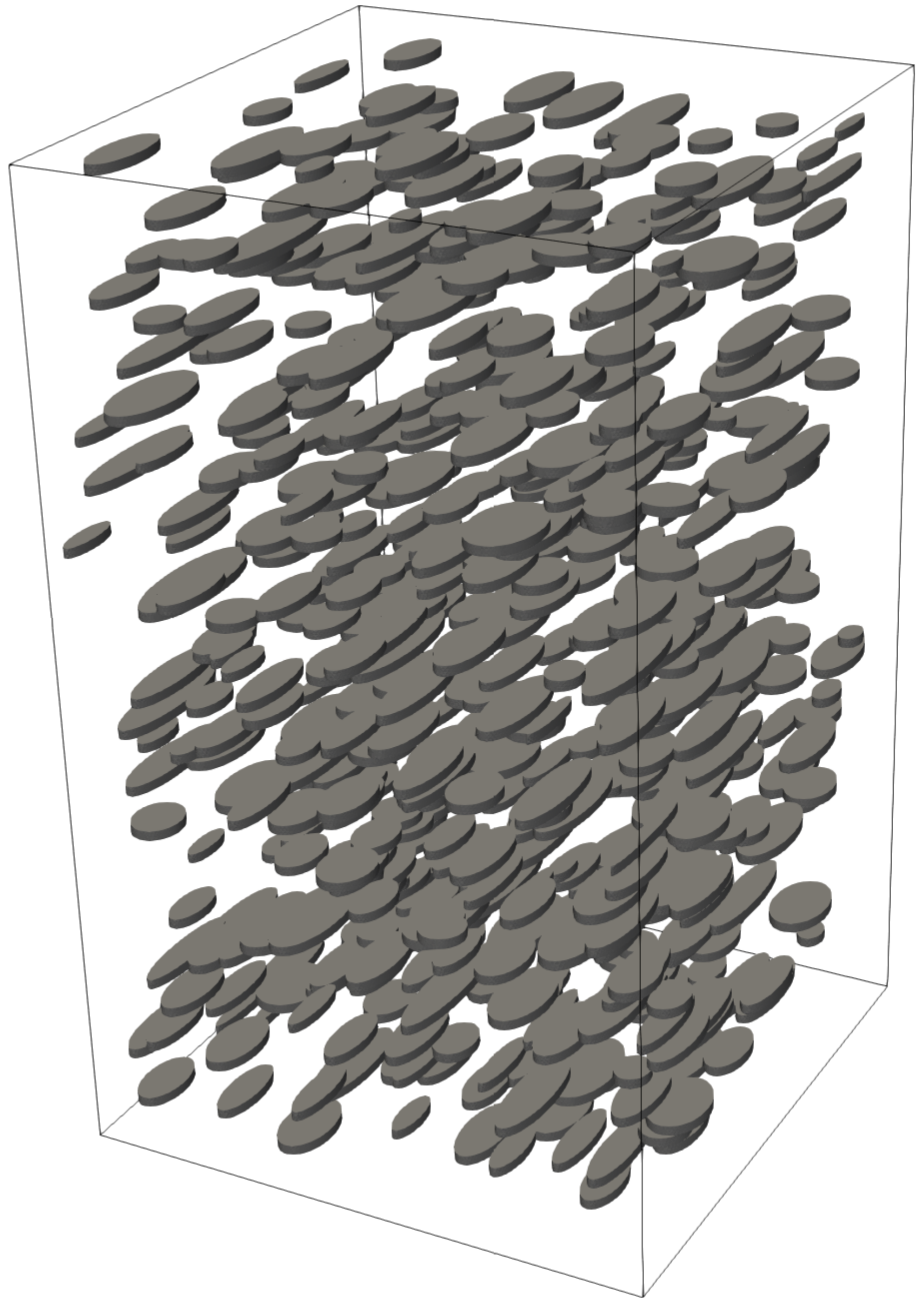
Figure 4.
Fractional Lévy motion model of permeability heterogeneity. Width parameter , Hurst parameter .
Figure 4.
Fractional Lévy motion model of permeability heterogeneity. Width parameter , Hurst parameter .

Figure 5.
Comparison of the evolution of convective mixing in isotropic and anisotropic porous media. (i) (left); and (ii) (right). Only concentrations greater than are shown. Time is dimensionless.
Figure 5.
Comparison of the evolution of convective mixing in isotropic and anisotropic porous media. (i) (left); and (ii) (right). Only concentrations greater than are shown. Time is dimensionless.

Figure 6.
Dimensionless flux across the top boundary for anisotropic homogeneous porous media in three dimensions. The dashed horizontal lines show the estimated steady flux .
Figure 6.
Dimensionless flux across the top boundary for anisotropic homogeneous porous media in three dimensions. The dashed horizontal lines show the estimated steady flux .
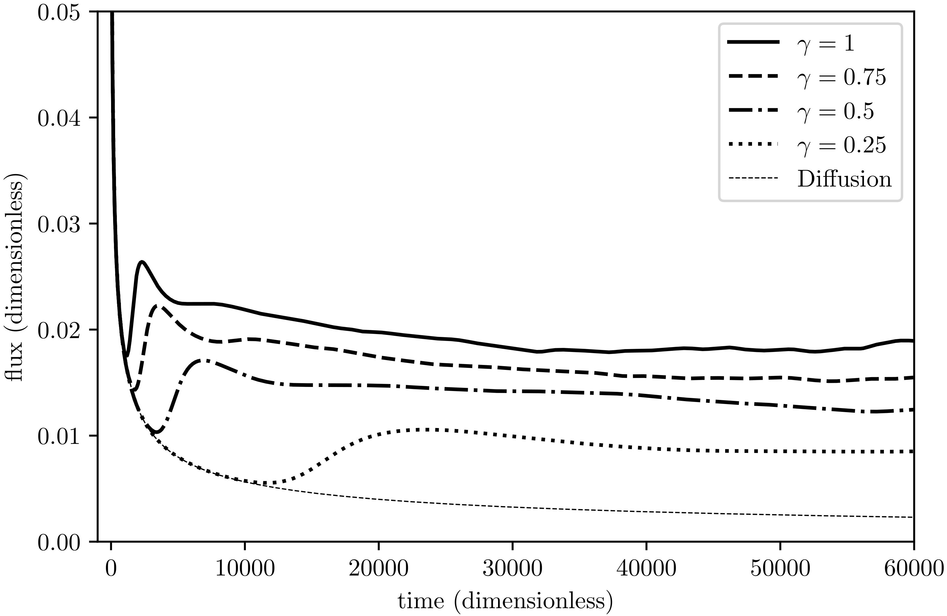
Figure 7.
Evolution of convective mixing in heterogeneous model with elliptical barriers. Barrier distribution shown in Figure 3. Only concentrations greater than are shown. Barriers are removed from the figure. Time is dimensionless.
Figure 7.
Evolution of convective mixing in heterogeneous model with elliptical barriers. Barrier distribution shown in Figure 3. Only concentrations greater than are shown. Barriers are removed from the figure. Time is dimensionless.

Figure 8.
Dimensionless flux across the top boundary for the heterogeneous model with elliptical barriers (solid line) and the equivalent anisotropic model with (dashed line).
Figure 8.
Dimensionless flux across the top boundary for the heterogeneous model with elliptical barriers (solid line) and the equivalent anisotropic model with (dashed line).
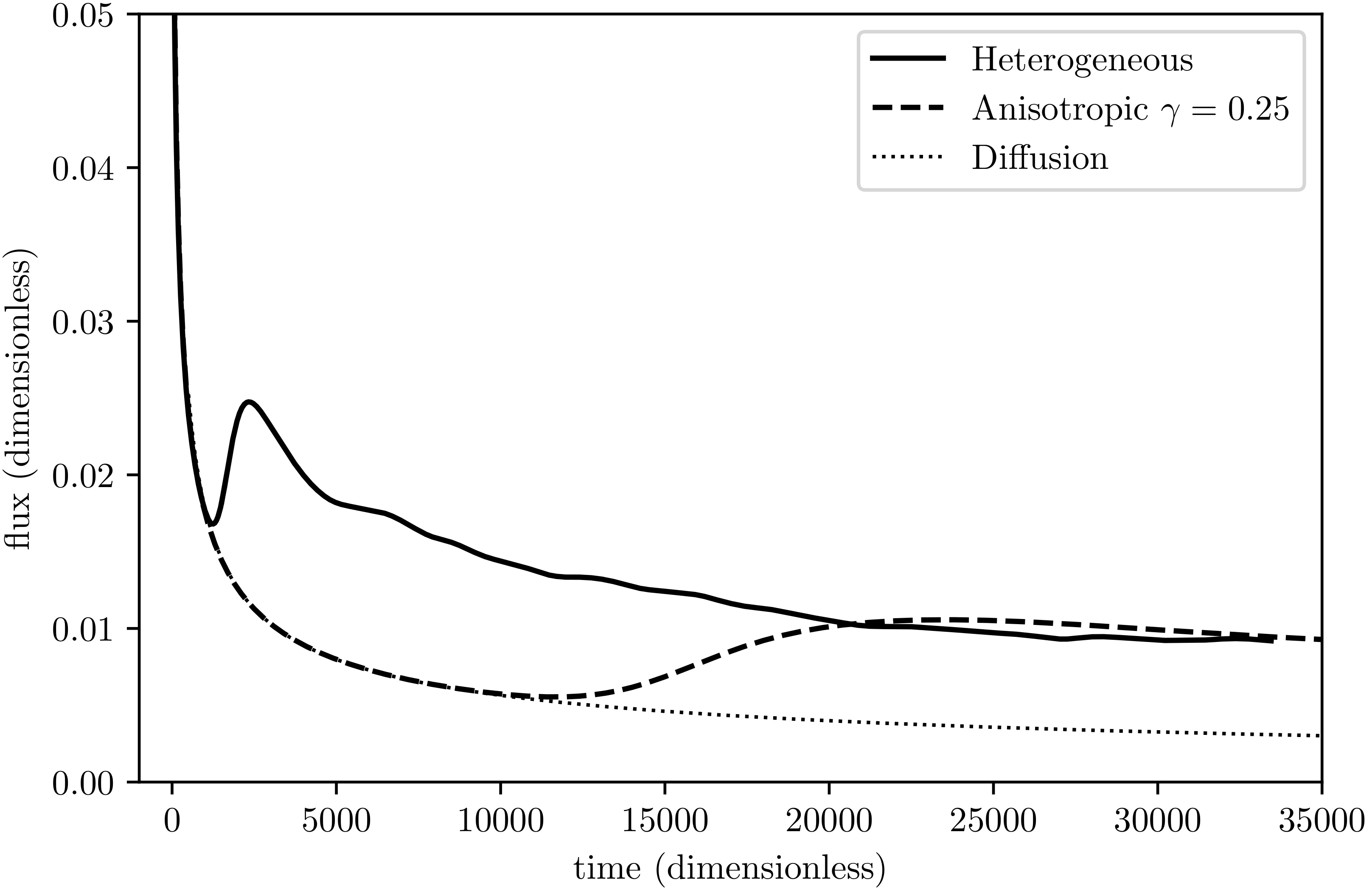
Figure 9.
Evolution of convective mixing in the heterogeneous fractional Lévy motion model (permeability heterogeneity illustrated in Figure 4. Time in seconds.
Figure 9.
Evolution of convective mixing in the heterogeneous fractional Lévy motion model (permeability heterogeneity illustrated in Figure 4. Time in seconds.

Figure 10.
Evolution of convective mixing in the heterogeneous fractional Lévy motion model for a horizontal slice 0.5 m below the top boundary. Time in seconds.
Figure 10.
Evolution of convective mixing in the heterogeneous fractional Lévy motion model for a horizontal slice 0.5 m below the top boundary. Time in seconds.
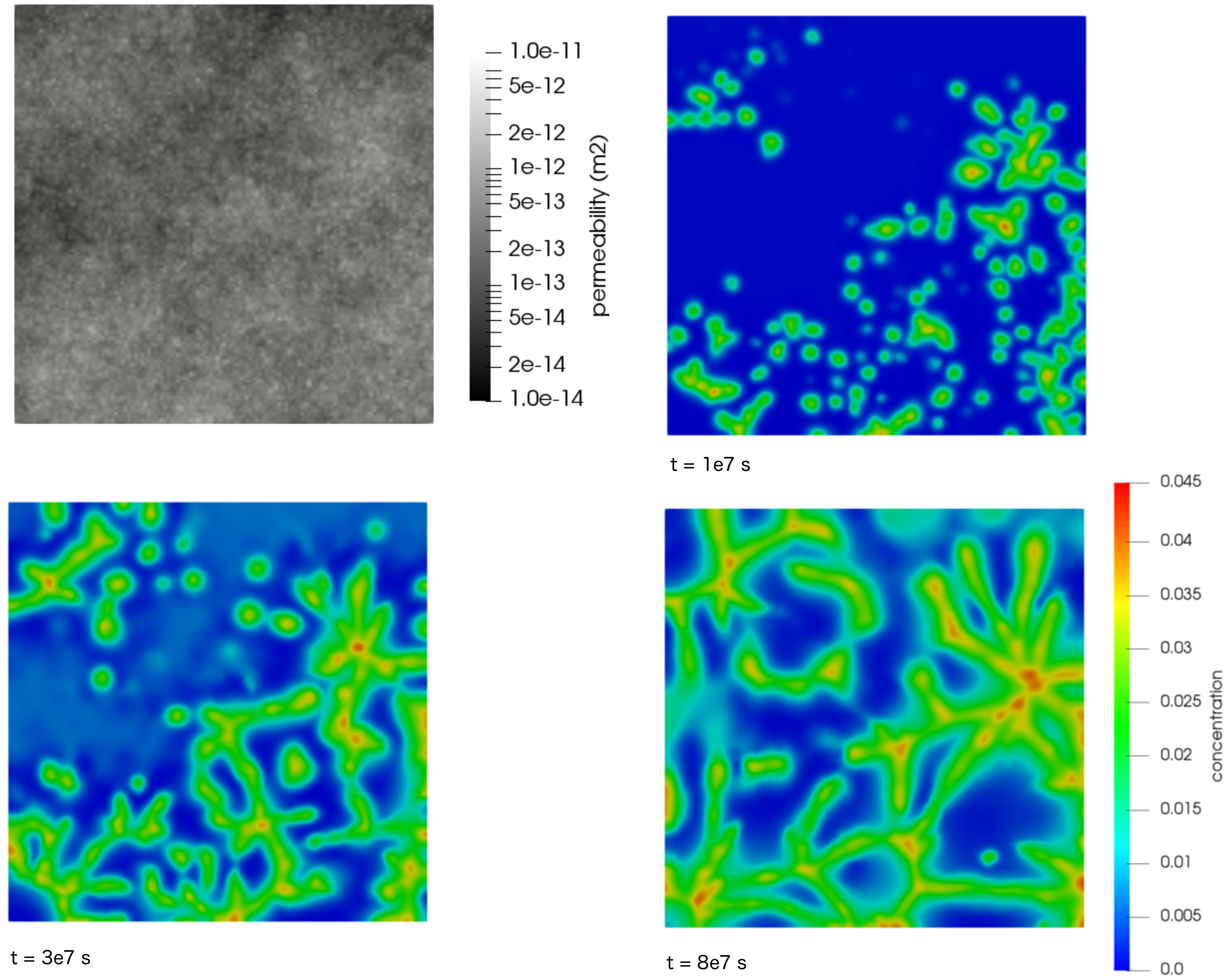
Figure 11.
Dimensionless flux across the top boundary for the fractional Lévy motion model of permeability heterogeneity (solid line) and the equivalent anisotropic model with (dashed line).
Figure 11.
Dimensionless flux across the top boundary for the fractional Lévy motion model of permeability heterogeneity (solid line) and the equivalent anisotropic model with (dashed line).
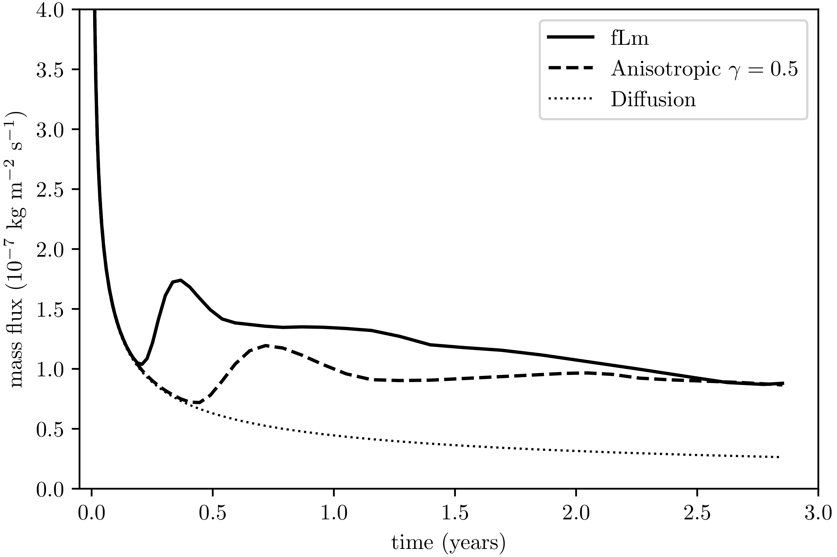
Figure 12.
Steady flux scaled by . Simulation results for anisotropic porous medium with and . Solid line is the analytical model . Dashed line is for reference. Note that the results for the barrier model (square) and the anisotropic media at are almost coincident.
Figure 12.
Steady flux scaled by . Simulation results for anisotropic porous medium with and . Solid line is the analytical model . Dashed line is for reference. Note that the results for the barrier model (square) and the anisotropic media at are almost coincident.


Table 1.
Nomenclature.
| Symbol | Definition | SI Units |
|---|---|---|
| C | Solute concentration (kg solute/kg solvent) | - |
| D | Effective diffusion coefficient | m s |
| F | Dissolution flux | kg m s |
| g | Gravity | m s |
| H | Height of model | m |
| Horizontal permeability | m | |
| Vertical permeability | m | |
| Length of model in x direction | m | |
| Length of model in y direction | m | |
| P | Pressure | Pa |
| t | Time | s |
| Fluid velocity | m s | |
| Permeability anisotropy | - | |
| Viscosity | kg m s | |
| Fluid density | kg m | |
| Porosity | - |
Table 2.
Parameters used in the dimensional simulations (representative of a low salinity aquifer at a depth of approximately 1 km).
Table 2.
Parameters used in the dimensional simulations (representative of a low salinity aquifer at a depth of approximately 1 km).
| Pressure, P | 11.4 MPa |
| Temperature, T | 59 C |
| Salt mass fraction, | |
| Porosity, | 0.25 |
| Viscosity, | kg m s |
| Unsaturated brine density, | kg m |
| Saturated brine density, | kg m |
| Saturated CO mass fraction, | |
| Effective diffusion coefficient, D | m s |
© 2018 by the authors. Licensee MDPI, Basel, Switzerland. This article is an open access article distributed under the terms and conditions of the Creative Commons Attribution (CC BY) license (http://creativecommons.org/licenses/by/4.0/).
Share and Cite
MDPI and ACS Style
Green, C.P.; Ennis-King, J. Steady Flux Regime During Convective Mixing in Three-Dimensional Heterogeneous Porous Media. Fluids 2018, 3, 58. https://doi.org/10.3390/fluids3030058
AMA Style
Green CP, Ennis-King J. Steady Flux Regime During Convective Mixing in Three-Dimensional Heterogeneous Porous Media. Fluids. 2018; 3(3):58. https://doi.org/10.3390/fluids3030058
Chicago/Turabian StyleGreen, Christopher P., and Jonathan Ennis-King. 2018. "Steady Flux Regime During Convective Mixing in Three-Dimensional Heterogeneous Porous Media" Fluids 3, no. 3: 58. https://doi.org/10.3390/fluids3030058