An Overlapping IBM-PISO Algorithm with an FFT-Based Poisson Solver for Parallel Incompressible Flow Simulations

Abstract

This study addresses computational challenges in the immersed boundary method (IBM) with the pressure implicit with split operator (PISO) algorithm for simulating incompressible flows. We introduce a novel time-step splitting method to implement communication overlapping optimization, aiming to reduce costs dominated by the pressure Poisson solver. Using a fast Fourier transform (FFT)-based approach, the Poisson equation is solved efficiently with $O(NlogN)$ complexity. Our method interleaves IBM force calculations with Poisson phases, employing asynchronous communication to overlap computation with global data exchanges. This reduces communication overhead, enhancing scalability. Validation through benchmark simulations, including flow around a cylinder and particle-laden flows, shows improved efficiency and accuracy comparable with traditional methods. Implemented in a custom C++ solver using the FFTW library, tests indicate substantial acceleration, with results showing a 40% speed-up and less than 3% deviation in drag and lift coefficients. This research provides an efficient and promising simulation tool for complex flow.

1. Introduction

The immersed boundary method (IBM) is widely employed in computational fluid dynamics (CFD). Unlike body-fitted grid methods [1], IBM avoids complex mesh generation by representing internal boundaries using force nodes that are independent of the fluid grid. This approach allows the use of uniform fluid grids even for challenges involving complex geometries, such as particle-laden flows [2] or flows around obstacles [3]. Consequently, it is extensively employed in the simulation of fluidized beds [4,5,6], biofluid mechanics [7,8], and other areas.

In simulating incompressible flows, the IBM is often integrated with the pressure implicit with split operator (PISO) algorithm [9], which calculate the pressure term via a pressure Poisson equation. As an elliptic equation, the Poisson equation introduces global dependence, allowing local perturbations to immediately affect the entire domain through the pressure field [10]. Consequently, in large-scale direct numerical simulations (DNSs), the pressure Poisson solver frequently dominates computational cost and complexity. Additionally, the main idea of IBM is using an external body force term to enforce boundary conditions [11,12,13]. Thus, in the PISO-IBM framework, the additional computational cost arises from calculating the body force at each time step [14]. Because this force calculation depends on interpolation between fluid and boundary nodes, cases with numerous interpolation nodes (e.g., particle-laden flows) can become computationally expensive.

In order to reduce computational cost, researchers focus on decreasing computational complexity and utilizing parallel computing. In terms of solving the Poisson equation, fast Fourier transform (FFT)-based algorithms are considered highly effective [15,16]. The core idea is to use the discrete Fourier transform (DFT) to convert the discrete Poisson equation into independent one-dimensional problems on different bases. This approach has two main advantages: it is well suited for parallel computation because the global elliptic equation is decomposed into multiple independent one-dimensional problems, which can be distributed across different processes; additionally, the DFT can be expedited using the FFT algorithm [17], which has a complexity of $O(NlogN)$, where N is the size of the equation. The resulting one-dimensional problems, having a tridiagonal form, can be solved using the Thomas algorithm [18], with a complexity of $O\left(N\right)$. The FFT-based algorithm has strict restrictions on geometry, as it can only be employed for equations with simple geometries. However, when coupled with IBM, its application is significantly expanded, becoming a key tool in related fields [19,20].

To accelerate IBM computation, research has focused on optimizing parallelism, as reducing the complexity of IBM calculations is not feasible. Nonetheless, parallel implementations introduce communication overhead that cannot be reduced merely by increasing the number of computational nodes. In fact, excessive nodes may exacerbate communication bottlenecks. While IBM reduces some computational costs, communication challenges remain significant for large-scale problems. One effective strategy to mitigate these bottlenecks is the overlapping method, where communication occurs concurrently with computation [21]. This approach effectively “hides” communication time by overlapping it with computational tasks. However, implementing this strategy in CFD algorithms presents a unique challenge: overlapping requires independence between computation and communication, meaning the calculated data cannot depend on the communicated data during the overlap phase.

Existing research has proposed limited optimizations for IBM-PISO algorithms in parallel environments. A common approach is to separate inner and interface regions for computation, initiate non-blocking communication for interface regions first, then compute inner regions concurrently during communication, and finally process interface regions after communication completes [22]. Some optimization strategies focus on grid-based approaches. For example, Ref. [23] employs a dual-grid for resolving fluid velocity and discrete element method (DEM) coupling while maintaining accuracy; and a coarse grid for pressure solution to accelerate large-scale computations. Additionally, numerous studies have explored performance optimizations on heterogeneous architectures, particularly focusing on multi-granularity parallelization strategies [24,25,26]. However, these methods only work for locally dependent operations like convective term calculations. They prove ineffective for global operations such as Poisson equation solving, which requires all-to-all communication.

This research introduces a novel time-step splitting method to implement overlapping optimization for the IBM-PISO algorithm. Our approach staggers the computation of the Poisson equation solution with IBM force calculations within each time step. Section 2.1 details this algorithm, which employs an FFT-based Poisson solver. Unlike classic Krylov methods [27], the FFT-based approach transforms the global equation into multiple independent sub-equations. This method offers two key advantages: (1) low computational complexity due to the efficiency of FFT and Thomas algorithms, and (2) excellent parallel scalability as sub-equations can be solved independently. While FFT-based solvers are typically restricted to simple geometries due to spectral expansion requirements, our work combines this approach with IBM to handle both simple and complex internal boundaries.

The manuscript is organized as follows: Section 2.1 presents the governing equations and solution methodology, while Section 3 details our overlapping strategy implementation. We validate the precision and the computational efficiency through multiple numerical test cases in Section 4.

2. PISO-IBM Algorithm

2.1. PISO

The incompressible non-dimensional Navier–Stokes equations are given by:

$$\begin{array}{cc}\hfill & \nabla ·{\mathit{u}}_{\mathrm{f}}=0,\hfill \\ \hfill & {\displaystyle \frac{\partial {\mathit{u}}_{\mathrm{f}}}{\partial t}}+{\mathit{u}}_{\mathrm{f}}\nabla ·{\mathit{u}}_{\mathrm{f}}=-\nabla p+{\displaystyle \frac{1}{\mathrm{Re}}}{\nabla }^2{\mathit{u}}_{\mathrm{f}}+{\mathit{f}}_{\mathrm{f}},\hfill \end{array}$$

(1)

where ${\mathit{u}}_{\mathrm{f},\mathrm{p}}$ is vector of velocity, p is pressure, and ${\mathit{f}}_{\mathrm{f},\mathrm{p}}$ is the volume force term. The subscripts $\mathrm{f}$ and $\mathrm{p}$ denote the fluid and particle phases, respectively. The external body force is omitted. Unless otherwise specified, all quantities are dimensionless throughout this paper. The Reynolds number is defined as $\mathrm{Re}={\rho }_{\mathrm{f}}UL/\mu$, with ${\rho }_{\mathrm{f}}$ being fluid density, U being the characteristic velocity, L being the characteristic length, and $\mu$ being dynamic viscosity. Quantities in the Reynolds number computation are dimensional.

In the PISO algorithm, the pressure and velocity is decoupled, such that the connection is the pressure Poisson equation. Coupled with IBM, the computation of the time advancing step is shown by

$$\begin{array}{cc}\hfill {\mathit{u}}_{\mathrm{f}}^{\ast }& ={\mathit{u}}_{\mathrm{f}}^n+\mathsf{\Delta }t(-{\mathit{u}}_{\mathrm{f}}^n·\nabla {\mathit{u}}_{\mathrm{f}}^n+{\displaystyle \frac{1}{\mathrm{Re}}}{\nabla }^2{\mathit{u}}_{\mathrm{f}}),\hfill \end{array}$$

(2a)

$$\begin{array}{cc}\hfill {\mathit{u}}_{\mathrm{f}}^{\ast \ast }& ={\mathit{u}}_{\mathrm{f}}^{\ast }+\mathsf{\Delta }t\mathcal{F}\left(\nabla ·{\mathit{u}}_{\mathrm{f}}^{\ast }\right),\hfill \end{array}$$

(2b)

$$\begin{array}{cc}\hfill {\nabla }^{2}p& =\nabla ·{\mathit{u}}_{\mathrm{f}}^{\ast \ast },\hfill \end{array}$$

(2c)

$$\begin{array}{cc}\hfill {\mathit{u}}_{\mathrm{f}}^{n+1}& ={\mathit{u}}_{\mathrm{f}}^{\ast \ast }-\nabla p,\hfill \end{array}$$

(2d)

where the superscript n denotes the temporal step and ${\mathit{u}}_{\mathrm{f}}^{\ast }$ and ${\mathit{u}}_{\mathrm{f}}^{\ast \ast }$ are the intermediate velocities for pressure correlation and IBM calculation, respectively. The computation of IBM force is denoted by ${\mathit{f}}_{\mathrm{f}}=\mathcal{F}({\mathit{u}}_{\mathrm{f}};{\mathit{x}}_{\mathrm{p}},{\mathit{x}}_{\mathrm{f}})$. In (2), we only proposed a single iteration to simplify the formula, while in the general PISO algorithm, the velocity correction via Equation (2d) requires multiple iterative steps. The pressure Poisson Equation (2c) comes from divergence-free velocity projection at each time step to maintain the divergence-free velocity, i.e., incompressibility of the flow.

2.2. FFT-Based Poisson Solving

The FFT-based Poisson solving algorithm utilizes the central difference scheme for the Poisson Equation (2c). In two dimensions, the discrete form of the Poisson equation at the $(i,j)$-th node is given by

$${\displaystyle \frac{p_{i-1,j}-2p_{i,j}+p_{i+1,j}}{\mathsf{\Delta }{x}^2}}+{\displaystyle \frac{p_{i,j-1}-2p_{i,j}+p_{i,j+1}}{\mathsf{\Delta }{y}^2}}=f_{i,j},$$

(3)

where $\mathsf{\Delta }x$ and $\mathsf{\Delta }y$ are the spatial steps in the x- and y-directions, respectively. In the PISO algorithm, the right-hand term is $f_{i,j}=\nabla ·{\mathit{u}}_{\mathrm{f}}^{\ast \ast }$. In the classic DFT framework, the pressure solution is expanded as

$$p_{i,j}=\sum _{n=1}^N{\widehat{p}}_{i,n}{q}_{nj},$$

(4)

where N is the number of nodes in the y-direction, and $q_{nj}$ are the basis functions for the spectral expansion, corresponding to the roots of unity $e^{2\pi \mathrm{i}nj/N}$ used in the DFT. As Equation (4) represents a DFT, it can be rapidly computed using the fast Fourier transform (FFT). Consequently, Equation (3) can be transformed into

$$(\delta +{\lambda }_n){\widehat{p}}_{i,n}+{\delta }_x({\widehat{p}}_{i+1,n}+{\widehat{p}}_{i-1,n})={\widehat{f}}_{i,n},$$

(5)

where $\delta =-2\left({\mathsf{\Delta }}_x^{-2}+{\mathsf{\Delta }}_y^{-2}\right)$, ${\delta }_x={\mathsf{\Delta }}_x^2{\mathsf{\Delta }}_y^{-2}$ and ${\lambda }_n=2[1-cos(2\pi n/N)]$.

Equation (5) is decoupled in n, i.e., for a given n, the equation is independent of other values of n. Therefore, (5) has been converted into independent sub-equations and is appropriate for parallel computation.

Direct application of DFT for transformation can probably lead to aliasing and sampling effects, and it is also challenging to extend to other boundary conditions such as Dirichlet and Neumann. Therefore, this study adopts spectral expansion coefficients derived from the eigentransformation of (3). These coefficients vary depending on the boundary conditions in the corresponding direction. Specifically, for Dirichlet boundary conditions, the form of $q_{nj}$ is

$$q_{nj}^{\mathrm{D}}=\sqrt{{\displaystyle \frac{2}{N+2}}}sin{\displaystyle \frac{nj\pi }{N+1}},$$

(6)

and for Neumann boundary conditions, $q_{nj}$ is

$$q_{nj}^{\mathrm{N}}=\left\{\begin{array}{cc}{\displaystyle \frac{2}{N}}sin{\displaystyle \frac{\left(2nj-j-2nN\right)}{2N}},\hfill & \hfill \left(j<N\right)\\ {\displaystyle \frac{2}{N}}sin{\displaystyle \frac{\pi }{4}},\hfill & \hfill \left(j=N\right)\end{array}\right.$$

(7)

Compared with direct DFT expansion, expressions (6) and (7) are derived directly from the matrix form of Equation (3) for the spectral space transformation. This approach avoids the aliasing and sampling effects associated with direct DFT while retaining the advantage of transforming the equation into independent sub-equations for parallel computation. Furthermore, it can be demonstrated that this process can be directly completed through FFT and vector-wise computations without increasing computational complexity.

In practical computations, compared with direct solvers, FFT-based solving algorithms involve two spatial transformation processes that include FFT. In practice, these transformations involve global communication, specifically an all-to-all process. Because other computational steps typically have a complexity no higher than $O\left(logN\right)$ on each computational unit, this global communication often becomes a bottleneck limiting computational and parallel efficiency in large-scale parallel simulations. This forms the premise for our proposed optimization based on an overlapping strategy, which will be discussed in Section 3.

2.3. IBM

The IBM approach imposes prescribed velocity conditions on arbitrary interfaces. We adopt the direct forcing scheme of Uhlmann [12], where interpolation between Eulerian and Lagrangian positions is governed by

$$\begin{array}{cc}{\tilde{\mathit{u}}}_{\mathrm{f}}\left({\mathit{x}}_{\mathrm{p}}^{\left(i\right)}\right)={\displaystyle \sum _{{\mathit{x}}_{\mathrm{f}}\in \mathsf{\Omega }}}{\mathit{u}}_{\mathrm{f}}{\delta }_h({\mathit{x}}_{\mathrm{f}}-{\mathit{x}}_{\mathrm{p}}^{\left(i\right)})h^3\hfill & \hfill 1⩽i⩽N_b,\\ {\mathit{f}}_{\mathrm{p}}\left({\mathit{x}}_{\mathrm{p}}^{\left(i\right)}\right)={\displaystyle \frac{{\mathit{u}}_{\mathrm{p}}^{\left(i\right)}-{\tilde{\mathit{u}}}_{\mathrm{f}}\left({\mathit{x}}_{\mathrm{p}}^{\left(i\right)}\right)}{\mathsf{\Delta }t}}\hfill & \hfill 1⩽i⩽N_b,\\ {\mathit{f}}_{\mathrm{f}}={\displaystyle \sum _{i=1}^{N_b}}{\mathit{f}}_{\mathrm{p}}\left({\mathit{x}}_{\mathrm{p}}^{\left(i\right)}\right){\delta }_h({\mathit{x}}_{\mathrm{f}}-{\mathit{x}}_{\mathrm{p}}^{\left(i\right)})\mathsf{\Delta }{V}^{\left(i\right)}\hfill & \hfill \forall x_{\mathrm{f}}\in \mathsf{\Omega },\end{array}$$

(8)

where force points are indexed by superscript i, $N_b$ is number of force points, ${\delta }_h$ is a kernel function used for interpolation, and the radius of the IBM kernel function is denoted as $d_h$, h is mesh width. The integration domain $\mathsf{\Omega }$ represents the fluid region within a distance $d_h$ from the force point. ${\tilde{\mathit{u}}}_{\mathrm{f}}$ is the interpolated fluid velocity located in force points, $\mathsf{\Delta }t$ is the time step, and $\mathsf{\Delta }{V}^{\left(i\right)}$ is the discrete volume associated with each force point such that the union of all these volumes forms a thin shell (of thickness equal to one mesh width). If the force point is uniformly distributed, then all $\mathsf{\Delta }{V}^{\left(i\right)}$ are equal.

3. Overlapping Strategy

The proposed overlapping strategy to accelerate the computation of (8) focuses on parallel implementation, with the parallelization strategy detailed in this section. For parallel computation, we employ a one-dimensional (slab) domain decomposition of the 2D fluid domain, partitioning the computational domain uniformly along the y-axis to optimize load balancing. Extending this approach to 3D configurations is conceptually straightforward, requiring only algorithmic generalization without altering the core logic of the overlapping scheme.

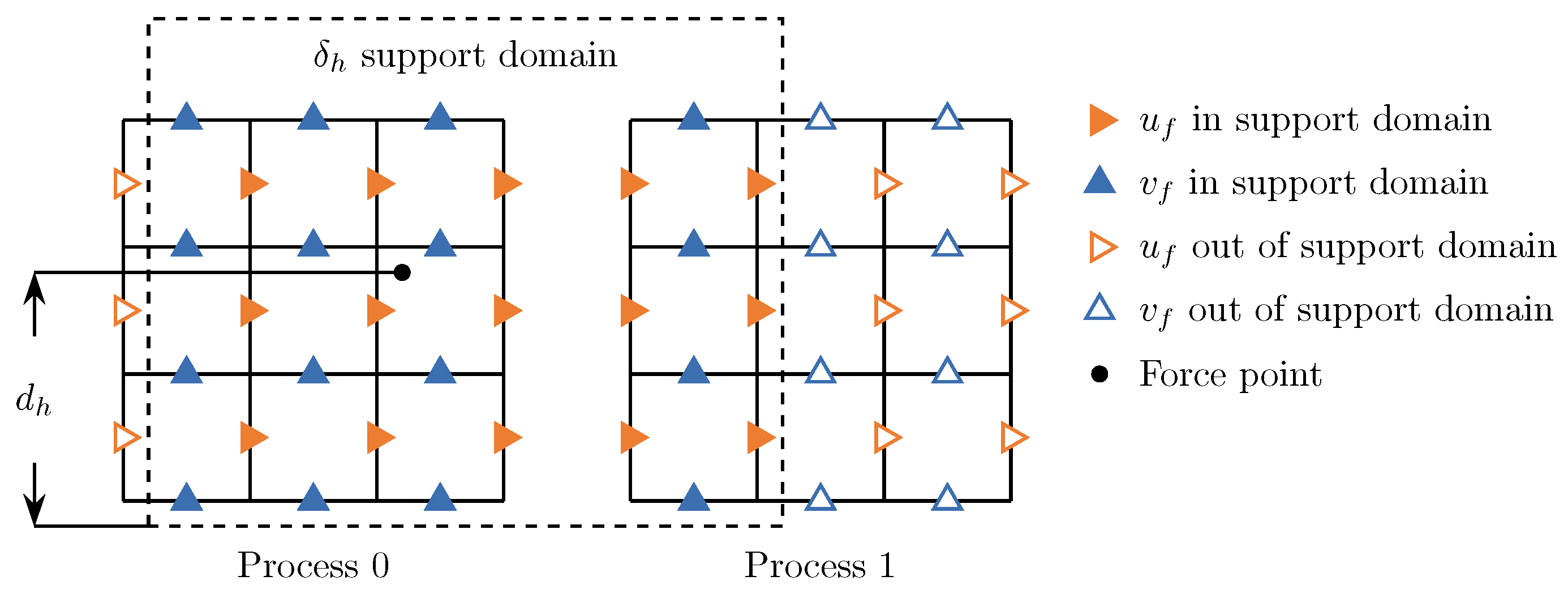
As mentioned in Section 2.1, the Poisson equation is discretized using the finite difference method (FDM). In this research, the incompressible Navier–Stokes equations are discretized by FDM with a staggered grid, where discrete nodes for velocity in the x- and y-directions and pressure are located at different positions, as shown in Figure 1. Furthermore, while employing one-dimensional (slab) domain decomposition in FDM-IBM, updating a grid point requires information from neighboring points following a specific dependency pattern known as the finite difference stencil. The stencil of a force point defines its dependence on adjacent Eulerian fluid points, determined by the support region of the kernel function ${\delta }_h$.

As shown in Figure 1, in the parallel implementation of IBM, certain force points near the slab boundary may have stencils extending beyond the local process domain. For such points, the stencil includes Eulerian velocity points from both the local process and adjacent processes. Consequently, the local process requires Eulerian velocity and Lagrangian force data from near-boundary regions of neighboring processes.

In the parallelization implementation, each process maintains buffer regions on both sides of its local slab boundary. These buffers receive the necessary data for stencil computation from neighboring processes. When the support region spans the boundary between two processes, both the calculation of the force on the Lagrangian point ${\mathit{f}}_{\mathrm{p}}$ and the body force ${\mathit{f}}_{\mathrm{f}}$ require data from neighboring processes. Consequently, two buffer synchronizations are necessary in the Lagrangian-to-Eulerian force calculation:

• Eulerian velocity increment synchronization: The local process computes the force contribution ${\mathit{f}}_{\mathrm{f}}$ from near-boundary force points affecting neighboring processes and transmits it via MPI to the neighbor’s buffer, where it is applied to the Eulerian velocity field.
• Lagrangian force point synchronization: The local process sends boundary force points ${\mathit{f}}_{\mathrm{p}}\left({\mathit{x}}_{\mathrm{p}}^{\left(i\right)}\right)$ directly to the neighbor’s buffer, allowing each process to independently compute ${\mathit{f}}_{\mathrm{f}}$.

First subroutine incurs communication costs proportional to the grid size, while the second scales with the number of force points. The choice between these two methods depends on the specific simulation case. For example, when simulating a fluid with many particles, resulting in a large number of force points, the second subroutine would be more advantageous.

In general, the overlapping strategy typically involves overlapping the calculations of buffers and interior points. However, when the number of processes is large, the buffer size may be insufficient to match the interior points, resulting in communication times that do not overlap with computation times. The new overlapping strategy proposed in this paper focuses on overlapping communication in the FFT-based Poisson solving and buffer synchronization, rather than within a single IBM subroutine.

Specifically, as described in (5), the FFT-based Poisson solver involves two critical global communication (all-to-all) processes. This involves transformations from physical space to Fourier space and vice versa, implemented as two transposition processes: transforming an array indexed by the y-direction to one indexed by n, each constituting an all-to-all global communication process, with a similar inverse transformation. Therefore, the proposed overlapping strategy can be understood as overlapping the two communication processes within IBM with the two in the Poisson solver. The detailed implementation process is described in Algorithm 1.

Algorithm 1 Overlapping Fluid–Particle Coupling Algorithm with CPU-IO Parallelism
1: Solve momentum equation:
2: Parallel Execution:
Computation process:	Communication process:
1. Transformation by FFT	1. Synchronize $u_{\mathrm{f}}$ buffer data
2. Update ${\tilde{\mathit{u}}}_{\mathrm{f}}\left({\mathit{x}}_{\mathrm{p}}^{\left(i\right)}\right)$ and ${\mathit{f}}_{\mathrm{p}}\left({\mathit{x}}_{\mathrm{p}}^{\left(i\right)}\right)$	2. Transpose data from $x-y$ to $y-x$ direction
3. Apply chasing method	3. Synchronize ${\mathit{f}}_{\mathrm{p}}\left({\mathit{x}}_{\mathrm{p}}^{\left(i\right)}\right)$ buffer data
for pressure solution
4. Update ${\mathit{f}}_{\mathrm{f}}$ and velocity ${\mathit{u}}_{\mathrm{f}}$	4. Transpose data from $y-x$ to $x-y$ direction
5. Inverse transformation by IFFT
3: Combine results from both processes and solve pressure equation:

In the classic PISO algorithm shown in (2), the computation and communication subroutines for both the IBM and Poisson solving are executed sequentially. In contrast, the algorithm based on the proposed overlapping strategy interleaves the computation phases of the IBM and Poisson solving, as demonstrated in Algorithm 1. The time advancement process of the overlapping algorithm can be expressed as

$$\begin{array}{cc}\hfill {\nabla }^{2}p& =\nabla ·{\mathit{u}}_{\mathrm{f}}^{\ast },\hfill \end{array}$$

(9a)

$$\begin{array}{cc}\hfill {\mathit{u}}_{\mathrm{f}}^{n+1}& ={\mathit{u}}_{\mathrm{f}}^{\ast }+\mathsf{\Delta }t\mathcal{F}\left(\nabla ·{\mathit{u}}_{\mathrm{f}}^{\ast }\right)-\nabla p,\hfill \end{array}$$

(9b)

The intermediate velocity ${\mathit{u}}_{\mathrm{f}}^{\ast }$ is calculated from the advective and dissipative terms, consistent with (2a). It is important to note that both (2) and (9) are based on a first-order forward scheme for simplicity. However, in transient simulations, to maintain an acceptable time step, a low-order time advancement scheme is not always reliable. In the actual implementation, as seen in the numerical results in Section 4, we employ the 4th-order Runge–Kutta algorithm.

4. Numerical Results

In this section, we validate the precision of our proposed algorithm and assess the impact of the overlapping algorithm on the accuracy of transient flow simulations. Specifically, we compare the numerical solution with an analytically constructed solution of the incompressible Navier–Stokes equations. For the well-known benchmark problem of two-dimensional flow around a cylinder, we compare the numerical results from our solver, which incorporates the proposed overlapping method, with solutions obtained using the classic method. In this context, we evaluate computational efficiency using different numbers of MPI processes and assess parallel computation acceleration. To analyze the speed-up effect of the proposed overlapping method, we construct a particle-laden flow scenario with varying numbers of particles and compare the results with those obtained from the classic algorithm in terms of computational efficiency.

All numerical results were obtained using an in-house solver developed in C++. The open-source FFT library FFTW [28], known for its high efficiency, is the only third-party library used in our development. Based on this self-developed solver, all numerical results were achieved, and all parallel tests were conducted on the CPU parallel computational platform described in Section 4.2.

4.1. Precision Validation

A constructed analytical solution is employed to evaluate the accuracy of the algorithm. This is the so-called method of manufactured solution, which is believed to be a severe test for numerical computations [29,30]. The solution is defined as

$$\begin{array}{cc}\hfill u& =C_1{\varphi }^2{\displaystyle \frac{\partial \varphi }{\partial y}},\hfill \\ \hfill v& =-C_1{\varphi }^2{\displaystyle \frac{\partial \varphi }{\partial x}},\hfill \\ \hfill p& =\zeta {\varphi }^2\hfill \end{array}$$

(10)

where

$$\begin{array}{cc}\hfill {\varphi }_0\left(x,y\right)& =\left(x-x^2\right)\left(y-y^2\right)\left[{\left(x-{\displaystyle \frac{1}{2}}\right)}^2+{\left(y-{\displaystyle \frac{1}{2}}\right)}^2-r^2\right],\hfill \\ \hfill \psi \left(x,y\right)& =sin\left(\omega t\right)\left(x-{\displaystyle \frac{1}{2}}\right)+cos\left(\omega t\right)\left(y-{\displaystyle \frac{1}{2}}\right),\hfill \\ \hfill \varphi \left(x,y\right)& ={\varphi }_0\psi .\hfill \end{array}$$

(11)

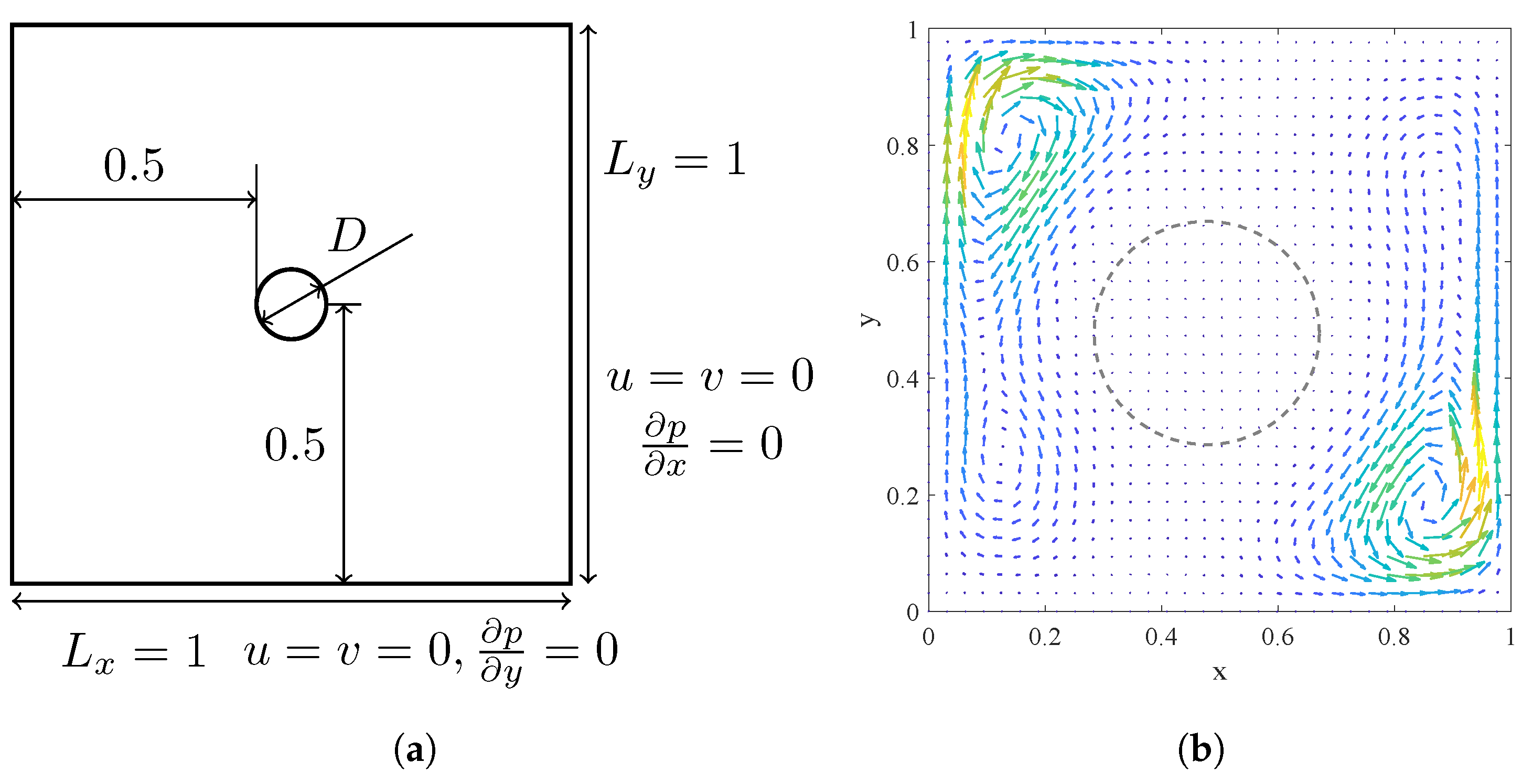
Solution ${\mathit{u}}_{\mathrm{f}}=\left[u\left(x,y\right),v\left(x,y\right)\right]$ satisfies the incompressible condition. Figure 2a depicts the geometry of the analytical solution, which consists of a stationary square outer boundary and a circular inner boundary. Both boundaries enforce no-slip wall conditions. The circular of diameter $D=0.4$ is centered at $(0.5,0.5)$, with the outer square boundary extending from $(0,0)$ to $(1,1)$.

We compare velocity results at $t=1$ from the overlapping algorithm, labeled as “overlapping” in Figure 3, with those obtained from the classic sequential algorithm, labeled as “classic,” across various spatial discretizations.

As shown in Figure 3, the discretization accuracy is between first and second order. This is consistent with the results of the classic algorithm in both the entire field and at nodes surrounding the obstacle. The overlapping algorithm does not affect the order of accuracy, suggesting that the overlapping strategy retains similar computational precision.

4.2. Flow Around a Cylinder

Flow around a cylinder is a classical benchmark problem. To assess the reliability in transient flow and computational efficiency of the proposed method, the setup depicted in Figure 4 is used. The left boundary serves as an inlet with a velocity of 1, while the top and bottom boundaries are stationary walls, and the outlet boundary is treated as a fully developed flow boundary. The computational domain has the dimensionless dimensions $L_x=L_y=8$ with a cylinder of diameter $D=0.3$ positioned at $(1.85,4)$. The Reynolds number is defined as $\mathrm{Re}={\rho }_f{u}_{in}D/\mu =100,1000$, where inlet velocity $u_{in}=1$. The computational grid uses uniform spacing of $\mathsf{\Delta }x=\mathsf{\Delta }y=1/128$ for $\mathrm{Re}=100$ cases and $\mathsf{\Delta }x=\mathsf{\Delta }y=1/512$ for $\mathrm{Re}=1000$ cases.

Drag coefficient $C_d=2F_d/\left(\rho u^2\pi r^2\right)$, lift coefficient $C_l=2F_l/\left(\rho u^2\pi r^2\right)$, and Strouhal number $\mathrm{St}=f_{v}D/u$ are calculated, where $F_d,F_l$ is the drag force and lift force on cylinder, u is the inlet velocity, r is the cylinder radius, $f_v$ is the frequency of vortex shedding.

Table 1. Comparison of average drag coefficient ${\overline{C}}_d$, the amplitude of the drag and lift fluctuation $C_d^{\prime },C_l^{\prime }$, and Strouhal number $\mathrm{St}$ in the case of a flow past stationary cylinder.

Re	Method	${\overline{\mathbf{C}}}_{\mathbf{d}}$	${\mathbf{C}}_{\mathbf{d}}^{\prime }$	${\mathbf{C}}_{\mathbf{l}}^{\prime }$	St	${\overline{\mathbf{C}}}_{\mathbf{d}}$ Error
100	Original	1.522	±0.007	±0.248	0.167	1.40%
	Overlapping	1.550	±0.007	±0.222	0.167	3.26%
	Reference [12]	1.501	±0.011	±0.349	0.172
1000	Original	1.753	±0.201	±1.129	0.260	8.28%
	Overlapping	1.735	±0.171	±0.971	0.260	7.16%
	Reference [31]	1.619	±0.156	±1.372	0.232

shows that all quantities are found in good agreement with references.

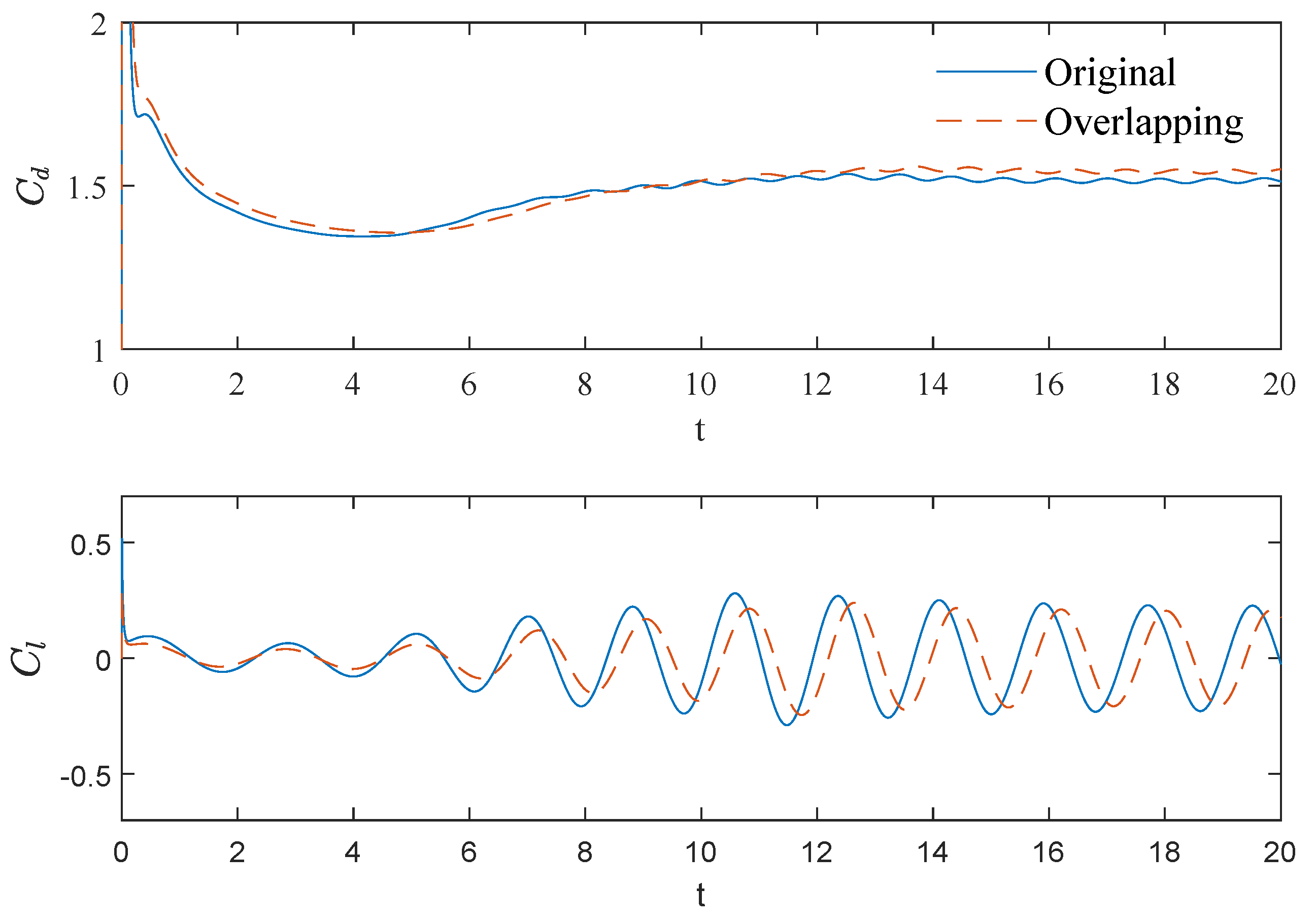
The time evolution of drag and lift coefficients are depicted in Figure 5. It can be seen that both forces settle to a regular sinusoidal function after vortex shedding becoming stable. Comparing the two algorithms, there are small amplitude and phase differences between these two curves. As shown in Table 1, the overlapping algorithm predicts the mean drag coefficient with a maximum deviation of 7.16% comparing with reference data. This discrepancy, which falls within acceptable limits, can be primarily attributed to algorithmic accuracy and geometric parameters of the flow field. The drag and lift coefficient phase shift results from numerical velocity perturbations affecting vortex shedding initiation. Common practice in the literature involves initial perturbations (random velocities across the fluid domain or cylinder rotation) to trigger vortices earlier. Although these methods modify the exact onset timing, the essential vortex dynamics remain unchanged.

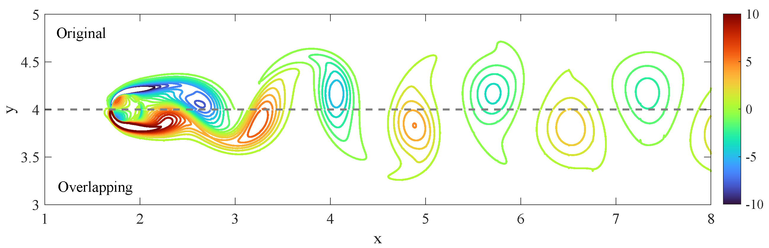
The vorticity distribution, indicative of the transient flow structures like the Kármán vortex street, is shown in Figure 6. The upper half depicts the results from the classic algorithm, while the lower half shows results from our proposed algorithm. It is apparent that the vorticity distributions are very similar, with almost continuous contour lines, indicating consistency between the two approaches.

To evaluate the optimization effect of the proposed algorithm, computational efficiency was compared between our proposed method and the classic algorithm on a server with two CPUs. Detailed software and hardware configurations are provided in

Table 2. Hardware and software specifications of the efficiency test platform.

Parameter	Value
CPU Model	Intel(R) Xeon(R) Gold 6230R @ 2.10 GHz
CPU Cores (per CPU)	26
Number of CPUs	2
RAM	256 GB
C++ Compiler	Intel OneAPI (gcc version 7.2.0)
FFTW Library	3.3.10

.

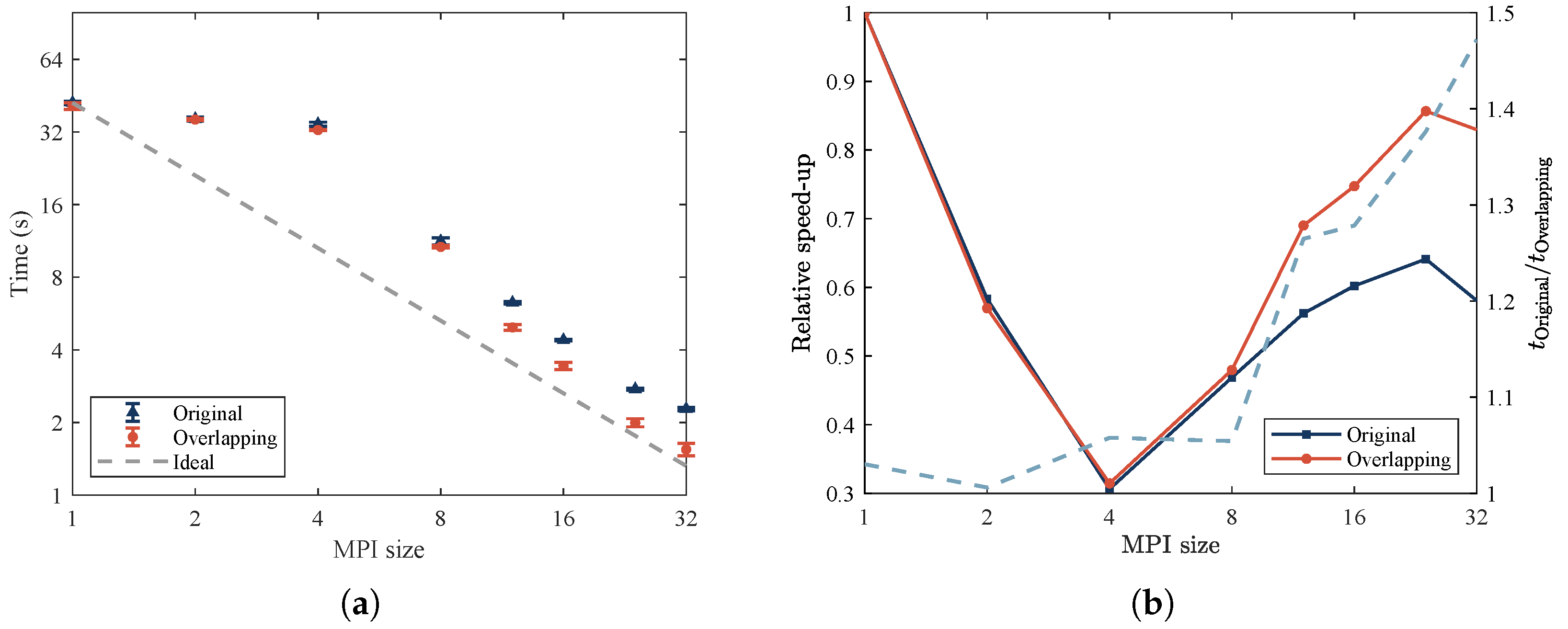
Parallel efficiency is assessed by measuring computational time across various numbers of MPI processes, as shown in Figure 7. The primary aim is to evaluate optimizations in parallel computation using relative speed-up R, defined by

$$R\left(n\right)={\displaystyle \frac{{t|}_{n_{\mathrm{p}}=1}}{{n\times t|}_{n_{\mathrm{p}}=n}}},$$

(12)

where ${t|}_{n_{\mathrm{p}}=n}$ is the computational time for n MPI processes. The parallelization is implemented using MPI in C++, ensuring that the number of MPI processes equals the number of CPU cores. The parallel efficiency is tested up to 32 CPU cores, as indicated in Figure 7.

In Figure 7a, the gray dashed line represents ideal computational efficiency, where n CPU cores yield n times speed-up. The pale line demonstrates that computational efficiency improves continuously across different core counts.

To further analyze parallel efficiency, Figure 7b compares relative speed-up between the classic algorithm and our proposed method. The proposed algorithm consistently demonstrates higher efficiency, particularly as CPU cores increase. When CPU cores exceed 8, the proposed algorithm achieves over 40% speed-up compared with the classic method, aligning with expectations that the overlapping strategy increases computational efficiency with more CPU cores.

4.3. Multiple Particles in Cavity

To evaluate the efficacy of our proposed optimization method, we present a case of multiple particles in cavity. The case setting is following with the research of particle-laden flow by Zhi-Gang Feng and Efstathios E. Michaelides [32], which is a well-studied problem in computational fluid dynamics, often using the IBM approach to simulate the interaction between the flow and solid particles [33].

In this efficiency experiment, the domain is a box with dimensions $2\mathrm{cm}\times 2\mathrm{cm}$, with each circular particle having a diameter of $D=0.625\mathrm{cm}$. The computational grid uses a uniform spacing of $\mathsf{\Delta }x=\mathsf{\Delta }y=1/256\mathrm{cm}$. The mesh resolution is set at 16D to ensure that the particle dynamics are fully resolved. The fluid density is ${\rho }_{\mathrm{f}}=1{\mathrm{g}/\mathrm{cm}}^3$, and the particle-to-fluid density ratio is $1.01$. The fluid’s kinematic viscosity is $1\mathrm{g}/\mathrm{ms}$. Particles are precisely positioned in a uniform grid pattern to avoid collision.

The particles are initialized with randomly generated unit velocities: in the x-direction, the velocity may be either positive or negative, while in the y-direction, it is constrained to be positive. For simplicity, particle advection is disabled, and the velocities are utilized solely for the IBM computations. The fluid driving force is thus entirely derived from the velocity difference between the particles and the flow field. Disabling particle advection allows us to focus on evaluating the performance of the overlapping algorithm in handling a large number of force points, without the additional complexity of particle motion or collision dynamics.

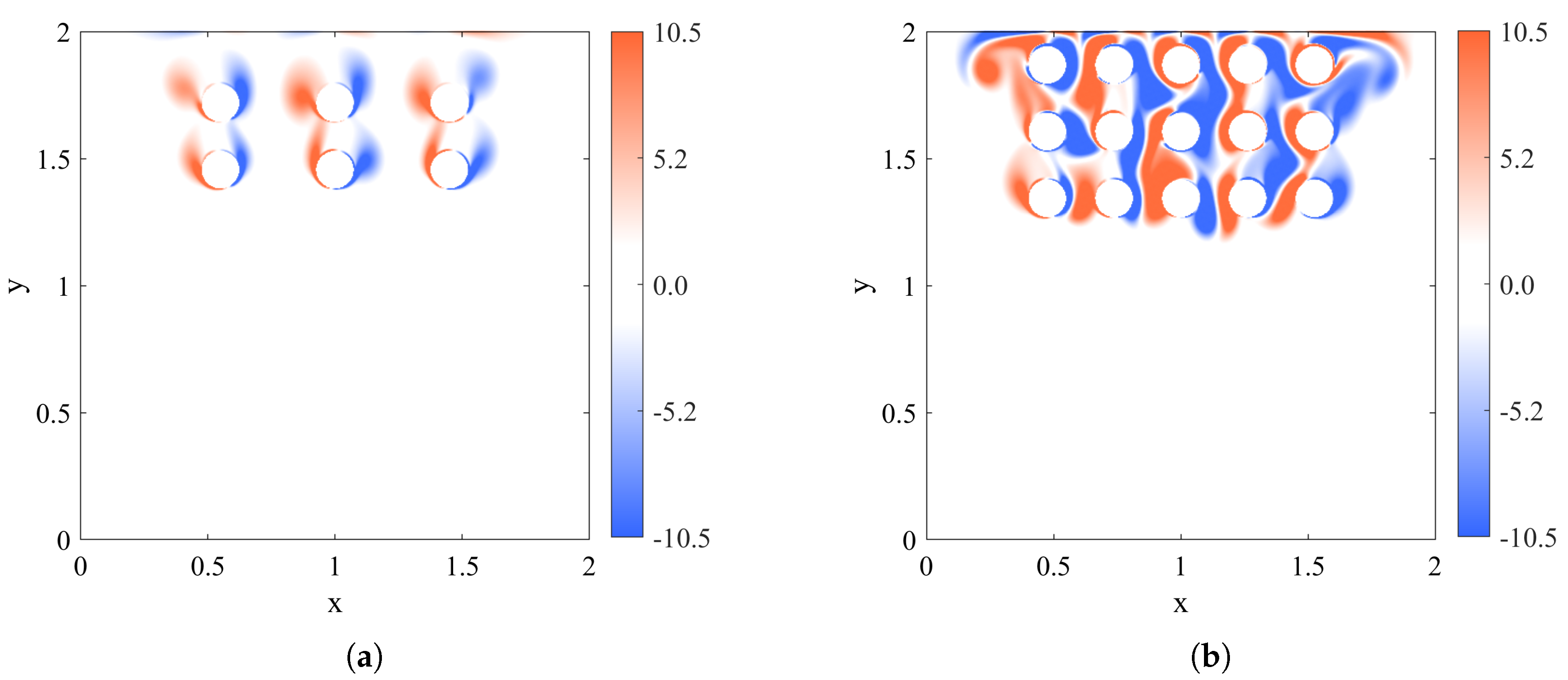
Figure 8 illustrates the vorticity field in the particle-laden flow, offering a visual insight into the flow structures. It is imperative to note that this vorticity illustration is primarily for demonstration. The particle counts used for efficiency experiment, as depicted in Figure 9, are significantly larger.

In this efficiency experiment, simulations were conducted over 200 timesteps, and the average computational time per step was calculated from the final 100 timesteps, effectively removing any initialization transients to provide a robust measure of steady-state performance.

Figure 9 highlights the computational efficiency of both the standard and the overlapping methods relative to particle count. The plot clearly indicates that the computational cost of the standard method escalates with an increase in particle count, mirroring the intensifying computational demand of the IBM process. Conversely, the overlapping method reveals a distinct trend. The communication overhead for processes substantially diminishes the increased cost of IBM calculations, resulting in very stable computational time with an increasing number of particles.

It is theoretically anticipated that the computational cost of the overlapping method will also rise beyond a certain particle count threshold. Nevertheless, in this study, the particle numbers do not exceed this limit, as the maximum particle counts already occupy a significant part of the computational domain.

5. Conclusions

To promote the computational efficiency of the IBM-PISO algorithm in parallel computation, this study proposes an overlapping-based parallel optimization strategy. The distinctive feature of the proposed method, compared with traditional approaches, lies in its modified time-stepping scheme, which interleaves the solution of the FFT-based pressure Poisson equation and the IBM force calculation. By employing a communication–computation overlap technique, communication overhead is effectively hidden during transient simulations, thereby significantly accelerating the PISO algorithm in parallel computation. An in-house code was developed and employed to conduct numerical evaluations of the proposed method on parallel platforms, including assessments against a manufactured analytical solution and the benchmark problem of flow around a circular cylinder. The results demonstrate that the proposed method exhibits significantly superior computational efficiency compared with the classic sequentially executed IBM-PISO scheme, particularly when employing a large number of CPU cores and when dealing with complex immersed boundaries characterized by a high density of IBM force points. Consequently, this method is particularly well suited for fluid dynamics problems with complex immersed boundaries, especially fluid–structure interaction (FSI) problems. The developed algorithm offers a valuable and efficient alternative for addressing these challenging simulations.

To further validate the capabilities of our proposed overlapping algorithm, comprehensive numerical experiments need to be conducted to assess its performance in handling complex geometries, moving boundaries, and elastic boundary conditions. Additionally, the proposed algorithm requires systematic validation for various FSI problems.

While our current IBM implementation builds upon the basic direct forcing method, we recognize opportunities to incorporate more advanced IBM variants. These include the multiple direct forcing method [34], Poisson equation modification techniques [35] for enhanced divergence-free condition enforcement at boundaries, and moving least squares methods for greater interpolation stability [36]. Integrating these advanced methods with our FFT-based overlapping strategy represents a promising avenue for future research.

Due to the structural limitations of the Poisson equation matrix, FFT-based solvers are restricted to rectangular domains. As a result, our proposed overlapping algorithm, which builds upon FFT-based Poisson solvers, currently shares the same limitation. Recent studies have explored extensions to curvilinear orthogonal coordinates [37] and dimensionality reduction strategies, where FFT is applied along a selected direction and the reduced subproblems are solved using multigrid methods [38]. Nevertheless, these approaches remain fundamentally constrained by the underlying matrix structure. Addressing this limitation will be an important direction for future work.