Evaluation of Conceptual Hydrological Models in Data Scarce Region of the Upper Blue Nile Basin: Case of the Upper Guder Catchment

Department of Agricultural and Bioprocess Engineering, Ambo University, P.O. BOX 19, Ambo, Ethiopia
Hydrology 2017, 4(4), 59; https://doi.org/10.3390/hydrology4040059
Submission received: 5 October 2017
/
Revised: 1 December 2017
/
Accepted: 1 December 2017
/
Published: 6 December 2017
Abstract
:The prediction of dominant hydrological processes is imperative with the available information in data scarce regions by means of the lumped hydrological models for the purpose of water resource management. This study is aims at an intercomparison of the performances of the conceptual hydrological models in predicting streamflow. The Veralgemeend Conceptueel Hydrologisch (VHM) and NedborAfstromnings Model (NAM) lumped rainfall–runoff models were manually calibrated and validated for periods of 1 January 1990–31 December 2000 and 1 January 2001–31 December 2005, respectively. Some of the parameters of the models (i.e., recession constants of subflow components) were estimated from the preprocessing of the streamflow data using the Water Engineering Time Series PROcessing tool (WETSPRO). These parameters were used for the initial model setup and subjected to slight adjustments during calibration. The performances of the models were evaluated by graphical and statistical means. The results depicted that the models reproduced the streamflow in a good way and that the overall shape of the hydrograph was properly captured. A Nash Sutcliffe efficiency (NSE) of 0.71 and 0.67 were obtained during calibration, whereas, for the validation period, NSE of 0.6 and 0.58 were obtained for VHM and NAM, respectively. The water balance discrepancy (WBD) of −0.1% and −13.7% were achieved for calibration, while −17% and −9% were acquired during validation for VHM and NAM, respectively. Though the models underestimated the high flows, the low flows were relatively well simulated. From the overall evaluation of the models, it is noted that the NAM model performed better than the VHM model in predicting the flow. In conclusion, the models can be used for water resource management and planning with precautions for extreme flow.
1. Introduction
The Upper Blue Nile basin is one of the basins which has been affected by climate change, as well as catchment characteristics alteration due to the natural or anthropogenic activities, which may lead to extreme events such as drought and flood [1,2]. These chronic factors modify the normal functioning of the hydrologic cycle of the basin, which in turn alters the hydrological processes in the basin [3]. Thus, for successful management and planning of water resources, a thorough understanding of the hydrological processes of the basin is crucial.
Hydrological models have been widely applied for comprehending these processes over the past few decades [4,5]. The models represent the catchment processes in a simplified way. They can be categorized as distributed and lumped models based on the way they represent the hydrological processes in the catchment [6].
The distributed hydrological models characterize the catchment in details, but intensive data are required which are not available in most developing countries [7]. However, if the catchment data (i.e., topography, soil and land use maps) are available in addition to precipitation and evapotranspiration information, they have a high importance in reproducing the runoff for the catchments with no streamflow record to assist water infrastructure investments [8,9,10]. Distributed hydrological models represent the heterogeneity of the catchment by considering the spatial variability of hydrometeorological variables, topography, geology, soil type and land use. Nevertheless, their complexity, long computation time and enormous data requirement lead them to have a limited practicality in most contexts [11]. Typical examples include the System Hydrologique European (SHE) model [12] and Institute of Hydrology Distributed Model (IHDM) [13].
On the other hand, lumped hydrological models represent the catchment as a single unit. They are characterized by minimal data requirement which is averaged over the catchment. In these types of models, the parameter values are determined through calibration, not from the physical behaviors of the catchment [9]. In addition, the spatial inhomogeneities of the input variables and parameters are not represented, which limit their capability to simulate all of the hydrological processes of the catchment. Thus, only the dominant ones are properly described. Examples of these models include the Hydrologiska Byrans Vattenavdelning (HBV) [14], Sacramento soil moisture accounting model [15] and physically-based runoff production model (TOPMODEL) [16]. For the study catchment, only hydrometeorological data are available. Thus, preference was given to lumped hydrological models as they only require hydrometeorological data as input for hydrological simulation.
The understanding of hydrological processes at catchment scale is very limited in the Upper Blue Nile basin. Most of the hydrological investigations have been focused on the basin scale with the outlet at ElDiem near the Ethio-Sudanese border and the head water of the basin, particularly the Tana basin [17]. In addition, most of the studies conducted were based on a single conceptual hydrological model. Relying on single lumped hydrological model may lead to incorrect decisions for water resource management and planning, particularly in a data scarce basin such as the Upper Blue Nile basin, due to uncertainty in the model [18,19]. Thus, studies based on the use of multiple models may give a more concrete basis for decision making.
Moreover, only limited studies have been reported in the literature on quantifying the hydrological processes of the catchments in the southern and southwestern parts of the Upper Blue Nile basin [17,20,21]. Thus, this study is conducted with objectives to (1) predict the stream flow of the Upper Guder catchment in southwestern of the Upper Blue Nile basin; and (2) to intercompare the performances of the models in predicting the flow.
2. Materials and Methods
2.1. Study Catchment
The upper Guder catchment is a sub-basin of the Guder basin in the upper Blue Nile basin which has an area of about 524 km2 and is located within latitude 8°45′ and 9°22′ N and longitude 37°30′ and 37°70′ E (Figure 1). The catchment was delineated from the Digital Elevation Model (DEM) obtained from the Shuttle Radar Topographic Mission (SRTM) acquired from the Consortium for Spatial Information (CGIR-CSI) website (http://srtm.csi.cgiar.org/, last accessed on 4 June 2017). The Guder River starts from the mountainous area of South of Ambo and Guder towns at an elevation of 3000 m above sea level. It collects water from a number of streams (i.e., Huluka, Fatto, Indris and Debis) along its way to the lower Guder, where it meets the Blue Nile river. The catchment obtains most of its rainfall from June to September. The main economic activity in this catchment is rainfed-agriculture. Soils that are predominantly available in the catchment include Vetisols, Latosols, Cambisols, Alisols, Luvisols and Nitisols [22].
2.2. Hydro-Meteorological Data
The daily rainfall and temperature data from the stations within and nearby the catchment were used as the inputs to the models. There is only one station (Tikur Inchini) within the catchment, whereas Guder and Ambo are the stations located close to the catchment. The daily potential evapotranspiration (PET) was calculated by making use of the Hargreaves method. This method requires maximum and minimum temperature to estimate potential evapotransipration and it is widely used in data scarce regions due to its minimal data requirement [23].
The meteorological and flow data were obtained from National Meteorological Service Agency (NMSA) and the Ministry of Water, Irrigation and Energy in Ethiopia (MOWIE), respectively (Table 1).
2.3. Lumped Conceptual Rainfall-Runoff Models
Lumped conceptual rainfall-runoff models have been widely applied, particularly in data scarce regions. They describe the most important hydrological processes by a set of solvable mathematical equations. The inputs to the models are averaged over the catchment while representing it as a single unit [18,24]. The general structure of most of the lumped models is similar. Soil moisture storage and subflows are the main components of the models. In addition, the lumped models comprise the routing module, which is typically the linear reservoir model [25]. The Veralgemeend Conceptueel Hydrologisch (VHM) and Nedborafstromnings model (NAM) models were employed for this study. They have a similar model structure and need hydrometeorological data to predict the discharge [24].
2.4. VHM Model
The VHM is a lumped conceptual rainfall–runoff model which represents the Dutch abbreviation of “Veralgemeend Conceptueel Hydrologisch” and refers to “generalized lumped conceptual and parsimonious model structure identification and calibration”. It consists of soil moisture storage, interflow, overland flow and routing sub-models. Areal rainfall and potential evapotranspiration were estimated using the Thiessen polygon interpolation method and were used as the inputs to the model. The subflow components and total discharge were provided as additional inputs to the model. The rainfall input to the model was shared between the soil moisture storage and the sub-flow components (Figure 2). This needs to be modeled to know the amount contributed to soil moisture storage and the subflow components. The amount of rainfall contributed to the subflows is routed and added to give the total flow [25,26]. The calibration parameters and variables of the VHM model are given in Table 2.
2.5. NAM Model
The NAM is a Danish abbreviation which stands for NedborAfstromnings Model, meaning a rainfall–runoff model. It is developed at Technical University of Denmark, Department of Hydrodynamics and Water Resources. Similar to the VHM, catchment averaged rainfall and potential evapotransipration were used as the inputs to the model. The model consists of four interrelated storages to describe the hydrological cycle of the land phase (Figure 3). These are snow, surface, lower zone and groundwater storage [27,28]. The snow storage is excluded in this study as there is no snow in the study catchment.
Surface storage represents the fraction of precipitation intercepted by plant canopy and ensnared in depression on the surface of the land. The water in this storage may be lost by evaporation and leakage to the stream in the form of interflow. On the other hand, if the storage is filled fully, the excess water may join the stream as the overland flow, whereas the remaining one is diverted in the form of infiltration and recharge to lower zone and ground water storage, respectively.
Lower zone storage represents the moisture stored within the root zone of the soil. Transpiration is responsible for the loss of water in this storage. The moisture content of the lower zone storage governs the amount of water that goes into overland flow, interflow and groundwater flow. Groundwater storage is responsible for the baseflow component [28]. The calibration parameters and variables of the NAM model are given in Table 3.
2.6. Intercomparision of the Models
The application of multiple models is important in reducing the uncertainty of the results of hydrological simulation and booming the confidence of decision making in water resources planning and management. The VHM and NAM models were applied to similar input data set and produced the streamflow as the output. The performances of the models are measured by same performances evaluation tools. The simulation results of the models were then compared.
2.7. Pre-Processing of Stream Flow Data
The Water Engineering Time Series PROcessing tool (WETSPRO) was employed to split the total flow into subflow components (i.e., overland flow, interflow and baseflow). The subflows are provided as inputs to the VHM model for calibration of the modeled subflow components.
The Chapman recursive digital filter was originally used to divide the streamflow into quick flow and base flow based on the recession constant (K) only [29]. However, further modification was made through introduction of additional parameter called w-factor [30]. The combination of the recession constant and w-factor split the total flow into its subflow components using the WETSPRO tool. The w-factor represents the average fraction of the sub-flow volume to the total flow volume, whereas the recession constant represents the time at which the flow gets reduced to 37% of its original flow during the dry season flow. In other words, it represents the time it takes for the catchment to respond to each sub-flow component. Its value was estimated as the inverse slope of the sub-flow recession periods of a ln (q)—time graph [30]. The values of the recession constants estimated for each subflow component was used as the input to the models for initial model set up and subjected to slight adjustments to control the shape of the hydrograph (Table 4).
2.8. Model Calibration
The models were manually calibrated with the objective to maximize the Nash Sutcliffe efficiency and minimize the water balance discrepancy, while considering a good overall agreement of the shape of the hydrograph of the observed and simulated flow. The period from 1 January 1990 to 31 December 2000 and from 1 January 2001 to 31 December 2005 were used for the model calibration and validation, respectively.
The VHM model calibration was based on the stepwise approach in which each module in the model is calibrated in a sequential way. It starts from the soil moisture storage module by tuning of the model parameters through trial and error. This procedure based approach increase the efficiency and transparency of the model [25].
Even though the NAM model has an automatic calibration alternative, the manual calibration was favored to make both models comparable. The calibration of the NAM model was based on the different rainfall-runoff processes descriptions of the relevant model parameters [28]. For instance, the water balance is controlled by Umax and Lmax, the distribution of excess rainfall between overland flow and infiltration is managed through tuning of CQOF, whereas the recession constant parameters (i.e., CKBF, CKIF, and CK1,2) control the shape of the hydrograph.
2.9. Model Performance Evaluation
Statistical and graphical means were used to evaluate the performances of the models. The widely used statistical method, Nash Sutcliffe Efficiency [31], was calculated using Equation (1).
where NSE is the Nash Sutcliffe efficiency, is simulated flow, is observed flow, is the average of the observed flow, is the average of the simulated flow and n represents the length of series.
In addition, the coefficient of determination (R2) and water balance discrepancy (WBD) between the observed and simulated flow were calculated using Equations (2) and (3), respectively.
On the other hand, for visual comparisons graphical fitting and cumulative water balance between the observed and simulated flow were used. In addition, the performances of the models in simulating the peak and low flows were evaluated after the Box-Cox transformation [32]. The nearly independent peak and low flows were selected using the WETSPRO tool and then a Box-Cox transformation was applied to them by using Equation (4).
where Q is the peak flow and is the Box-Cox transformation parameter. A value of = 0.25 is used to arrive at homoscedasticity for high and low flows.
2.10. Parameters Sensitivity Analysis
The parameters sensitivity test was carried out by changing one parameter at a time while keeping the others constant and the effect of changes on the Nash Sutcliffe efficiency and water balance discrepancy was considered.
3. Result and Discussion
3.1. Model Calibration
The final set of model parameters used for simulation of the flow are summarized in Table 5 and Table 6 for VHM and NAM, respectively. As seen from the tables, the value of calibrated recession constants were as good as that obtained from the WETSPRO tool from the processing of the streamflow data. Based on the sensitivity analysis, Umax, c1, c2 and KOF were the most sensitive parameters for the VHM model. Similarly, for the NAM model, the Umax, Lmax, CQOF and CK1,2 were sensitive parameters.
3.2. Model Performance Evaluation
The statistical performances of both models were comparable during the calibration and validation periods. The statistical metric, the Nash Sutcliffe Efficiency (NSE) of 0.67 and 0.71 were obtained for VHM and NAM, respectively during the calibration period which are in the same order of magnitude. During validation, NSE of 0.58 and 0.60 were achieved for VHM and NAM correspondingly. On the other hand, higher WBD is noted for the VHM (−13.7%) relative to the NAM model (−0.1%) for calibration period. For validation period, the VHM simulated much volume (−17%) than the NAM model (−9%). The NSE and WBD statistical performance indicators showed that the NAM model outperformed the VHM model. Similarly, the R2 values also reflected similar result (Table 7).
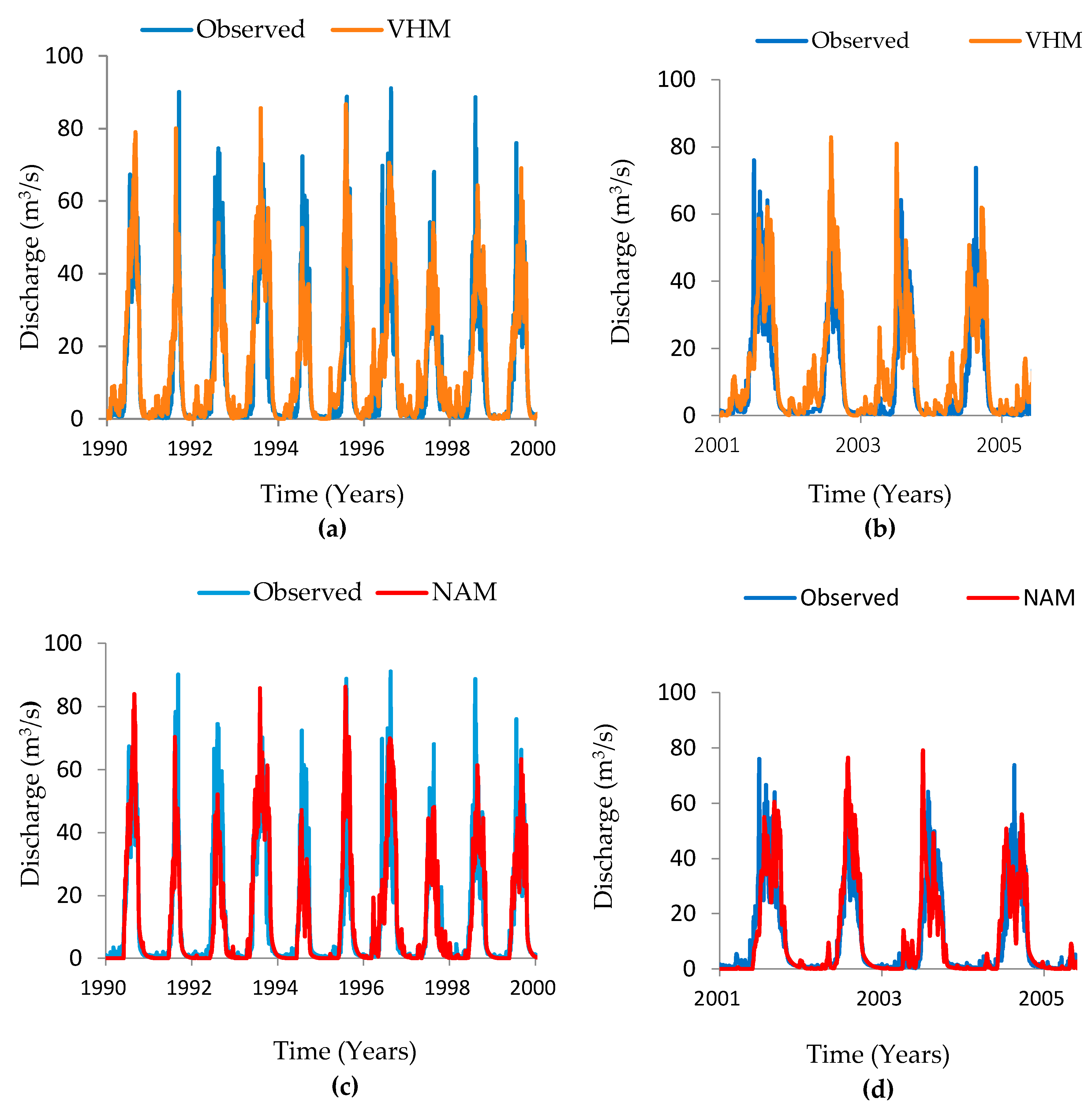
Comparison based on the graphical fitting was also made to see whether the overall shape of the hydrograph is properly captured. As seen from Figure 4, the shape of the hydrographs of the observed flow was properly captured, which indicates that the simulated flow, both by NAM and VHM, depicted a good agreement with the observed flow. However, it is noted that some of the peak flows were underestimated by the models, while the low flows were well captured.
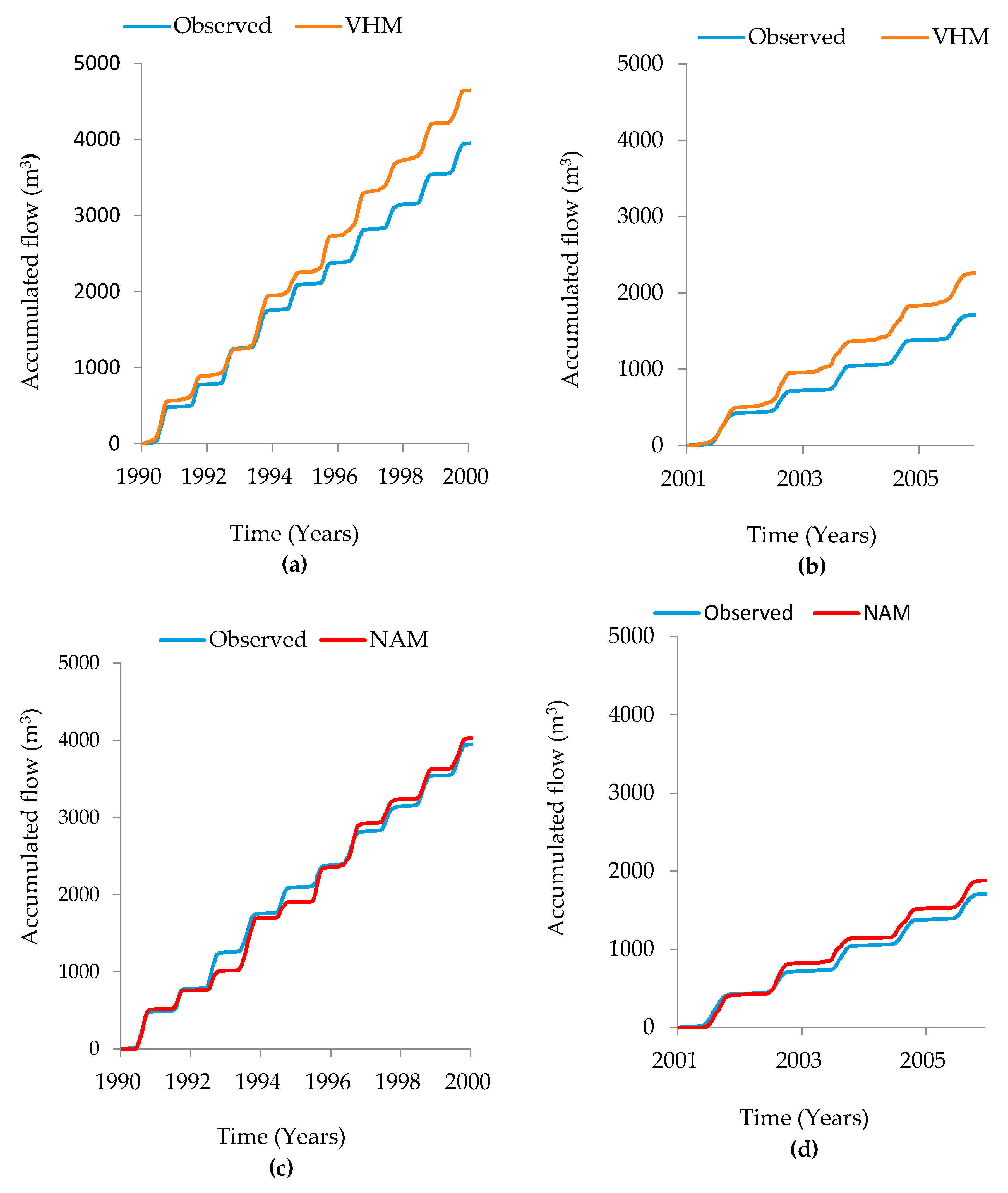
The cumulative simulated and observed flow shows a good agreement with the NAM model (Figure 5c,d) during calibration and validation periods, whereas the VHM model overestimated the cumulative flow for both periods (Figure 5a,b).
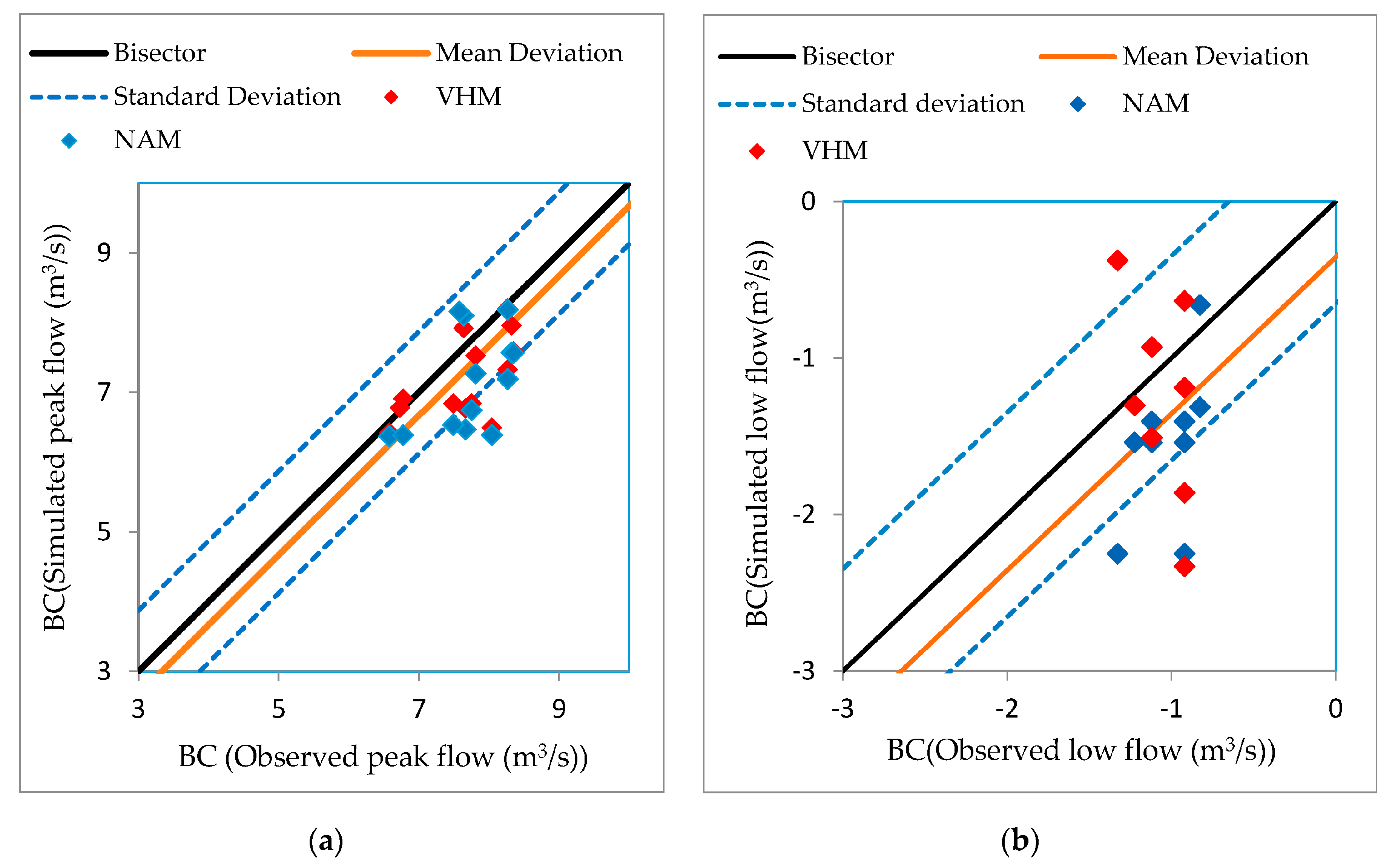
As can be observed from Figure 6a, the scatter plot of the peak flows of both models were below the mean, which specifies that the models underestimated the high flows, whereas the low flows predicted by VHM were fairly distributed along the mean line, depicting that the model is good enough at reproducing the low flow. In contrast, predicted low flows from the NAM model were below the mean line (Figure 6b).
3.3. Intercomparision of the Models
Similar performance indicators were employed for both the models, and they showed good results for the prediction of the runoff (Table 7). However, a higher difference was observed between the models in simulating the water balance (Figure 5). This might be attributed to the way they conceptualize the hydrological processes of the catchment. For instance, the VHM model relies on the proportion of the rainfall shared between the subflow components and soil moisture storage (Figure 2), whereas the NAM model depends on the soil moisture content in root zone storage (Figure 3). Thus, the overestimation of the cumulative water balance by the VHM might be attributed to the sensitivity of the model to the rainfall. Moreover, it is also noted that the two models were not able to simulate the peak flows. However, the low flow was properly captured. The models did not depict substantial differences in the description of the hydrological processes except in the simulation of the water balance. Thus, the application of multiple models for the modeling of the rainfall-runoff process increases the confidence of the use of the models as they performed equally well in the calibration and validation periods.
4. Discussion
The catchment runoff is reproduced by the models in a reasonable way. Nevertheless, the VHM depicts slightly lower performances both statistically and graphically as compared to the NAM model which might be attributed to its sensitivity to the quality of rainfall data. A similar study [19,33], conducted on Grote Nete catchment in Belgium, demonstrated the lower performances of the VHM model as compared to the NAM and PDM conceptual rainfall runoff models, which is comparable to the result obtained for this study. In addition, the HBV, VHM and NAM models were applied to predict the streamflow of the Upper Blue Nile basin at ElDiem gauge station and found that the NAM showed better performances as compared to the VHM [34]. It is clear that both the models reproduced the streamflow which was good in accordance to the observed flow. However, the overall results reflected that the NAM prediction of the streamflow was better than that of VHM. The low quality and low data availability might be possible obstacles for higher efficiency achievement in the data scarce region like the study catchment. Overall, the good agreement between the observed and simulated flow demonstrated by the two models indicates that the models can jointly allow hydrological simulation in the study catchment.
5. Conclusions
This study appraises the performances of the VHM and NAM lumped rainfall–runoff models in predicting the streamflow of a small agricultural catchment located in the southwest of the Upper Blue Nile basin. Precipitation, potential evapotransipration and discharge were used as the input to the models. The models were then calibrated for the period of 1 January 1990–31 December 2000 and validated for the period of 1 January 2001–31 December 2005. The results showed that the models predicted the flow in a good way. The shape of the hydrograph was properly simulated by the models. However, it is noted that the VHM model simulated a higher water balance compared to the NAM model. The models underestimated the high flows, while the low flows are well predicted. Intercomparision of the models based on the statistical and graphical performance indicators showed that the NAM achieved better performances than the VHM model. Generally, the two models were capable of simulating the dominant hydrological processes. However, great caution is required for application of the models in water resource management related to extreme flows.
Acknowledgments
My heartfelt thanks go to the Ethiopian Ministry of Water, Energy and Irrigation (MOWIE) and Ethiopian National Meteorological Service Agency (NMSA), for providing me with hydrometeorological data.
Conflicts of Interest
The author declares no conflict of interest.
References
- Booij, M.J.; Tollenaar, D.; van Beek, E.; Kwadijk, J.C. Simulating impacts of climate change on river discharges in the Nile basin. Phys. Chem. Earth 2011, 36, 696–709. [Google Scholar] [CrossRef]
- Taye, M.T.; Willems, P. Identifying sources of temporal variability in hydrological extremes of the upper Blue Nile basin. J. Hydrol. 2013, 499, 61–70. [Google Scholar] [CrossRef]
- Uhlenbrook, S.; Mohamed, Y.; Gragne, A.S. Analyzing catchment behavior through catchment modeling in the Gilgel Abay, upper Blue Nile River basin, Ethiopia. Hydrol. Earth Syst. Sci. 2010, 14, 2153–2165. [Google Scholar] [CrossRef]
- Tufa, D.F.; Abbulu, Y.E.; Srinivasarao, G.V. Watershed Hydrological Response to Changes in Land Use/Land Covers Patterns of River Basin: A Review. IJCSEIERD 2014, 4, 157–170. [Google Scholar]
- Gebrekristos, S.T. Understanding Catchment Processes and Hydrological Modelling in the Abay/Upper Blue Nile Basin; CRC Press: Boca Raton, FL, USA, 2015. [Google Scholar]
- Refsgaard, J.C. Terminology, Modelling Protocol And Classification of Hydrological Model Codes. In Distributed Hydrological Modelling; Abbott, M.B., Refsgaard, J.C., Eds.; Springer: Dordrecht, The Netherlands, 1996; Volume 22, pp. 17–39. ISBN 978-94-010-6599-3. [Google Scholar]
- Sandholt, I.; Rasmussen, K.; Andersen, J. A simple interpretation of the surface temperature/vegetation index space for assessment of surface moisture status. Remote Sens. Environ. 2002, 79, 213–224. [Google Scholar] [CrossRef]
- Duong, V.N.; Binh, N.Q.; Ma, Q.; Gourbesville, P. Applying Deterministic Distributed Hydrological Model for Stream Flow Data Reproduction. A Case Study of Cu De Catchment, Vietnam. Procedia Eng. 2016, 154, 1010–1017. [Google Scholar] [CrossRef]
- Vargas, R.B.; Gourbesville, P. Deterministic hydrological model for flood risk assessment of mexico city. In Advances in Hydroinformatics; Springer: Berlin, Germany, 2016; pp. 59–73. [Google Scholar]
- Andersen, J.; Refsgaard, J.C.; Jensen, K.H. Distributed hydrological modelling of the Senegal River Basin—Model construction and validation. J. Hydrol. 2001, 247, 200–214. [Google Scholar] [CrossRef]
- Carcano, E.C.; Bartolini, P.; Muselli, M.; Piroddi, L. Jordan recurrent neural network versus IHACRES in modelling daily streamflows. J. Hydrol. 2008, 362, 291–307. [Google Scholar] [CrossRef]
- Abbott, M.B.; Bathurst, J.C.; Cunge, J.A.; O’connell, P.E.; Rasmussen, J. An introduction to the European Hydrological System-Systeme Hydrologique Europeen,“SHE”, Structure of a physically-based, distributed modelling system. J. Hydrol. 1986, 87, 61–77. [Google Scholar] [CrossRef]
- Claver, A.; Wood, W. The institute of hydrology distributed model. In Computer Models of Watershed Hydrology; Singh, V.P., Ed.; Water Resources Publications: Highlands Ranch, CO, USA, 1995; pp. 595–626. [Google Scholar]
- Bergström, S. Development and Application of a Conceptual Runoff Model for Scandinavian Catchments; SMHI RHO 7; SMHI: Norrköping, Sweden, 1976. [Google Scholar]
- Burnash, R.J.; Ferral, R.L.; McGuire, R.A. A Generalised Streamflow Simulation System–Conceptual Modelling for Digital Computers; Joint Federal State River Forecasting Centre: Sacramento, CA, USA, 1973.
- Kirkby, M.J.; Beven, K.J. A physically based, variable contributing area model of basin hydrology. Hydrol. Sci. J. 1979, 24, 43–69. [Google Scholar]
- Tekleab, S.; Uhlenbrook, S.; Mohamed, Y.; Temesgen, M.; Savenije, H.H.; Wenninger, J. Water balance modeling of Upper Blue Nile catchments using a top-down approach. Hydrol. Earth Syst. Sci. 2011, 15, 2179–2193. [Google Scholar] [CrossRef]
- Onyutha, C. Influence of hydrological model selection on simulation of moderate and extreme flow events: A Case Study of the Blue Nile Basin. Adv. Meteorol. 2016. [Google Scholar] [CrossRef]
- Vansteenkiste, T.; Tavakoli, M.; Ntegeka, V.; De Smedt, F.; Batelaan, O.; Pereira, F.; Willems, P. Intercomparison of hydrological model structures and calibration approaches in climate scenario impact projections. J. Hydrol. 2014, 519, 743–755. [Google Scholar] [CrossRef]
- Jillo, A.Y.; Demissie, S.S.; Viglione, A.; Asfaw, D.H.; Sivapalan, M. Characterization of regional variability of seasonal water balance within Omo-Ghibe River Basin, Ethiopia. Hydrolog. Sci. J. 2017, 8, 1200–1215. [Google Scholar]
- Sima, B.A.; Bishop, K.; Gebrehiwot, S.G. Flow Regime and Land Cover Changes in the Didessa Sub-Basin of the Blue Nile River, South-Western Ethiopia: Combining Empirical Analysis and Community Perception. Master’s Thesis, Integrated Water Resource Management, Uppsala, Sweden, 2011. [Google Scholar]
- Haileyesus, B. Evaluation of Climate Change impacts on hydrology on selected catchments of Abbay Basin. Master’s Thesis, Addis Ababa University, Addis Ababa, Ethiopia, 2011. [Google Scholar]
- Hargreaves, G.H.; Samani, Z.A. Estimating potential evapotranspiration. J. Irrig. Drain. Div. 1982, 108, 225–230. [Google Scholar]
- Madsen, H.; Wilson, G.; Ammentorp, H.C. Comparison of different automated strategies for calibration of rainfall-runoff models. J. Hydrol. 2002, 261, 48–59. [Google Scholar] [CrossRef]
- Willems, P. Parsimonious rainfall—Runoff model construction supported by time series processing and validation of hydrological extremes—Part 1: Step-wise model-structure identification and calibration approach. J. Hydrol. 2014, 510, 578–590. [Google Scholar] [CrossRef]
- Willems, P.; Mora, D.; Vansteenkiste, T.; Taye, M.T.; Van Steenbergen, N. Parsimonious rainfall-runoff model construction supported by time series processing and validation of hydrological extremes–Part 2: Intercomparison of models and calibration approaches. J. Hydrol. 2014, 510, 591–609. [Google Scholar] [CrossRef]
- Nielsen, S.A.; Hansen, E. Numerical simulation of the rainfall-runoff process on a daily basis. Hydrol. Res. 1973, 4, 171–190. [Google Scholar]
- Danish Hydraulic Institute (DHI). DHI Mike 11: A Modelling System for Rivers and Channels, Reference Manual; DHI Water & Environment: Hørsholm, Denmark, 2011. [Google Scholar]
- Chapman, T.G. Comment on “Evaluation of automated techniques for base flow and recession analyses” by RJ Nathan and TA McMahon. Water Resour. Res. 1991, 27, 1783–1784. [Google Scholar] [CrossRef]
- Willems, P. A time series tool to support the multi-criteria performance evaluation of rainfall-runoff models. Environ. Model. Softw. 2009, 24, 311–321. [Google Scholar] [CrossRef]
- Nash, J.E.; Sutcliffe, J.V. River flow forecasting through conceptual models part I—A discussion of principles. J. Hydrol. 1970, 10, 282–290. [Google Scholar] [CrossRef]
- Box, G.E.; Cox, D.R. An analysis of transformations. J. R. Stat. Soc. 1964, 26, 211–243. [Google Scholar]
- Vansteenkiste, T.; Pereira, F.; Willems, P.; Mostaert, F. Effect of Climate Change on the Hydrological Regime of Navigable Water Courses in Belgium: Subreport 2—Climate Change Impact Analysis by Conceptual Models; WL Rapporten; Waterbouwkundig Laboratorium: Antwerpen, Belgium, 2012. [Google Scholar]
- Onyutha, C.; Willems, P. Identification of the main attribute of river flow temporal variations in the Nile Basin. Hydrol. Earth Syst. Sci. Discuss. 2015, 12, 12167–12214. [Google Scholar] [CrossRef]
Figure 1.
The Upper Guder catchment.
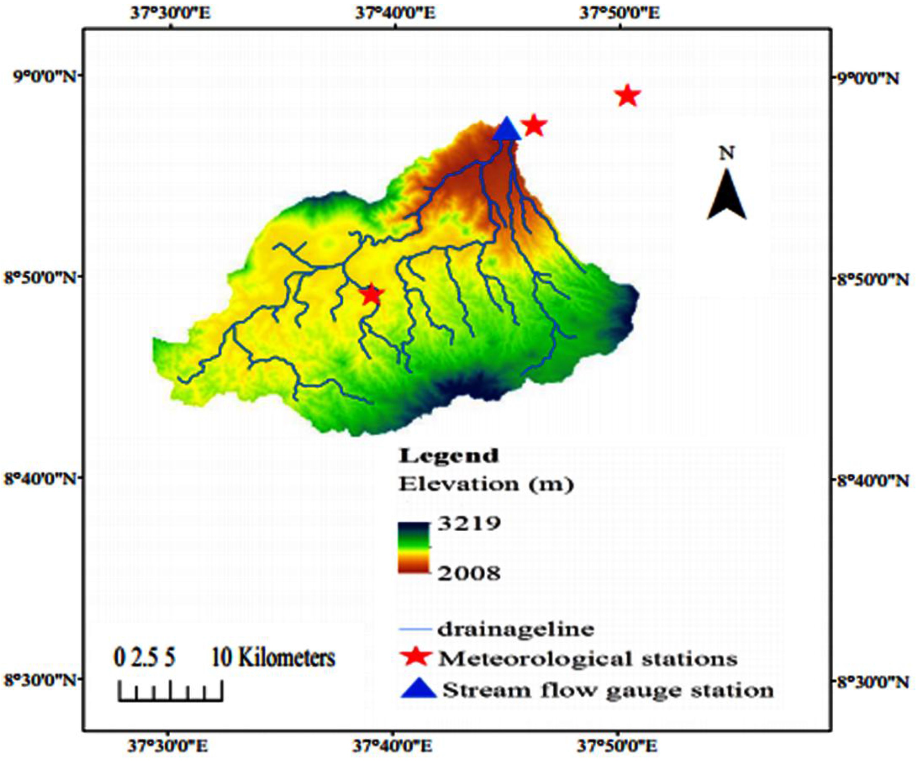
Figure 2.
Model structure of the Veralgemeend Conceptueel Hydrologisch model.
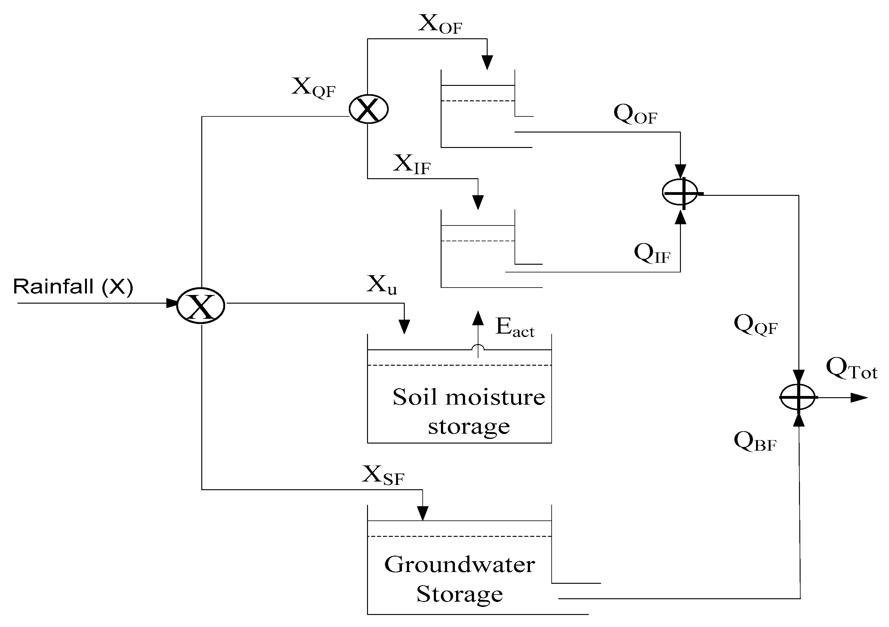
Figure 3.
Model structure NedborAfstromnings Model.
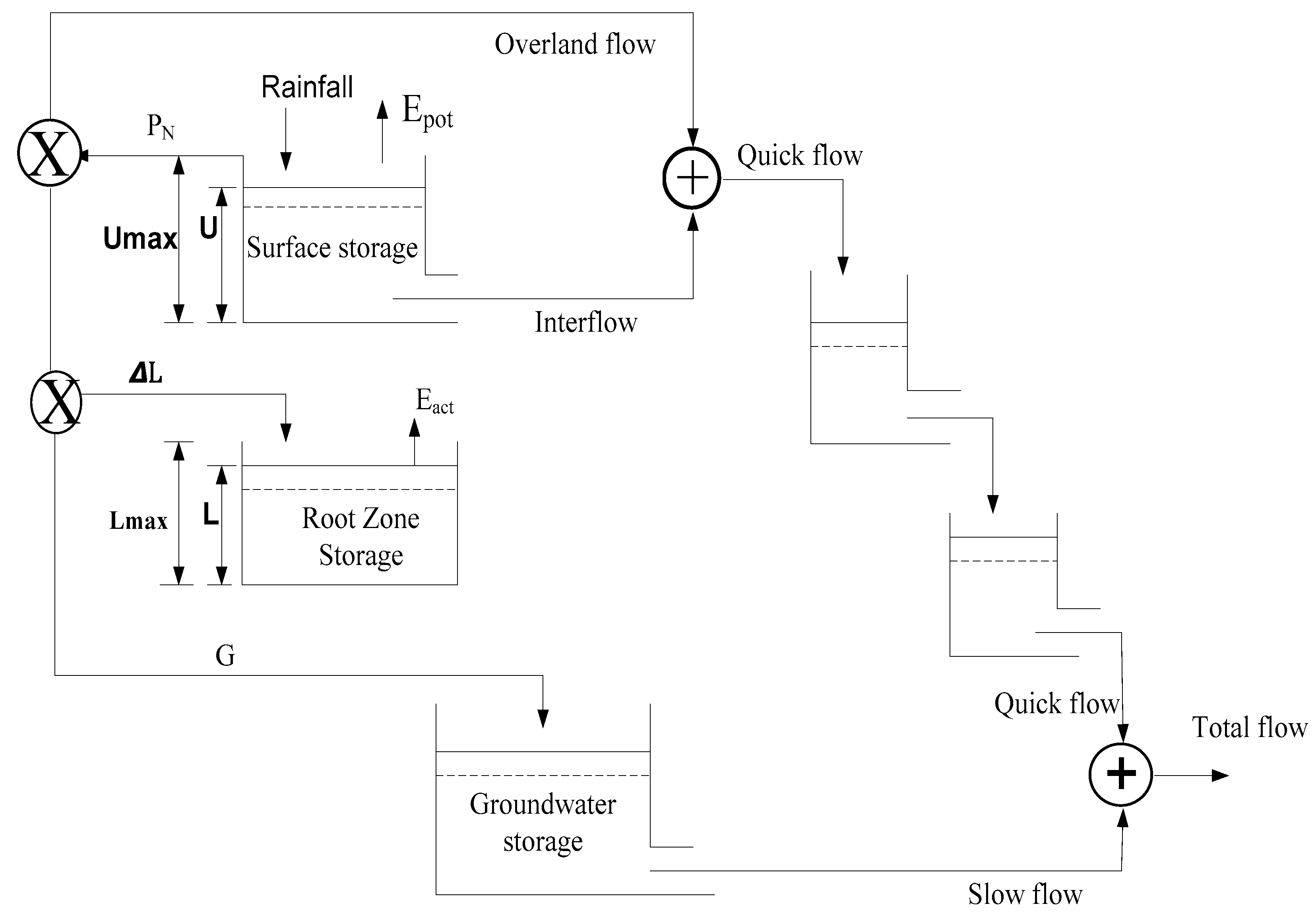
Figure 4.
Observed and simulated flow for calibration and validation period: (a,b) for VHM, and (c,d) for the NAM.
Figure 4.
Observed and simulated flow for calibration and validation period: (a,b) for VHM, and (c,d) for the NAM.

Figure 5.
Cumulative observed and simulated flow for calibration and validation period: (a,b) for VHM, and (c,d) for the NAM.
Figure 5.
Cumulative observed and simulated flow for calibration and validation period: (a,b) for VHM, and (c,d) for the NAM.

Figure 6.
The scatter plot of simulated and observed: (a) peak flow and (b) low flow.


Table 1.
Characteristics of data.
| Data | Unit | Source | Length of Record |
|---|---|---|---|
| Rainfall | mm | NMSA | 1990–2005 |
| Temperature | °C | NMSA | 1990–2005 |
| PET | mm | Calculated | 1990–2005 |
| Discharge | m3/s | MOWIE | 1990–2005 |
NMSA: National Meteorological Service Agency; MOWIE: Ministry of Water, Irrigation and Energy in Ethiopia; PET: potential evapotransipration.
Table 2.
Parameters and variables of the VHM model.
| Parameters Description | Parameters |
|---|---|
| Initial soil water content | Uini (mm) |
| Maximum soil water content | Umax (mm) |
| Soil water content at maximum evapotranspiration | Uevap (mm) |
| Baseflow submodel | |
| Baseflow separation process parameters | c1 (-), c2 (-), c3(-) |
| Overland flow submodel | |
| Surface runoff separation process parameters | c1 (-), c2 (-), c3 (-), c4 (-) |
| Interflow submodel | |
| Interflow separation process parameters | c1 (-), c2 (-), c3 (-), c4 (-) |
| Recession constant for slow flow | KSF (days) |
| Recession constant for Interflow | KIF (days) |
| Recession constant for overland flow | KOF (days) |
| Variable Description | Variables |
| Rainfall fraction shared as quick flow | XQF (mm) |
| Rainfall fraction shared as slow flow | XSF (mm) |
| Rainfall fraction shared as storage flow | Xu (mm) |
| Rainfall fraction shared as overland flow | XOF (mm) |
| Rainfall fraction shared as interflow | XIF (mm) |
| Actual evapotransiparation | Eact (mm) |
| Total discharge | QTot (m3/s) |
| Quick flow | QQF (m3/s) |
| Interflow | QIF (m3/s) |
| Overland flow | QOF (m3/s) |
| Base flow | QBF (m3/s) |
| Antecedent rainfall | r (mm) |
Table 3.
Parameters and variables of the NedborAfstromnings (NAM) model.
| Parameter Descriptions | Parameter | Variable Descriptions | Variable |
|---|---|---|---|
| Maximum water content in surface storage | Umax (mm) | Surface storage water content | U (mm) |
| Maximum water content in lower zone storage | Lmax (mm) | Lower storage soil water content | L (mm) |
| Overland flow runoff coefficient | CQOF (-) | Actual evapotranspiration | Eact (mm) |
| Time constant in the interflow | CKIF (h) | Potentail Evapotransipration | Epot (mm) |
| Time constant for overland and interflow flow | CK1,2 (h) | Inflitration to root zone | ΔL (mm) |
| Threshold value for interflow | TIF (-) | Groundwater recharge | G (mm) |
| Threshold value for overland flow | TOF (-) | Excess rainfall | PN (mm) |
| Time constant for baseflow | CKBF (h) | ||
| Threshold value for ground water storage | TG (-) |
Table 4.
The recession constant and w-factor of the stream flow.
| Parameter | Overland Flow | Interflow | Baseflow |
|---|---|---|---|
| K (days) | 1 | 6 | 36 |
| w (-) | 0.14 | 0.10 | 0.76 |
Table 5.
Calibrated set of parameters for the VHM model.
| Baseflow Submodel | Overland Submodel | Interflow Submodel | Routing Submodel | ||||
|---|---|---|---|---|---|---|---|
| Umax | 250 | c1 | −3.55 | c1 | −1.83 | KBF | 40 |
| Uevap | 80 | c2 | 1.45 | c2 | 1.20 | KIF | 5 |
| Uini | 40 | c3 | −1 | c3 | −0.5 | KOF | 1 |
| c1 | 1.74 | c4 | 0.5 | c4 | 0.2 | ||
| c2 | 0.15 | λ | 1 | λ | 1 | ||
| c3 | 1.19 | r | 0.1 | r | 0.1 | ||
Table 6.
Calibrated set of parameters for the NAM model.
| Parameter | Umax | Lmax | CQOF | CKIF | CK1,2 | TIF | TOF | CKBF | TG |
|---|---|---|---|---|---|---|---|---|---|
| Calibrated Value | 30 | 220 | 0.25 | 150 | 35 | 0.2 | 0.1 | 850 | 0.25 |
Table 7.
Statistical performance of the models.
| Calibration | Validation | |||
|---|---|---|---|---|
| VHM | NAM | VHM | NAM | |
| NSE (-) | 0.67 | 0.71 | 0.58 | 0.60 |
| WBD (%) | −13.7 | −0.1 | −17 | −9 |
| R2 (-) | 0.70 | 0.73 | 0.66 | 0.69 |
© 2017 by the author. Licensee MDPI, Basel, Switzerland. This article is an open access article distributed under the terms and conditions of the Creative Commons Attribution (CC BY) license (http://creativecommons.org/licenses/by/4.0/).
Share and Cite
MDPI and ACS Style
Wakigari, S.A. Evaluation of Conceptual Hydrological Models in Data Scarce Region of the Upper Blue Nile Basin: Case of the Upper Guder Catchment. Hydrology 2017, 4, 59. https://doi.org/10.3390/hydrology4040059
AMA Style
Wakigari SA. Evaluation of Conceptual Hydrological Models in Data Scarce Region of the Upper Blue Nile Basin: Case of the Upper Guder Catchment. Hydrology. 2017; 4(4):59. https://doi.org/10.3390/hydrology4040059
Chicago/Turabian StyleWakigari, Shimelis Asfaw. 2017. "Evaluation of Conceptual Hydrological Models in Data Scarce Region of the Upper Blue Nile Basin: Case of the Upper Guder Catchment" Hydrology 4, no. 4: 59. https://doi.org/10.3390/hydrology4040059
Note that from the first issue of 2016, this journal uses article numbers instead of page numbers. See further details here.