On Rigorous Drought Assessment Using Daily Time Scale: Non-Stationary Frequency Analyses, Revisited Concepts, and a New Method to Yield Non-Parametric Indices


Faculty of Technoscience, Muni University, P.O. Box 725, Arua, Uganda
Hydrology 2017, 4(4), 48; https://doi.org/10.3390/hydrology4040048
Submission received: 15 September 2017
/
Revised: 24 October 2017
/
Accepted: 25 October 2017
/
Published: 29 October 2017
Abstract
:Some of the problems in drought assessments are that: analyses tend to focus on coarse temporal scales, many of the methods yield skewed indices, a few terminologies are ambiguously used, and analyses comprise an implicit assumption that the observations come from a stationary process. To solve these problems, this paper introduces non-stationary frequency analyses of quantiles. How to use non-parametric rescaling to obtain robust indices that are not (or minimally) skewed is also introduced. To avoid ambiguity, some concepts on, e.g., incidence, extremity, etc., were revisited through shift from monthly to daily time scale. Demonstrations on the introduced methods were made using daily flow and precipitation insufficiency (precipitation minus potential evapotranspiration) from the Blue Nile basin in Africa. Results show that, when a significant trend exists in extreme events, stationarity-based quantiles can be far different from those when non-stationarity is considered. The introduced non-parametric indices were found to closely agree with the well-known standardized precipitation evapotranspiration indices in many aspects but skewness. Apart from revisiting some concepts, the advantages of the use of fine instead of coarse time scales in drought assessment were given. The links for obtaining freely downloadable tools on how to implement the introduced methods were provided.
1. Introduction
For a particular region, the sustained condition of the water availability being below a certain threshold characterizes drought [1]. Drought leads to negative impacts, which can be social, economical, etc. [2]. For effective monitoring of drought, detailed representation of the information on drought severity, spatial extent, and impacts may be required [3]. For hydrological drought, frequency analyses can be conducted using river flow. For meteorological drought, precipitation tends to be used. However, for a reasonable representation of the meteorological drought with respect to water balance, as will be seen implemented in this paper, the difference between precipitation and evaporation can be used. Some of the methods for analyses of drought include the crop moisture index [4], Standardized Precipitation Index (SPI) [5], standardized groundwater level index [6], Standardized Precipitation Evapotranspiration Index (SPEI) [7], Palmer drought severity index [8], etc. Most of (if not all) these existing drought analyses methods make use of coarse (e.g., monthly or annual) time scales.
The main problem of the SPI and other related methods is that they tend to yield skewed indices. Furthermore, the indices from these methods have no clear bounds. To capture the data skewness, some distributions must be assumed and followed by approximate transformations, e.g., that provided by Abramowitz and Stegun [9] to obtain the indices. Gamma distribution is commonly used for the SPI, while, for SPEI, the Log-logistic distribution was proposed by Vicente-Serrano et al. [7]. However, Stagge et al. [10,11] recommended the generalized extreme value distribution instead of the Log-logistic distribution for SPEI. The recently sparked debate on the proposal and recommendation about which distribution to use for SPEI is not trivial (see [10,11,12]). It remains apparent that the uncertainty in the parameter estimation of the non-Gaussian distributions further compounds the unreliability of the skewed indicators of hydro-meteorological conditions.
For frequency analysis, fine temporal resolution of the hydro-climatic data, e.g., flow or rainfall, is required. When it comes to frequency analysis in hydrometeorology, the use of high resolution data, e.g., daily flow or rainfall, tends to be geared more considerably towards the analyses of flood than dry conditions. This could be because high peak flow results in an immediate surplus of water, which can be disastrous to lives and property. On the other hand, drought results from a progressive insufficiency of water, the effects of which are not immediate from the drought onset; thus, the use of temporally coarse data for the common methods for drought analyses. However, the conventional use of coarse (e.g., monthly or annual) time scale in which the data are averaged in a non-overlapping way leads to: (i) lack of insight on how to explain the aggregated variation from the coarse temporal scale; (ii) reduced flexibility to combine possible drought attributes of high temporal resolution to yield relevant drought information in a statistically compressed way; and (iii) lack of relevant information, especially on drought onset if required in number of days or weeks , etc. Recently, Sawada et al. [13] developed an eco-hydrological model for application to drought analysis at a basin-wide scale. To improve drought identification, the authors attempted to address the importance of introducing dynamic vegetation modeling within a distributed hydrological model. Although Sawada et al. [13] used daily time series for modeling, in the analyses of drought indices, they still made use of the conventional monthly time scale. The advantages of the use of fine instead of the conventional coarse time scales in drought assessment can be found in Appendix C of this paper.
Furthermore, drought analyses tend to be commonly conducted considering stationarity. It is possible that the hydro-meteorological extreme events can be characterized by a possible deterministic function of time. Return levels estimated through the assumption of stationarity can be far different from those obtained when non-stationarity is analogously considered. Some of the recent studies that considered non-stationarity analyses of drought include [14,15]. Cancelliere [14] gave a brief review of approaches for modeling non-stationary time series with an extension to model drought length, while Wang et al. [15] proposed a time-dependent SPI. However, similar to other past studies on drought analyses, both Cancelliere [14] and Wang et al. [15] followed the use of coarse time scale.
The main gaps in drought assessment that this paper intended to address are as follow: analyses tend to focus on coarse temporal scales, many of the existing methods yield skewed indices, a few terminologies are used ambiguously, and analyses comprise an implicit assumption that the observations come from a stationary process. Solutions to the above problems in this paper were by: introducing non-stationary frequency analyses of extreme events, revisiting some concepts on, e.g., incidence, extremity, etc. (to avoid ambiguity in the use of certain key terms based on daily time scale) through shift from monthly to daily time scale, introducing an approach on how to use non-parametric rescaling to obtain robust indices which are not (or minimally) skewed, and demonstrating the advantages of the use of daily instead of monthly time scales. With respect to the introduced non-stationary frequency analyses, the new method makes use of either the significance of the trend or statistical simulation of extreme events constrained to the obtained trend magnitude. As will be found in Section 2.2.1, to conduct trend analyses for the proposed non-stationary frequency analyses, the author makes use of both old and recently introduced methods. By the time of conducting this study, the methods introduced in this paper were never used before for drought analyses. For hydrological and meteorological drought, the proposed method makes use of river flow and precipitation insufficiency (i.e., precipitation minus potential evapotranspiration), respectively.
It is a common practice to compare results from a new method with those from existing approaches for drought analyses (see, e.g., [16,17]); this is because of the differences among the various methods in capturing different aspects of drought. Eventually, in this paper, comparison was made between results from data of daily and monthly temporal resolutions. Differences between conventional methods and the new methods introduced in this paper were also elaborately tackled. Illustrations on why the use of daily time series should be preferred to monthly data were given.
2. Methods
2.1. Data for the Case Study
For illustration of the non-stationary frequency analysis of drought, daily rainfall intensity, potential evapotranspiration (ET0) rate and river flow data from the Blue Nile basin of Ethiopia and Sudan in Africa were used. The Blue Nile basin (Figure 1) has a catchment area of about 325,000 km2. The Blue Nile, which emanates from the Ethiopian Highlands based on the two main tributaries, the Dinder and Rahad Rivers, flows into and out of Lake Tana. The climate of the basin is characterized by seasonal migration of the inter-tropical convergence zone. According to the International Water Management Institute IWMI [18], the majority of the population where the Blue Nile basin is located depends on rain-fed cropping system to support livelihoods.
Daily river flow recorded at Khartoum from 1965 to 2002 was adopted from a previous study [19] conducted by the author of this paper regarding the influence of hydrological model selection on simulation of moderate and extreme flow events. The flow data after 2002 were not available for analyses, although they would be vital to obtain an insight into the effects of recent variability on hydrology of the Blue Nile basin. Climate Forecast System Reanalysis (CFSR) high-resolution gridded (0.3° × 0.3°) daily meteorological data including rainfall (mm/day), solar radiation (Srad, MJ/m2/day) as well as the minimum (Tmin, °C) and maximum (Tmax, °C) temperature were obtained from the National Centers for Environmental Prediction NCEP [20] database. These meteorological time series which were from 1979 to 2000 were extracted over the region covering latitude from 5° to 17° N and longitude from 30° to 42° E. Based on the Srad, Tmin and Tmax, ET0 (mm/day) was computed at each grid point using the Food and Agriculture Organization (FAO)-Penman-Monteith method [21]. At each grid point, the daily precipitation insufficiency was computed by subtracting the ET0 from precipitation.
To construct Thiessen polygon [22] for obtaining catchment-wide averaged precipitation insufficiency, rainfall stations were required. From the meteorological stations, only their locations were used to construct the Thiessen polygon. To obtain basin-wide averaged precipitation insufficiency, data over the period 1979–2000 from the CFSR were used. For an overview of the spatial difference in long-term rainfall statistics across the basin, daily rainfall observed at nine meteorological stations (see Table 1 and Figure 1) were obtained from the global historical climatology network [23]. It is noticeable that the long-term coefficient of variation (CV) (in terms of the ratio of the standard deviation to the mean) varied from 1.94 (Station 4) to 8.31 (Station 7). This shows that the study area had, over the data period, considerable amount of day-to-day variability in rainfall. The coefficient of skewness in the last column of Table 1 shows that the daily rainfall time series over the data period were positively skewed, and thus, not of the Gaussian distribution.
2.2. Stationarity versus Non-Stationarity
For clarity, in this paper, stationarity is the time-invariance of statistical properties of the variable being considered for analyses. One example of such statistical properties especially for drought categorization is the ratio of the difference between the variable and the long-term mean to the standard deviation of the variable. If the statistical properties of the variable depend on time of the observations, the series can be assumed to come from a non-stationary process. However, for frequency analyses of extreme events, stationarity can be characterized by time-invariance of the extreme value distribution properties. For non-stationarity process, there should exist a deterministic function of time [24]. For the introduced method, the considered function of time is the linear trend. The introduced methodology (described hereafter) is implemented in a freely available tool for Frequency Analyses considering Non-stationarity (FAN-Stat), which can be downloaded via https://sites.google.com/site/conyutha/tools-to-download (accessed: 14 September 2017).
There are some basic requirements for analyzing the frequency of events.
2.2.1. Pre-Requisites for Frequency Analysis
Data Transformation
Considering hydrological drought, for the ease of extreme value analysis of low flow in a similar way as that for high flow, the given discharge or river flow time series H can be transformed by (1/H). This is because the use of (1/H) makes the low flows to follow the generalized Pareto distribution or exponential instead of Weibull or Fréchet distribution as clearly shown by Onyutha [19]. In other words, the (1/H) transformation simplifies drought frequency analyses to be conducted in a way analogous to that for obtaining flood quantile estimates. What cannot escape a quick notice is that the (1/H) transformation is possible for non-ephemeral rivers (i.e., for H > 0). Of course, if the flow time series are characterized by zeros, a different consideration instead of (1/H) transformation may be adopted. For instance, the frequency of hydrological dry spells can be analyzed so long as they can be extracted in a way to ensure their independency.
For frequency analysis of meteorological drought, again, it is vital for the precipitation insufficiency to be transformed by negation i.e., −1 × H. This makes the negative values positive and vice versa thereby simplifying the extraction of the independent events and the subsequent extreme value analysis. The (−H) transformation is used instead of the (1/H) to avoid exaggeration since some of the deficits (especially those during dry season) can be already small and negative.
Independence of the Extreme Events
For quantile estimation, the extreme events are required to be independent and identically distributed. To extract the extreme events from the full time series, Peak Over Threshold (POT) approach (see, e.g., [25,26]) or the Annual Maxima Method (AMM) (see, e.g., [27]) can be used. For the AMM, the maximum event in each hydrological year is extracted. The AMM yields events with strong independence. However, the number of the extreme events tends be limited especially for data of short record length. To generate an adequate number of events to provide a reasonable definition of extreme value region, the POT method is often preferred to the AMM approach. Extraction of independent extreme events can be done using the method of POT based on the independence criteria. In this study, the independence criteria, based on daily time scale, used were as follow:
- (i)
- the time in between the two events should not be less than the stipulated value;
- (ii)
- the extracted event should not be less than the specified threshold; and
- (iii)
- the independency ratio should not be greater than a stipulated value.
Independency ratio, with respect to the two events within the time slice under consideration, refers to the small value divided by the large one. The threshold can be specified as a percentage of the maximum event in the time series. The independency ratio can also be specified in percentage. The number of the extracted POTs depends on the sensitivity of each of the parameters defining the independency of the events. It can be expected that the lower (higher) the threshold, the larger (smaller) the number of POT events. The smaller (larger) the independency ratio, the fewer (larger is the number of) the POT events. The larger the inter-event time, the more likely the strong independence of the POTs will be. The independence criteria were modified in this study following the information from [26,28]. As a side note, both the POT events, and their corresponding or the Required Times of Observation (RTO) should be extracted. The detail on how to obtain the RTOs can be found from Section 1.1.b of the Supplementary Materials.
For ephemeral rivers (i.e., those which dry up over some periods), hydrological dry spell or deficit period can be analyzed instead of low flow events. A hydrological dry day is defined as the day with daily flow below a certain flow threshold. Hydrological dry spell (in days) refers to period when the number of consecutive days with hydrological deficit is greater than a stipulated threshold. In this study, for illustration, the daily flow threshold was set to 800 m3/s. The minimum number of days to characterize a hydrological dry spell was set to 175 days.
The number of the POT events depends on the set of parameters used to characterize the independency criteria. For instance, if the other independency criteria (i.e., inter-event time and independency ratio) for the extraction of extreme events are kept constant, by increasing the threshold, the number of extreme events is expected to increase. The magnitude (and, if possible, the directional sign) of the trend may also change when the threshold is increased or reduced. The bottom line is that the POTs should be extracted independent of time such that the number of the extreme events is adequate enough to characterize more consistent definition of the extreme value region than for the case when the annual maxima model is used.
Significance of Trend in the Data
A trend comprises both the magnitude and direction. Trend direction shows whether the dependence of the variable on time is in a positive (i.e., increasing) or negative (i.e., decreasing) way. Trend magnitude expresses the amount by which the variable is expected to linearly change over a time unit of the observations. The presence of possible outliers in the data may influence the trend magnitude if detected using least squares approach. In other words, the least squares method, although is fast and simple for computation, yields a biased estimate of the trend slope. Furthermore, the presence of an outlier can also affect the standard deviation of the observations, and correlation coefficient, which are all used for the computation the standard error of estimate (see Section 1.1.c of the Supplementary Materials). Trend direction can be determined using non-parametric trend tests. The trend direction detected through a non-parametric test is not (or minimally, if possible) influenced by the presence of an outlier. This is because, the data values are replaced by their ranks, and thus, the effect of outliers on the trend direction is eliminated or tremendously reduced. However, trend direction can be influenced, e.g., by the noise. The noise in the data influences the sample variation which can be thought of in terms of the CV. The higher CV, the less powerful is the trend test [29,30]. It becomes possible that, even for a very small magnitude of linear trend (which may not be that important in practice), the null hypothesis H0 (no trend) can be rejected using trend direction [30,31]. Conversely, the H0 (no trend) cannot be rejected for a linear trend whose slope or magnitude is so huge that it may not be disregarded for decision making on the planning and management of water resources [30,31]. Therefore, there is need to assess the significance of both trend magnitude and direction before extreme value analysis of hydrological extremes, especially if non-stationarity is to be considered.
(i) Trend magnitude
Trend magnitude can be computed in terms of the linear slope m using [32,33]
where xj and xi are the jth and ith observations, respectively. Because the RTOs of the POTs can be unevenly spaced, the denominator (j − i) of Equation (1) should be replaced by their corresponding jth and ith RTOs, respectively. However, for the annual maxima time series, Equation (1) can be used as it is i.e., using the actual j and i values since the years of observations remain evenly spaced.
To assess the significance of the computed m from Equation (1), the steps based on the least squares approach as clearly presented following the author's own previous work [34] (see Section 1.1.c of the Supplementary Materials) can be used.
(ii) Trend direction
Trend direction can be assessed in terms of the significance of the non-zero slope of a linear variation in the extreme events. This can be done by testing the H0 (no trend) at the selected significance level αs%. Several non-parametric methods exist for trend detection including the Mann–Kendall (MK) [35,36], Spearman’s Rho (SMR) [37,38,39], and Cumulative Sum of rank Difference (CSD) [30,34,40] tests. The CSD trend test was recently developed by the author of this paper and applied to assess changes in the hydrometeorology of the River Nile basin. It is well-known that the MK and SMR tests rely purely on statistical results. However, the use of purely statistical trend results might be meaningless sometimes [41]. Eventually, the CSD makes use of both graphical diagnoses and statistical analyses. The graphical component of the CSD test is based on the pattern of the partial terms of the trend statistic that eventually are statistically used to test the H0 (no trend) in the data [30,34,40]. When data have no ties and are not auto-correlated, the trend detection methods are comparable in performance for various circumstances of sample size, variation, slope, etc., as shown by Yue et al. [29] for MK and SMR, and Onyutha [30] for CSD and MK. However, the differences among these methods are not negligible when applied to detect trends in time series with persistent fluctuations [34]. In trend analyses, the use of one method leads to uncertainty in the results due to the influence from the choice of the method [34,42]. Therefore, CSD and MK tests were adopted in this paper.
Let the given data be represented by X. Another time series Y can be obtained as the replica of X. The rescaled time series c in terms of the exceedance and non-exceedance counts of data points can be obtained by Onyutha [30]:
Where
and the trend statistic TCSD is computed using Onyutha [30]:
A positive/negative value of TCSD indicates an upward/downward linear trend. The distribution of TCSD is approximately normal with the mean of zero and variance (V1) given by Onyutha [34,40]:
where b is the measure of ties in the data such that
and sgn2(yj − xi) is as defined in Equation (4).
Consider Zαs/2 as the standard normal variate at αs%, while ZCSD denotes the standardized trend statistic which follows the standard normal distribution with mean of zero and the variance equals to one. If |ZCSD| ≥ |Zαs/2|, the H0 (no trend) is rejected at αs%, otherwise the H0 is not rejected at the αs%. Generally, the ZCSD can be computed using
where, according to Onyutha [40],
and, is the lag-k serial coefficient (significant at αs%). The can be computed using detrended time series Q obtained by Qi = Xi − m × i based on m from Equation (1). Considering Q# as the mean of Qi, the values of the rk can be computed using [43]:
and the (100 − αs)% confidence intervals limits (CL) for testing the significance of the rk can be computed using Anderson [44]:
and in both Equations (10) and (11), k should be set to vary from k = 1 up to n − 2 (see Onyutha [40]).
Further information on the suitability of the CSD trend statistic variance correction considering various persistence models can be found in Appendix A. To observe changes in a visual way, the CSD makes use of the plot of the cumulative sum of ci from Equation (2) versus the time of observation (for details, see Appendix B). To implement the CSD trend test, a freely downloadable tool CSD-NAIM can be obtained from https://sites.google.com/site/conyutha/tools-to-download (accessed on: 14 September 2017).
Given that the MK test is well-known, the description of its procedure for trend detection was not included in this paper but can be found in Section 1.1.c of the Supplementary Materials.
(iv) Decision to adopt stationarity or non-stationarity for frequency analyses of extreme events
Given the results of trend analyses, decision can be made on whether to analyze the frequency of extreme events considering non-stationarity. The guide for such a decision is summarized in Table 2 the use of which can be based on long-term data, say, record length of 30 years and above. For a general application, prudence should be exercised in the interpretation of the information from Table 2. First and foremost, for drought frequency analyses, the significance of both trend direction and trend magnitude should be determined using transformed data, i.e., (1/H) flow or (−H) precipitation insufficiency. Secondly, there should be more concern for a decreasing than an increasing trend in the extreme low events. In other words, concern to consider non-stationarity should be based on m > 0 for (1/H) flow or (−H) precipitation insufficiency. Of course, after back-transformation of the data, the positive m becomes negative for (H) flow or (H) precipitation insufficiency and vice versa. While analyzing dry spells, there should be more concern for an increase than a decrease in the dry spells; in other words, m > 0 can be taken into perspective when dealing with drought assessment.
2.2.2. Frequency Analyses of Stationary Extremes
Extreme value distribution can be fitted to the extracted independent extreme events. It is known that the POT events follow the Generalized Pareto Distribution (GPD) [45] (see Equations (12) and (13)). The GPD is valid for values of h above the threshold ht such that:
where G(h) is the cumulative distribution function of the GPD with scale (α), shape (γ) and location or threshold (ht) parameters.
The GPD is classified as normal, heavy and light tailed when γ = 0, γ > 0 and γ < 0, respectively. Quantile plots can be used to visually identify the classes of the GPD. Normally, hydro-meteorological variables (e.g., rainfall and ET0 do not show upper limits), and therefore, the heavy and normal-tailed cases are more common than the light-tailed GPD distribution. To identify the case γ > 0, Pareto quantile plot (i.e., (−ln{1 − G(h)}) in abscissa versus the ln(h) in ordinate) can be used. In the Pareto quantile plot, the heavy-tailed GPD (Equation (12)) appears as a straight line. Eventually, the γ (which approximates to the slope of straight line) can be computed by the least square weighted linear regression technique (Equation (14)), and for the case of γ ≠ 0, the parameter α = γ × ht. To identify the normal-tailed (or exponential) case (i.e., γ = 0) of the GPD, the exponential quantile plot i.e.; (−ln{1 − G(h)}) in the abscissa is plotted against h as the ordinate. The GPD class with γ = 0 appears as a straight line in the exponential quantile plot. It is self explanatory why a straight line is expected in the quantile plot. In fact, using Equation (13), −ln{1 − G(h)} = (h − ht)/α implying a straight line with the slope (1/α) and intercept (−ht/α). Eventually, when γ = 0, the parameter α can be computed using Equation (15) based on the weighting factor proposed by Hill [46] constrained to t number of events above ht.
For both the normal and heavy tailed cases of the GPD, instead of (−ln{1 − G(h)}), the quantile function which is also sometimes called the reduced variate {−ln(i/(n′ + 1))} can be used for the horizontal axis, where, i = 1, 2, ..., n′ and n′ denote the sample size of the POT events. The theoretical quantile of an empirical quantile hi for i = 1, 2, ..., n′ is defined in terms of the inverse distribution G−1(1 − ai) where ai = i/(n′ + 1) and corresponds to the Weibull plotting position of a quantile plot. The simplest function that is independent of the parameter values of G(h) but instead linearly depends on G−1(1 − ai) is called a quantile function M(a). Thus, M(a) = −ln(a) = −ln{1 − G(h)}. This is the basis upon which the plot of empirical versus theoretical quantiles (also called quantile-quantile plot) can be used to visualize the tail shape of the particular class of the GPD.
The optimal ht is the h above which the extreme value distribution fitted to the t observations yields the minimum average bias. In the calibration procedure, for every selected value t, how well the fitted extreme value distribution appears in the tail of the distribution can be visually checked and confirmed through statistical computation of average bias, e.g., of the theoretical from empirical return periods.
In the next step, an empirical return period T (in years) is computed as the ratio of the data record length w (in years) to the rank j of the extreme events (ordered such that j = 1 is for the highest ranking value). Theoretically (especially for making extrapolations, i.e., estimating quantiles of T larger than w), the T (in years) can be computed using Equation (16) where RT is theoretical quantile corresponding to a selected T.
To characterize severity of a drought quantile, the RT can be computed using Equations (17) and (18).
Finally, the computed RT should be back-transformed using (1/H) and (-H) when analysis is being done using low flow events and precipitation insufficiency, respectively.
2.2.3. Frequency Analyses of Non-Stationary Extremes
Non-stationary frequency analyses can be implemented in two ways.
This method is simple to implement and fast in computation. It requires the specification of significance level αs% to obtain a scaling factor Ω for modifying the observed extreme events. The αs% can be specified based on its relevance for the intended application or the expert judgment of the practitioner. Normally, αs = 5% is commonly used for hydro-meteorological research. Alternatively, the significance of the trend slope can be used. Thus, the αs% can be taken as the p-value (probability value) computed based on the trend magnitude. To compute Ω, rank the extracted POT events of size n′ from the highest to the lowest and select λ as the ({0.005 × αs%} × n′)th highest value. Next, the scaling factor is computed using Ω = λ − ht where ht is as defined in Equations (12) and (13). The quantile
Method 1: The use of significance of quantiles
can be computed using where RT is obtained using Equation (17) or (18) depending on the shape parameter γ.Method 2: The use of statistical simulation of extreme events
The following step-wise procedure can be adopted for this approach.
- (1)
- Obtain the plot of POTs versus the RTOs and compute the intercept of the linear trend line.
- (2)
- Detrend the POTs to obtain Qi = POTi − (m × RTOi + intercept) for i = 1, 2, ..., n′. Obtain Qmin i.e., the absolute value of the minimum residual time series Qi using Qmin = |min(Qi)|.
- (3)
- Investigate which correlation model the extreme events follow. The persistence model can be used for generating the synthetic extreme events. Assuming that the remaining persistence in the POTs following the application of the independence criteria for extracting the extreme events is of the lag-1 autoregressive AR(1) process, compute the AR(1) serial correlation coefficient r1 of the detrended time series Qi using Equation (10). The AR(1) was assumed for illustration purpose. Persistence may be of the forms characterized by the fractional Gaussian noise, fractionally integrated autoregressive moving average, autoregressive integrated moving average, discrete fractional Brownian motion, fractionally differenced process, etc.
- (4)
- Obtain W and N such that N = βn′ and W (in year) = βw, where β determines the length of the synthetic events, while w and n′ are as defined shortly before. For instance, in this paper, β was set to 2 as a precaution to minimize the possible introduction of uncertainty in the extreme value analysis due to finite sample size.
- (5)
- Let θ1 denote the RTO of the first POT event. Generate the serial number Φ for the synthetic time series using Φi = θ1 + Δ × (i − 1) for i = 1, 2, ..., N, where Δ = (365.25 × W)/N. The value of Φ should be rounded to a whole number.Obtain two trend lines based on the values of Φ. Using the trend slope m from Equation (1) and the intercept computed from Step (1), obtain the first trend line L1 using L1,i = (m × Φi + intercept) where i = 1, 2, ..., N. Using the Qmin from Step (2), obtain the second line L2,i = L1,i − Qmin. The second line L2 is to ensure that the synthetic events do not go below the threshold used in the independence criteria for extraction of the POTs from the original or full time series.
- (6)
- Generate large number, say, Nsim, of synthetic time series using Equation (19) based on the relevant persistence model identified in Step (3). In this case, for illustration, based on first-order (Markov) AR stochastic process assumed in Step (3), the synthetic extreme events were generated using:where E(G) is the mean of Gi (i.e., the POT events), G0 denotes the first POT event, εi is the white-noise process with mean με = 0 and standard deviation σε. Based on the standard deviation SD of the POT events, σε = SD × (1 − )0.5 and r1 is as defined in Step (3).Superimpose, for i = 1, 2, ..., N, the linear trend onto the time series using G1,i = Gi + L1,i − E(G). Eventually, for i = 1, 2, ..., N, the final synthetic events Gsys = G1,i if G1,i ≥ L2,i or Gsys = (G1,i + L2,i + Qmin) when G1,i < L2,i.
- (7)
- The simulation procedure will yield synthetic extreme events in the form of a matrix of N rows and Nsim columns. For each row, rank, in descending order, the Nsim synthetic events. Construct the upper and lower limits of the (100-αs)% confidence interval on the synthetic event of each row using (0.005 × αs% × Nsim)th and ({1 − [0.005 × αs%]} × Nsim)th ranked values, respectively. Similarly, compute the mean of the Nsim values in each row. Rank the computed mean values, as well as the (100-αs)% confidence interval limits from the highest to the lowest. Finally, compute the return period T (in years) of the synthetic values as the ratio of W (in years) to the rank j of the synthetic events (ordered such that j = 1 is for the highest ranking value).
2.2.4. Non-Parametric Indices (NPIs) for Drought Assessment
To obtain the NPIs, there is no need for data transformation as required for frequency analyses of extreme events. The introduced method (described hereafter) is implemented in a freely downloadable tool for Standardized Indices through Non-parametric Rescaling (SINRes) technique which can be obtained from https://sites.google.com/site/conyutha/tools-to-download (accessed on: 14 September 2017). The procedure for the new method is two-fold. Firstly, aggregation of the given time series is performed. Secondly, the non-parametric rescaling is applied to the results of the aggregation.
Temporal aggregation of the daily time series X (i.e., either river flow or precipitation insufficiency) of sample size n requires the selection of a relevant time scale or aggregation level (Aagg), e.g., 1 day, 7 days, 14 days, 30 days, 60 days, 120 days, 180 days, 270 days, etc. such that:
where ak and ek are, respectively, the mean and number of the xi’s in the kth time slice. By varying k from 1 to n, the determination of ek and the computation of ak can be done in a step-wise way. Firstly, the term v is computed, for the selected Aagg, using Equation (21),
Secondly, the k under consideration is compared with v to assign the values of the other terms f, g, and ek using Equations (22)–(24).
In the next step, the non-parametric rescaling (Equation (2)) is applied to the time series after aggregation i.e., values of ak (from Equation (20)) to obtain ck. Actually, ck should look mirrored to the original data and this is purposeful for the correctness e.g., of the analyses of trend directional sign. However, for drought analyses, negation is applied to the values of ck to obtain dk; expressly, dk = −1 × ck for 1 ≤ k ≤ n.
The NPI in the form of a Z-score with the mean (variance) of zero (one) can be computed using
The normal condition is indicated by the zero value of NPI. Negative and positive NPI values characterize the temporal variations in the dry and wet conditions, respectively. A wet condition is characterized by the period during which NPI is persistently positive. On the contrary, the period from when NPI gets negative and ending once NPI just becomes zero or positive characterizes a drought event.
To establish the bounds of the indices from Equation (25), it is vital to note that the possible maximum absolute value of the term d is (n − 1). It is almost intuitive and can be easily shown that for the maximum absolute value of NPI, the term ∑d2 in Equation (25) becomes n(n − 1)(n + 1)/3. In other words, the bounds for the values of NPI denoted by NPIbound for untied data can be given by Equation (26) in terms of n only.
The most negative NPI of a drought event can be taken as the severity. The summary of the various categories (based on return periods) for the dry conditions is in Table 3. Considering 100-year time frame based on monthly or daily data, the number of time(s) the drought event is equaled or exceeded for return period (T) of 5, 10, 20, 50, and 100 years is 20, 10, 5, 2, and 1, respectively. However, for a particular T (year), the severity based on daily time series is different from that when monthly data is used. This is because the n (on which the NPI depends) for daily data is larger than that for monthly data. Eventually, the categorization of the drought events depends on the temporal resolution of the data used (Table 3).
3. Results and Discussion
3.1. Statistical Trend Analyses
Table 4 shows statistical results on the analysis of trend magnitude in the POTs. The p-value for low flow and precipitation insufficiency was, respectively, less and greater than the nominal or selected αs = 0.05. Thus, for low flow, the H0: m = 0 was rejected at αs = 5%. However, for the precipitation insufficiency, the H0: m = 0 was not rejected at αs = 5%. Although both low flow and precipitation insufficiency were shown to reduce with time, the difference in the significance of their trend magnitudes could be thought of with respect to the data periods, which, for the river flow (1965–2002) and precipitation insufficiency (1979–2000) were different. To verify this explanation, the significance of the trend magnitude in the low flow over the period 1979–2000 as that of the precipitation insufficiency was assessed. Indeed, it can be seen in Table 4 that, just like for the precipitation insufficiency, the H0: m = 0 was also not rejected at αs = 5% for the low flow of the period 1979–2000. Notwithstanding the insignificance of the trend magnitude in both the low flow and precipitation insufficiency over the period 1979–2000, for the purpose of demonstration of the new approach being introduced, further consideration of non-stationarity for low flow over the period 1965–2002 (for which the H0: m = 0 was rejected at αs = 5%) was taken. Moreover, this consideration was in line with the fact that, in trend analysis, the longer the data, the more reliable the results. If both the flow and the catchment-wide precipitation insufficiency are of the same data long-term record period but show contrasting magnitudes of the linear trends, further investigations are required. In such a case, some of the questions which may need to be answered include the following: Can the variation in precipitation insufficiency explain the variability in flow? If not, could such a contrast be due to the questionable data quality? Could it be that apart from the meteorological input into the catchment system, changes in other factors (e.g., those due to human influence, say, land use change, transition in forest or land cover, abstraction or diversion of water, urbanization, etc.) are significantly impacting on the behavior of the catchment?
For the purpose of comparison, the significance of trend magnitude was also tested in monthly data. It is vital to note (as highlighted before) that monthly data comprises the sum (e.g., for precipitation, precipitation insufficiency, etc.) or average (e.g., for river flow, etc.) of fine scale (e.g., daily) values in each month. For the ease of comparison, to characterize monthly data the sum of the precipitation insufficiency in each month was divided by the number of days in the month under consideration. From the monthly data, to obtain POTs equivalent to those from the daily data, the only independency criterion applied was the threshold. In other words, the meteorological deficit was obtained in terms of the precipitation insufficiency with absolute values greater than 4 mm/day.
For the monthly data, it can be seen in Table 4 the H0: m = 0 was not rejected at αs = 5% in both flow and precipitation insufficiency. For (1/H) low flow, the trend magnitudes m based on monthly data over both periods 1965–2002 and 1979–2000 were less than those based on daily data. This is because for daily data only the extreme events which occur in an independent and identically distributed way are considered compared to the monthly data in which all the daily values in the month under consideration are averaged and used. The magnitude of the monthly mean depends on the number of the daily extreme events in each month. The extreme events may be few in number while their increase more strongly depends on time than that of the monthly mean value of the variable. Other factors that would influence the difference between the trends based on daily time scale and that from monthly data include the CV, sample size, persistence, etc. The influence of these factors on trend results could also be in a synergistic way. Separation of the various layers of such synergistic influences while comparing results obtained from daily and monthly data requires meticulous simulation and analyses and this was out of the scope of this study.
For the (−H) precipitation insufficiency, the trend magnitudes m based on monthly data were greater than those based on daily data. Furthermore, for the (1/H) low flow over the period 1979–2000, whereas m was positive for the POTs from daily time scale, monthly data exhibited negative m value. This shows that by using monthly data, the value of m and its significance can be over- or underestimated compared to results when daily data are used. Therefore, the use of daily data is recommended for the analyses of trend magnitude in the extreme POT events characterizing dry conditions.
The results of statistical analysis of trend direction are summarized in Table 5. The H0 (no trend) in the (1/H) low flow as well as (−H) precipitation insufficiency was not rejected at αs = 5% for both tests. The rejection of the H0 (no trend) in the (1/H) low flow was for both the periods 1965–2002 and 1979–2000. However, the significance of the trend direction was more considerate for the (1/H) low flow of the period 1965–2002 than that of 1979–2000. Again, given the results of the significance of trend direction, in reality, the frequency analyses for both low flow and precipitation insufficiency would be conducted considering stationarity. However, as already shown before that the H0: m = 0 was rejected at αs = 5% for low flow over the period 1965–2002, decision was made to do conduct frequency analysis of low flow considering non-stationarity following the information from Table 2. Moreover, for frequency analysis of precipitation insufficiency, stationarity was considered.
Again, for the purpose of comparison, the significance of trend directions of (1/H) low flow and (−H) precipitation insufficiency obtained from monthly data was tested. Just like for data of daily time scale, the H0 (no trend) in the monthly (1/H) low flow or (−H) precipitation insufficiency was also not rejected at αs = 5% for both tests (Table 5). However, the p-values from monthly data were far much larger than those from the POTs of daily time series. For a careful decision regarding the use of non-stationarity for frequency analyses of the POTs characterizing dry conditions, it is recommended that the analyses of trend direction be based on extreme events extracted from data of daily time series.
3.2. Frequency Analyses of Stationary Extremes
Figure 2 shows the variation in hydrological dry spells from 1965 to 2002 based on an aggregation level of 15 days. A decreasing trend is noticeable. This indicates reduction (increase) in dry (wet) conditions. On further trend analyses, the H0: m = 0 was accepted at αs = 5%. With respect to trend direction, H0 (no trend) was also not rejected at αs = 5%. Given that there should be more concern for risk related to hydrological drought when there is an increasing than decreasing trend in dry spells, the frequency of the dry spells was analyzed assuming they are analogous outcomes of a stationary process. It is vital to note that, for ephemeral rivers, the result from Figure 2 which is based on the number of dry days may not be directly comparable with those when actual flow values are to be used. For instance, there can be a decrease in the number of dry days over time (indicating change from a very dry to less dry condition) while the amplitude of the variable (i.e., low flow in this case) is also decreasing (i.e., change from less dry to a very dry hydrological condition).
Figure 3 shows theoretical distribution fitted to dry spells of large magnitudes. The figure was obtained based on daily flow aggregated at the level of 15 days. For the selected hydrological threshold of 800 m3/s, the dry spell of T of 100 years was found to go up to about 270 days. A related point to consider is that the threshold as well as the aggregation level (or duration) to obtain results as presented in Figure 3 should depend on the purpose of the application for which the analysis is being conducted.
Figure 4 illustrates the normal case of the GPD appearing as regression line for both (1/H) low flow and (−H) precipitation insufficiency. The linearity behavior suggestively demonstrates the suitability of exponential case of the GPD to describe the extreme value distribution tails (for the case of the study area). The fitted extreme value distribution was based on the focus on the tail of the distribution i.e., h > ht. In Figure 4, the exponential plot was used; however, log-transformed T was considered in the abscissa to linearize the quantiles. Extrapolation of the quantiles can be made using the calibrated extreme value distributions. Although not implemented in the results shown in Figure 4, the actual quantiles can be obtained by back-transformation of the values in Figure 4a,b using (1/H) and (−H), respectively.
Comparison of the (1/H) low flow and (−H) precipitation insufficiency quantiles obtained from monthly and daily data was made (Figure 4c,d). It is noticeable that for high T’s (which are relevant for careful drought analyses), empirical quantiles from monthly (1/H) low flow and (−H) precipitation insufficiency were less than those from daily data. For instance, considering T of 20 years, the difference between the daily- and monthly-based quantile as a percentage of the empirical daily quantile was up to about 26% and 20% for (1/H) low flow and (−H) precipitation insufficiency, respectively. Furthermore, 20-year return level (i.e., 11.56 mm/day) estimated from monthly (-H) precipitation insufficiency was comparable to 1.5-year return level (i.e., 11.49 mm/day) obtained based on daily time series. For T of 20 years, the daily (-H) precipitation insufficiency was 14.43 mm/day. For (1/H) low flow, 20-year return empirical quantile (i.e., 0.00729 (m3/s)−1 estimated from monthly data was comparable to 1.3-year return level (i.e., 0.00727 (m3/s)−1) obtained based on daily data. For T of 20 years, the daily (1/H) low flow quantile was 0.0099 (m3/s)−1. Such differences in the return levels from data of daily and monthly time series can lead to disparity in quantile-based drought categorization (as will be seen in Section C.2.4) when different temporal resolutions are used.
On further analyses of the effect of the difference between data from daily and monthly time scale in characterization of a drought event in terms of the deficit sum, a deficit period was selected and the results can be seen from Figure 5. Whereas the deficit sum (cumulative (H) precipitation insufficiency of magnitude greater than 4 mm/day) based on the various aggregation levels showed that the dry period started slightly past mid-January, and ended close to mid-May, 1979 (Figure 5a), the analyses based on monthly time series indicated that the drought was from February to April, 1979 (Figure 5b). Indeed, the use of monthly data entails an implicit assumption that the deficit period is month-specific, something that is very misleading in drought analyses. In reality, a deficit period can start from any point in time of one month and end on any day of another month. Based on Figure 5a, the deficit sum was −953.24 mm/day for 1-day aggregation of daily (H) precipitation insufficiency. However, by considering the monthly time scale (Figure 5b), the deficit sum of (H) precipitation insufficiency was −860.93 mm/day. These results show that, to correctly identify the beginning and end of a particular drought event, and to avoid under- and/or over-estimation of deficit sum, the use of data of fine (e.g., daily) temporal resolution should be preferred to those with coarse (e.g., monthly) time scale.
3.3. Frequency Analyses of Non-Stationary Extremes
Figure 6 shows the extracted POT events and their corresponding RTOs. The dependence of the POT events on time can be thought of in terms of the fitted trend line. It can be noted that the magnitudes of the linear trend fitted in charts from daily data (Figure 6a,c) are positive. Given that the positive trends are for transformed or (1/H) POT events, it means that the actual or (H) low flow was decreasing over time. Similarly, the actual or (H) precipitation insufficiency was characterized by a decrease. The significance of the changes in the hydro-meteorological POTs were already presented in Section 3.1.
Results from daily time scale were also compared with those from the monthly data (Figure 6b,d). It can be noted that the scatter points for the POTs of daily temporal resolution (Figure 6a,c) were more wide spread than those for the monthly data (Figure 6b,d). This is indicative of the difference between high-resolution (e.g., daily) data and monthly-based average of the (H) precipitation insufficiency. Furthermore, whereas three independency criteria (i.e., inter-event time, threshold, and independency ratio as explained in Section 2.2.1) were used in the extraction of extreme events of daily time scale (Figure 6a,c), only one criteria (i.e., threshold) was used for monthly data. This means that the independency of the events from monthly data was more relaxed than those of daily temporal resolution. Violation of the strong assumption that the events for frequency analyses should be identical and identically distributed leads to an uncertainty boost in the estimation of extreme quantiles. Therefore, it is again recommended that, for the estimation of extreme quantiles to characterize dry conditions, the use of data of fine (e.g., daily) resolution be preferred to coarse time series. The application of this concept to show the effect of temporal aggregation on the frequency analyses can be found in Figure A8 of Appendix C.
Figure 7 shows results of frequency analysis of POT events considering non-stationarity. The procedure of generating synthetic non-stationary extreme events based on “Method 2” is summarized in Figure 7a. The non-stationary T-year events based on both “Method 1” and “Method 2” notably fell above the observed quantiles. “Method 1” makes use of a scaling factor which is based on a fixed threshold and the p-value computed using the trend slope. For POT events which are highly independent, the threshold may be small enough. Eventually, the scaling factor may also be small. As a result, the difference between the observed and shifted quantiles can be systematically small. However, for “Method 2”, the extreme events synthesized based on the trend slope are of larger sample size than that of the observed quantiles. In other words, for a particular T, the quantile from “Method 2” can be larger than that of “Method 1” (Figure 7b). Results of further investigation of the difference between observed and synthetic or shifted extreme events are presented in Figure 8.
As seen in Figure 8, for T’s between 1 and 40 years, on average, the T-year low flow quantiles considering stationarity were higher than those under the assumption of non-stationary process by about 25% (for “Method 1”) and 48% (for “Method 2”). This clearly shows that when there is a decreasing trend in extreme low flow events, the consideration of stationarity in the frequency analysis leads to the over-estimation of the low flow quantiles. When a decreasing trend exists in the (H) low flow events, the quantiles are expected to be smaller for high than low Ts, and this can be achieved by considering non-stationarity. Methods that consider stationarity assume that there is no change in the frequency of extremes over time [47]. One would wish to know the justification of the non-stationary method being introduced. According to Milly [48], frequency of extremes has been changing. Besides, the frequency of the extreme hydro-meteorological events may keep on changing even under future climatic conditions [49]. Therefore, it becomes justifiable to consider the changes in frequency of quantiles over the near future during the project design life as something crucial in planning and operation of water resources applications for which drought is relevant. It is upon this basis that, the use of design quantile estimated based on non-stationary method (when a significant trend exists in the extreme events) becomes more realistic than that from a stationary approach.
The computation of “Method 2” is more arduous than that of “Method 1”. The reasonableness of “Method 2” depends on the number of Monte Carlo simulations. The larger the number of Monte Carlo simulations, the more demanding is the computation time and computer memory, yet the more accurate are the results. However, the main advantage of “Method 2” over “Method 1” is that it entails the quantification of uncertainty on quantile estimates. Furthermore, “Method 2” allows for flexibility of the data record length for which the extreme events can be synthesized, something that is of advantage when making extrapolation of quantiles with associated uncertainties. However, for “Method 1”, the sample size of the independent extreme events remains fixed as that for the empirical quantiles. As already mentioned before, limited number of data points leads to an uncertainty boost in the extreme value analyses. Eventually, it is recommended that, when the demand of the computational constraints of time and computer memory can be easily met, “Method 2” should be used for the non-stationary frequency analyses.
3.4. Non-Parametric Indices (NPIs) for Drought Assessment
Figure 9 shows the assessment of hydro-meteorological conditions. The period 1979–1989 was selected for clarity of the illustration being made. Normally, SPEI can be obtained from monthly data. However, for the purpose of comparison with the new method, SPEI was derived from both daily and monthly data. It is noticeable that the new method NPI (Equation (25)) is highly comparable to the well-known SPEI in reproducing the meteorological dry and wet conditions using both daily and monthly data (Figure 9a,b). By using daily data, the SPEIs were less negative than the NPIs (Figure 9a). However, when monthly data was used, the SPEIs were larger in magnitude than the NPIs in characterizing the wet conditions (Figure 9b). The differences between the NPIs and SPEIs for the extreme dry and wet conditions are because the SPEIs are skewed (in time) while the NPIs have approximately zero skewness (especially for untied data).
To characterize hydrological dry and wet conditions of non-ephemeral catchments, the NPI can be derived from daily river flow. For ephemeral rivers, analysis of drought and wetness (though not illustrated in this paper) can be conducted using other metrics, e.g., the number of dry or wet days in each month, the longest dry spell in each month, etc. When derived from both the daily river flow and precipitation insufficiency, it can be seen from Figure 9c that the NPIs for hydrological and meteorological conditions resonate quite well. However, some lag in time between the NPIs for hydrological and meteorological conditions is evident. This is due to delayed hydrological response of the catchment as a system to the meteorological inputs (i.e., precipitation and evaporation).
The 60-day (or two-month) aggregation level was used for the results in Figure 9. Generally, daily aggregation level is vital for applications that rely on daily fluctuations in meteorological input such as rainfall. Time scale of up to four months can be used for monitoring changes in seasonal meteorological imbalance. This time scale is relevant for agricultural practices which rely on monitoring of soil moisture changes. The 6–9-month time scales can be indicative of the changes in river flows and are therefore relevant for monitoring hydrological applications e.g., reservoir operations. The 12–24-month time scales can be relevant for applications that are sensitive to the changes in groundwater levels.
Figure 10 shows the map of SPEI and NPI for the precipitation insufficiency of the 11 February 1980 characterizing the drought event encircled in Figure 9. It can be noted that the downstream portion of the basin exhibited less negative precipitation insufficiency indices than those for the upstream area. These findings are consistent with the results of analyses made on quantiles (see Figure A5). The spatial difference in the indices is due to the variation in the evaporation demand across the study area (see further explanation in Figure A5).
The results of SPEI and NPI are comparable for the aggregation levels of both 1 day (Figure 10a,b) and 180 days (Figure 10c,d). However, what can be noted from the legends of the maps is the difference in the order of magnitude of the indices for extreme conditions i.e., the limits of SPEI and NPI. This difference was because of the skewness of the SPEIs. The mean (variance) of the NPIs at each grid point was zero (one) or very nearly so. Results for further investigation of the spatial variation in the skewness of the SPEIs are presented in Figure 11. It is noticeable that the skewness reduces with increase in the aggregation level. In the same line, the area with low absolute value of skewness (see the central part of the basin) was wider for the aggregation level of 180 days than that of 1 day (Figure 11a,b). The area with positive skewness was mainly downstream (or Northern part) of the study area. Although the downstream of the study area has considerable aridity, it has lower intermittency of the precipitation insufficiency than that of the upstream part of the basin. Because of the skewness of SPEI in space (as mentioned before), as seen especially for the aggregation level of 180 days, the area with positive NPIs (Figure 10c) was smaller than that for the corresponding SPEIs (Figure 10d). This result shows that the skewness may, for certain aggregation levels, engender inconsistency in the spatial coherence when results from the common methods (e.g., SPEI, SPI, etc., which are skewed in both space and time) are to be compared with those of the non-parametric approaches, e.g., the NPI introduced in this paper.
Figure 12 shows the comparison of temporal SPEIs and NPIs for extreme wet and dry conditions. It can be noted that the maximum SPEI reduced with the increase in aggregation level. Furthermore, the minimum SPEI also reduced in magnitude as the aggregation level increased. This is indicative of the effect of temporal aggregation on SPEIs. The intermittency is higher in data of daily than that for monthly temporal resolution. As a result, the SPEIs from daily precipitation insufficiency of a particular aggregation level were more skewed than those of the monthly data (Figure 12c,d). However, the limits of NPIs (or the maximum or minimum NPIs) are not affected by either temporal aggregation of the data. Moreover, as mentioned before, the skewness of the NPI is zero or minimal for untied data as seen from Figure 12c,d. This shows the robustness of the NPI in the drought assessment.
The main features which differentiate the introduced method i.e., NPI from the conventional methods such as SPI are that: it is non-parametric; it does not require an assumption of non-Gaussian distribution and subsequent transformation to obtain indices; it yields indices with no or minimal skewness; it yields indices which are clearly bounded; the indices obtained are of the same size as the original sample (i.e., no loss of information at the beginning of the series due to aggregation); and it is applied to precipitation insufficiency but not precipitation only (so, it is more representative of the water balance than, e.g., the SPI which depends only on precipitation).
4. Conclusions
One key problem of drought assessment is that analyses are mostly conducted based on an implicit assumption that the observations characterizing dry conditions come from a stationary process. When a deterministic function of time (in this paper, taken as a linear trend) exists in the extreme events used to assess drought, the quantiles estimated under the assumption of stationarity can be far different from those when non-stationarity is considered. In this paper, a methodology that incorporates non-stationarity in frequency analyses was introduced and tested for drought assessment. To decide on whether to consider non-stationarity or stationarity, the significance of both trend directions and magnitudes needs to be assessed. The non-stationarity can be considered based on the significance of the decrease in independent and identically distributed extreme low flows or precipitation insufficiency (precipitation minus potential evapotranspiration) to characterize severity of hydrological and meteorological drought, respectively. In another approach, simulation of extreme events can be conducted with constraint to the obtained trend magnitude. The introduced methods were clearly demonstrated using the daily hydro-meteorological data from the Blue Nile basin of Sudan and Ethiopia in Africa. Results show that, when there is a decreasing trend in extreme low flow events, frequency analyses considering stationarity leads to over-estimation of drought quantiles. In other words, when a decreasing trend exist in the low flow events, the quantiles are expected to be smaller for high than low return periods and this can be achieved by considering non-stationarity.
Another gap in drought assessment is that the common methods (e.g., standardized precipitation index, Standardized precipitation evapotranspiration index, etc.) for analyses of dry and wet conditions are prone to skewness of the indices. As a result, some non-Gaussian distributions tend to be assumed to capture the skewed data and later an approximate transformation is done to normalize the indices. In this way, the problem of skewness is further compounded by the uncertainty due to the influence from the selection of the distribution, and parameter estimation of the assumed distribution. Furthermore, the indices from the common methods are unbounded. Eventually, this paper introduced a method based on non-parametric rescaling to yield robust indices without any assumptions of non-Gaussian distributions and subsequent transformation to normalize the indices. Moreover, the indices from the introduced non-parametric approach is clearly bounded for untied data. The results of the introduced method were found to closely agree with the well-known standardized precipitation evapotranspiration index in many aspects but skewness. In this paper, by making use of the daily data from the Blue Nile basin in Africa, the robustness of the introduced method was also clearly demonstrated for the assessment of both hydrological and meteorological drought events.
Analyses of drought also tend to be mostly conducted using coarse (e.g., monthly) time scale. Monthly data comprise the sum or average of the hydro-meteorological variable (e.g., precipitation, evapotranspiration, etc.) in each month. This makes it difficult to determine during which part of a particular month the deficit period begins or ends. As opposed to the use of coarse (e.g., monthly) time scale, the advantages of the use of fine (e.g., daily) temporal resolution in drought frequency analyses were clearly demonstrated in the paper. Further advantages of the use of data of fine resolution for assessment of general aspects (not only frequency) of drought events are provided in the Appendix C. In the appended information, this paper (for consistency) revisits some concepts of drought analyses by considering daily instead of the conventional coarse (e.g., monthly or annual) time scale. Some key terms such as intensity, incidence, extremity, etc. were redefined for clarity. This paper, by considering catchment-scale, also introduces a methodology to obtain an insight on the propagation of meteorological to hydrological drought. Based on the redefined drought metrics, demonstrations were made on how to derive several statistically compressed information, e.g., relationships between the longest deficit period with threshold and duration, hydrological response–duration–threshold relationships, amplitude–duration–frequency relationships, incidence–duration–threshold relationships, etc.
The following are suggested: Firstly, the sub-period relevant for planning and management of water resources applications can be selected. The time series (e.g., river flow, and precipitation insufficiency) could be divided into the selected sub-period, e.g., 10 years. From each sub-period, drought incidence, extremity, intensity, etc. can be determined. This allows for an assessment of the decadal variation in the drought parameters or statistics over time. Secondly, what can be supportive for planning adaptation measures would be developing models that could predict or estimate the changes in the relationships between deficit, incidence, extremity, hydrological response, etc., with threshold and duration for the future climatic conditions.
The main limitation of this study was that the demonstrations of the introduced methods were made using data from one basin. Differences exist among catchments with respect to topography, soil, etc. Catchment-based assessment of drought can yield results the interpretation of which may vary across climatic zones. In other words, when the introduced methods are consistently applied based on data from various climatic zones, the interpretation augmented by an expert judgment of the results should be carefully done taking into consideration the possible differences which exist among catchments.
Acknowledgments
The author acknowledges the source of the meteorological data downloaded via the link http://cfs.ncep.noaa.gov/cfsr/ (accessed: 3 February 2016) of the Climate Forecast System Reanalysis (CFSR). The author also acknowledges the Global Historical Climatology Network [23] from which the daily rainfall observed at nine locations were obtained via the link http://www.ncdc.noaa.gov/oa/climate/ghcn-daily/ (accessed: 11 June 2014).
Conflicts of Interest
The author declares no conflict of interest and no competing financial interests.
Appendix A. Performance of the CSD Trend Statistic Variance Correction
The suitability of the TCSD variance correction in Equation (9) for series characterized by lag-1 serial correlation was already demonstrated by Onyutha [40]. However, given its generality for various forms of persistence, the suitability of Equation (9) was demonstrated in this paper using synthetic series characterized by Fractional Gaussian Noise (FGN), Discrete Fractional Brownian Motion (DFBM), Fractionally Differenced Process (FDP), and Autoregressive Integrated Moving Average (ARIMA). The ARIMA models are also known as Autoregressive Fractionally Integrated Moving Average (ARFIMA) models and they comprise three parameters AR, MA, and FD for defining the autoregressive, moving average, and fractional differencing components, respectively.
To generate the synthetic series, the R-packages “fracdiff” and “fractal” were obtained online via the link https://CRAN.R-project.org/ (accessed: 10 June 2017). The FGN was generated using parameter H from 0.5 to 0.9. The parameter HB for generating DFBM was varied from 0.1 to 0.8. To generate FDP, the differencing parameter (DP) was varied from 0 to 0.8. The generation of ARFIMA series was threefold. Firstly, while keeping AR = 0.2 and FD = 0.3, MA was varied from −0.4 to 0.4. Secondly, AR and MA were maintained at 0.2 and −0.4, respectively, while FD was varied from 0.0 to 0.4. Thirdly, AR was varied from 0.1 to 0.8, while maintaining MA and FD at −0.4 and 0.3, respectively. A total of 2000 series was generated for each form of persistence and parameter change. For each of the generated series, the H0 (no trend) was tested with and without TCSD variance correction. Since there was no trend imposed on each generated series, variance correction was done without detrending. Of course, for real time series, detrending should be done in the variance correction procedure. The rejection rate (%) or type I error was computed as the ratio of the number of simulations for which the H0 was rejected to 2000 (expressed in percentage).
Figure A1 shows the performance of the TCSD variance correction for the various persistence models. It can be noted that the rejection rates are lower for the series with (Figure A1b,d,f,h,j,l) than without variance correction (Figure A1a,c,e,g,i,k). The rejection rates are influenced by both the persistence and the sample size. Except for ARFIMA (MA) (Figure A1i), as the parameter of the persistence model increases, the rejection rate also increases. For ARFIMA, the less negative the value of the parameter MA, the higher the persistence in the series. Generally, this results show that large variance inflation (i.e., spread of the tail of the distribution of TCSD) is obtained with high than low persistence. It is vital to note that for H = 0.5 and DP = 0, the FGN and FDP processes respectively correspond to the case of white noise. Eventually, it is evident that rejection rates for parameters H = 0.5 and DP = 0 of FGN and FDP, respectively, were close to the nominal significance level of 5% considered for the trend test (Figure A1a,e). By applying the variance correction, it is expected that the rejection rates get close to the nominal significance level i.e., 5% in this case. This is evident for the various persistence models; thus, the acceptability of the above variance correction procedure. However, in some cases, the rejection rates were slightly higher or lower than 5%. This was due to the difficulty in obtaining the exact measure of persistence from the series generated by the various models. In fact, the inherent nature of, especially, high persistence could not accurately be captured by the various model structures in generation of synthetic series. Besides, an accurate estimation of persistence requires large samples i.e., perhaps n larger than those used for the synthetic series.
Appendix B. Graphical Diagnoses of Changes Based on CSD Trend Test
The cumulative sum (Csum) of c (Equation (2)) can be obtained using:
Graphically, Csum,i can be plotted against i or the time of observation to identify changes in the series.
Figure A2 shows, using cumulative variation in synthetic series, how changes can be graphically diagnosed before the application of statistical analysis. The Csum,i = 0 line is taken as the reference (the case with all the data points tied up i.e., a tie with 100% extent). The deviation of the values of the Csum,i from the reference characterizes temporal changes in the series. If the series is from purely a non-stationary process, the temporal variation can be described in a cumulative way by Csum,i = (ni − i2) or Csum,i = (i2 − ni) for maximum positive and negative linear trends, respectively. The entire curve in a plot of Csum,i versus i (or time of observations) for series with negative and positive trend will fall below and above the reference, respectively (see Figure A2c,d and Figure 3 ) and Figure 4 ). Sometimes, it can be difficult to notice from time series plots that both positive and negative directions of trend exist. Because the effects of the positive and negative sub-trends cancel out each other, when statistical trend test is applied to such time series, the long-term time series can show no trend. However, the plot of Csum,i versus i can show which part of the series has positive or negative sub-trends based on the curves formed below or above the reference (see Figure A2a,b,1,2). For time series with a sub-period characterized by a random variation of the values while in the other part there is a linear trend, the tendency to form a curve will be obtained over the section with linear trend (see Figure A2h,8). For the case of step jump in the mean for data that has no trend in the sub-series before and after the change point, two lines with opposite slope signs intersect with the vertex at the change point (see Figure A2e,f,5,6). This vertex occurs above (below) the reference for a step upward (downward) jump. It is possible that there can be a step jump in the intercept of linear trend. In other words, the sub-series before and after the step jump have linear trends that are in the same direction. In this case, the two curves will be formed with the intersection at the point of the step jump (see Figure A2i,9). If the series characterizes a white noise process, the series will cross the reference in a random way (see Figure A2g,7).
To take advantage of the visual aid, change-point can be detected graphically. Statistical method of change-point detection can be misleading especially if the nature of the change is complex e.g., step jump in intercept of linear sub-trends in a given time series. For series with no trend in the sub-series before and after the change (Figure A2e,f,5,6), or when the continuous data is characterized by a linear trend (see, e.g., Figure A2c,d,3,4), the single change-point corresponds to the time of observation with the largest absolute value of Csum,i from Equation (A1). If the step jump is in the intercept of the linear sub-trends before and after the change, the change-point can be detected graphically as time of observation where the two curves intersect (Figure A2i and Figure 9). If a time series has two sub-trends of opposite directional or slope sign, the change-point will actually be the time of observation where the first (second) curve ends (starts), i.e., where, apart from i = 1 and i = n, the overall Csum,i curve crosses the reference (Figure A2a,b and Figure 1 and Figure 2). If a series has no trend in the first part but a linear increase or decrease in the second portion, the change point is where the curve over the last sub-period begins (Figure A2i and Figure 8).
Appendix C. Revisiting Concepts on Drought Assessment through Shift from Coarse to Fine Temporal Scale
C.1. Introduction
As already mentioned before, drought analyses tend to be mostly done based on coarse (e.g., monthly or annual) time scales. The main advantage of a coarse temporal scale is that it comprises, after the removal of short-term fluctuations in the series, the useful summary of the data to characterize the general behavior [50]. However, the main setback with the use temporally smoothened data (though highlighted before) is that the results of analyses lack insight on how to explain the aggregated variation from the coarse temporal scale. For instance, the use of monthly data, cannot present detailed information on the inception stage of the dry condition and how the drought is propagated in time, e.g., from hourly to daily, daily to weekly, and weekly to monthly. Besides, the use of fine time scale allows refined definition of some key relevant terms for understanding drought, e.g., incidence, dry spell, extremity, etc., as will be shown shortly. As will be illustrated in this paper, the use of fine temporal scale also allows a detail characterization of the relationship between precipitation insufficiency (precipitation minus potential evapotranspiration) and hydrological drought to obtain an insight on how a catchment responds to the influence of meteorological drought on hydrology.
In drought analyses based on monthly series, the key terms as presented by van Loon [51] include severity, duration, and intensity. The number of months from the start to the end of the dry condition is the drought duration. Severity is the sum of the deficits (e.g., negative SPIs) over the drought duration [52]. Instead of cumulative deficiency of drought parameter, according to van Loon [51], severity can be expressed by the number of standard deviations from the mean. In some studies (see, e.g., [53,54]), the SPIs were taken as the drought incidence. To obtain drought intensity, severity is divided by the duration [52]. However, recently Breshears et al. [55] considered drought intensity as the statistical extremity. It can be clearly noted that the key drought terms based on the coarser than fine time scales are characterized by ambiguity. Although the conventional drought terms remain valid when coarse time scale is used, for clarity and consistency in drought analyses based on daily time scale, revisiting of some relevant terms including extremity, incidence, etc. was put into perspective in this paper.
Given the complexity of drought, there is a need to consider the combination of possible attributes to yield compressed information that can be relevant for risk assessment and management. To explain the aggregated variation from the coarse (e.g., monthly) temporal scale, hydro-meteorological amplitudes or parameters of high temporal (e.g., daily) resolution can be used to yield statistically compressed information for drought assessment. Some forms of the summarized information include incidence–duration–threshold relationships, hydrological response–duration–threshold relationships, relationships between the longest deficit period with threshold and duration, amplitude–duration–frequency relationships for low flow and precipitation insufficiency, dry spell–duration–frequency relationship, etc.
C.2. Definitions of Key Drought Terms Based on Daily Time Scale
C.2.1. Threshold
Definition of threshold depends on the category of the drought being considered. For meteorological drought, threshold can be applied to define the amount of precipitation (given the potential evapotranspiration) required over a region for a particular period. For hydrological drought, threshold applied to river discharge defines the minimum amount of water required for established water uses of a particular water resources management system. The threshold depends on the purpose of the application e.g., navigation, ecosystems, reservoir management, etc. Threshold with respect to catchment hydrology refers to the amount of precipitation and river discharge given the potential evapotranspiration over a catchment to support functionality of various water-related or water-based systems. Threshold with respect to groundwater drought refers to the minimum groundwater level, recharge or discharge required to avoid drying of wells, failure of capillary rise to vegetation, etc. With respect to agricultural drought, threshold can be applied to soil moisture to define the amount of water in the soil required to avoid crop failure without any reference to surface water resources. Sometimes agricultural drought can be analyzed in terms of several indices resulting from a combination of soil moisture, evapotranspiration, precipitation, etc. In such a case, water balance threshold is applicable to define the adequate functioning of the various water cycle processes. Specifically, the water balance threshold should characterize the amount of water in the soil which cannot lead to crop failure. With regard to the socio-economic drought, threshold can also be applied to define the minimum amount of water required to avoid the aspect of demand for economic good exceeding the possible supply. This could be due to the failure of the water resources systems to yield required water supply e.g., due to weather variability.
The condition to fix the threshold may be subjective and should, therefore, be augmented by the expert judgment of the researcher or practitioner with respect to the purpose for which the analysis is being conducted. For instance, in power generating plants a certain threshold can be linked to the flow which is relevant for the dilution flow to improve the water quality to prevent scaling or corrosion of turbines.
C.2.2. Deficit, Deficit Period, Drought Intensity and Extremity
A deficit is the difference between the stipulated threshold and the daily value (of the hydro-climatic variable) below the threshold. When all the deficits are sorted in descending order, the largest (smallest) absolute value constitutes the maximum (minimum) deficit of the variable. The average of the all the sorted values can be taken to characterize the mean deficit. When the variables being considered are river flow and precipitation insufficiency, the deficits can be termed as hydrological and meteorological deficits, respectively.
A deficit period is the number of consecutive days each of which has the hydro-climatic variable below the stipulated threshold. Particularly, the deficit period starts from the time the variable gets lower than the threshold up to when it just equals or becomes greater than the threshold. The values of deficit period can range from two days and above. What becomes vital to consider for analyses is the Longest Deficit Period (LDP). The LDP can be determined based on decadal, lustrum (five-year period), annual, seasonal, or monthly time scale as well as the block of consecutive years, e.g., from 1900 to 2000. This yields decadal, quinquennial (i.e., recurrence every five-year period), annual, seasonal, monthly, and historical LDP, respectively. If, for instance, the annual time scale is being considered, the deficit periods are obtained with the confinement to each hydro-climatic year of the data record length. However, because it may be possible for the deficit period to run through more than a year especially in arid climate, historical, decadal and quinquennial LDP become relevant to obtain possible values of the deficit periods which may be greater than a year. Important to note is that the term deficit period is analogous to dry spell in hydrology.
The cumulative value of the deficits for a particular deficit period comprises the deficit sum. If a particular deficit period is multiplied by the corresponding deficit sum, the deficit volume (for hydrological drought) and deficit depth (for meteorological drought) can be obtained. A related point to consider is that the deficit sum can be computed based on a particular time frame, e.g., decadal, lustrum, annual, seasonal, and monthly, as well as for the block of consecutive years, e.g., 1979–1984.
To eliminate possible ambiguity in the use of the terms deficit period and duration, in this paper, duration is taken to consistently refer to the number of consecutive days over which the hydro-climatic variable (daily river flow or precipitation insufficiency) is averaged. In other words, duration means aggregation level (in days).
For a particular LDP, if the sum of the deficits is divided by the LDP, drought intensity can be obtained. However, the LDP for the stipulated threshold when divided by the total number of events within the period or sub-period under consideration can be termed as the drought extremity. Extremity can be computed on decadal, quinquennial, annual, seasonal, and monthly time frames. Drought extremity should vary from 0 to 1. For a particular year, if all the days of a certain year are dry, that year has an annual drought extremity of 1. The longer the period or sub-period considered, the rarer is the possibility of attaining a drought extremity value of 1. Values of drought extremity may be of concern for, e.g., growth of rain-fed crops, forest dieback, impacts on ecosystem, hydropower production, effects on navigation, etc.
C.2.3. Deficit Sum versus Days of Deficit Period
Over a particular deficit period, the deficit sum of precipitation insufficiency and river flow below threshold can be obtained to characterize meteorological and hydrological drought respectively. To characterize how the meteorological drought progresses from its onset till the end of the particular drought event, the plot of Meteorological Deficit Sum (MDS) versus days of the deficit period can be used. Similarly, Flow Deficit Sum (FDS) can be used for hydrological drought.
C.2.4. Drought Quantile and Incidence
With respect to daily time scale, a quantile refers to the drought parameter with a return period T (in years) which can be in any of the ranges ≤1, 2–4, 5–9, 10–19, 20–49, 50–99, ≥100 years. The parameters may be hydrological dry spell, meteorological deficit, hydrological deficit, etc. so long as they can occur in an independent and identically distributed way in time.
A drought event can be categorized as near normal, mild, moderate, severe, extreme, and exceptional, if it the drought parameter under consideration has T in the range ≤1, 2–9, 10–19, 20–49, 50–99, ≥100 years, respectively. If, for frequency analyses, the drought parameter is extracted on a yearly basis from a 100-year daily data, the number of times the return levels of 1, 2, 5, 10, 20, 50 and 100 years will be equaled or exceeded is 100, 50, 20, 10, 5, 2, and 1, respectively. For the ease of analyses, before extraction of extreme low events from river flow (H, m3/s) and precipitation insufficiency (H, mm/day), transformation can be done using (1/H) and (−H), respectively. At the end of the analyses, back-transformation is done to obtain the actual return levels. For analyses using dry spell, transformation may not be needed.
Incidence refers to the ratio of the number of all the days with the variable below the threshold to the total number of days within the period (under consideration) expressed as percentage. Like for extremity, incidence can be annual, seasonal, monthly, or historical. It can also be for a particular time frame or block of period, e.g., 1990–2000. Incidence generally expresses the commonness of drought at a place or period.
C.2.5. Relationships between Deficit or Incidence with Threshold and Duration
To obtain substantially compressed information on deficit and incidence, analysis can be done based on several thresholds and aggregation levels using river flow or precipitation insufficiency to characterize hydrological and meteorological drought respectively. The metrics incidence, maximum deficit, LDP, etc. can be extracted from the river flow or precipitation insufficiency after aggregation and consideration of various thresholds. Finally, maximum deficit–duration–threshold relationships, LDP–Duration–Threshold (hereinafter denoted as LDP-DT) relationships, Incidence–Duration–Threshold relationship (IDT), etc. can be obtained. For illustration, LDP-DT and IDP relationships were considered and constructed using the following below.
- (1)
- Select aggregation levels (Aagg). For illustration in this paper, the values of Aagg were set to 1, 7, 15, 30, 60, 90 and 150 days. In reality, the range of Aagg to be selected should be relevant for the intended application. Next, pass an overlapping moving averaging window of length equal to each Aagg using Equations (20)–(24).
- (2)
- Select thresholds for determining the deficit period. In this study, 20, 30, 40 and 50% of the long-term mean of daily river flow, and 120, 130, 140 and 150% of the long-term mean of daily precipitation insufficiency were selected.
- (3)
- For each threshold, compute the historical LDP and incidence based on the aj’s from each value of Aagg from Step 1. The last step is the compilation of the LDP and incidence for the various thresholds and values of Aagg to constitute LDP-DT and IDT relationships respectively.
C.2.6. Amplitude–Duration–Frequency Relationships
Extreme value distribution can be combined from values of various Aagg to constitute Low Flow–Duration–Frequency (LFDF) and Precipitation Insufficiency–Duration–Frequency (PIDF) relationships. The following steps can be used to construct LFDF and PIDF relationships:
- (1)
- Transform river flow (H) and precipitation insufficiency (H) using (1/H) and (-H), respectively.
- (2)
- Select various values of Aagg with the range relevant for the intended application.
- (3)
- For each of the Aagg values, perform:
- (a)
- temporal aggregation of the series using Equation (20);
- (b)
- extraction of the POT events using the independence criteria from Section 2.2.1; since aggregation may bring about auto-correlation, the specifications of these criteria can be in a relaxed or stringent way based on whether small or large values of Aagg have been used to smoothen the data;
- (c)
- selection of various T’s relevant for the intended application; and
- (d)
- derivation, for the corresponding T’s, the return levels assuming H is from stationary or non-stationary process using the details of methodology presented in Section 2.2.2 and Section 2.2.3.
- (4)
- Compile back-transformed quantiles for the various T’s and Aagg values.
C.2.7. Relationship between Dry Spell or Deficit Period, Duration and Frequency
Here, for illustration, river flow was used. In hydrological drought frequency analysis for ephemeral river system, the assessment of drought-related risk can be made using the relationship between dry spell or deficit period, duration and frequency. The following steps were taken using daily river flow (without transformation).
- (1)
- Values of Aagg were set to 15, 60 and 90 days and Equation (20) was applied to the time series.
- (2)
- For each Aagg, hydrological dry spells or deficit periods were independent (or nearly so). Expressly, daily flow threshold was set to 800 m3/s, and the minimum number of days to characterize a hydrological dry spell was set to 175 days.
- (3)
- For each Aagg, empirical T was computed for the independent dry spells. Theoretical dry spell DT for a given T was estimated using DT = η × {log(T) − log(Th)} + Dh where Dh is the threshold dry spell, Th is the return period of Dh, and η is the slope of the line fitted above the threshold. To estimate η, log-transformed empirical T is plotted against the dry spell. The slope of the logarithmic line fitted to the events above the Dh gives the η estimate.
C.2.8. Hydrological Response to Meteorological Drought
Hydrological drought depends on how the catchment responds to the precipitation insufficiency. Because of their uniqueness with respect to vegetation, topography, soil, drainage area, and anthropogenic modification, catchments as hydrological systems differ among themselves in the way they respond to precipitation insufficiency. Insight on how a catchment responds to the precipitation insufficiency can be obtained in terms of the Hydrological Response Constant (HRC) as suggested in this study. The HRC can be obtained using the procedure described below.
- (1)
- Set the relevant hydrological or flow thresholds. In this study, for illustration, daily flow thresholds were set to 200, 500, 750 m3/s, etc.
- (2)
- Determine the hydrological deficit periods.
- (3)
- For each deficit period or drought event, obtain the absolute sum of the hydrological deficits (m3/s). Multiply each daily hydrological deficit by (86.4/CA) where CA is the catchment area in km2. This converts all the obtained deficits from m3/s to mm/day to match the unit of the precipitation insufficiency.
- (4)
- For each corresponding daily hydrological deficit period, obtain the absolute sum of the precipitation insufficiency (mm/day).
- (5)
- By trial and error, look for a constant (hereinafter taken as the HRC) by which when all the sums of the hydrological deficits are multiplied, the difference between the meteorological and hydrological deficits becomes minimal. This can be done by mean squared error minimization technique. Expectedly, the scatter plots of the hydrological versus meteorological deficits should exhibit a linear relationship. For an ideal system, the line passes through the origin and has a slope equal to 1.
- (6)
- Repeat Steps 2 to 5 for various Aagg values. Finally, compile the HRCs from the various Aagg values and thresholds to comprise the HRC–DT relationships.
C.3. Applications of Daily Time Scale for Drought Analyses
C.3.1. Threshold and Deficits
Figure A3 shows, for the period 1979–1984, the dry conditions based on the threshold set for river flow and catchment-wide precipitation insufficiency. For the flow threshold of 1200 m3/s, the hydrological deficit periods of drought events marked I-VI (Figure A3a) were of length 198, 277, 274, 281, 279, and 262 days, respectively. The corresponding hydrological drought deficits when converted from m3/s to mm/day were 41, 61, 62, 128, 63 and 25 mm/day, respectively. Thus, the hydrological LDP and mean deficit were 281 days and 63 mm/day respectively. Based on the total number of days from the selected data period 1979–1984 (i.e., 2192 days), the hydrological drought extremity was found to be 0.128. This is typical of a hydro-meteorological condition influenced by seasonality of hydrological processes. The threshold for the precipitation insufficiency that corresponded to the flow of 1200 m3/s was found to be −5 mm/day. It means the hydrological deficits for drought events I–VI (Figure A3a) reflect the propagation of the meteorological dry conditions marked 1–6 (Figure A3b). The mean meteorological deficit was 2103 mm/day.
C.3.2. Deficit Sum versus Days of Deficit Period
Figure A4 shows, for the deficit period 15 January 1979–30 April 1979, the absolute Meteorological Deficit Sum MDS (mm/day) for the basin-wide precipitation insufficiency. This information is vital for planning of agricultural practices. For instance, it can be used for irrigation scheduling. There exist the minimum soil moisture content (analogous to the absolute MDS) below which the dry condition affects crops negatively, e.g., through changes in the color of the leaves, curling of the leaves, wilting, etc. To avoid such negative effects of dry conditions, information on the absolute MDS as in Figure A4 can be used determine when the crop should be irrigated. Such an information is more suitably required in fine (e.g., daily) than coarse (i.e., monthly or annual) time scale.
Though not shown for hydrological drought, the absolute Flow Deficit Sum (FDS) is vital for planning the abstraction of water from the river. Especially during the dry weather flow, the information from the FDS versus days of the deficit period can be used to determine the “Hands-off” level. In this paper, “Hands-off” level refers to the threshold of river flow or water level below which further abstraction of water from the river negatively impacts on the ecosystem, and functionality of the equipment for water resources management, as well as infringing on the riparian rights of the downstream users. Low water quality or volume during dry conditions can lead to the deterioration of power plants (for instance through corrosion or scaling of turbines). To avoid such a deterioration, the close monitoring of the variation in water levels, based on fine (e.g., daily) instead of coarse (e.g., monthly or annual) time scale is required to prevent expensive repair that would be required for power plants.
C.3.3. Drought Quantile and Incidence
Figure A5 shows the spatial distribution of meteorological drought for the period 1979–2000. The maps for mild, severe, and extreme meteorological drought presented in Figure A5a–d, respectively, all show that the precipitation insufficiency was less negative in the downstream than for the upstream of the basin. This is because the aridity of the climate in the basin increases from upstream to downstream. The amount of evaporation depends on the available water in the soil. This is why wet area (i.e., in the upstream) has higher evaporation rate than the dry (i.e., downstream) area of the basin. On a particular day when there is no rainfall, the precipitation insufficiency can be large. This explains why, in the upper (Eastern) part of the basin (i.e., around the Ethiopian Highlands), there is larger intermittency in the precipitation insufficiency than that of the downstream area.
For illustration, Figure A6 shows the spatial variation in the incidence and the LDP of the meteorological drought in the Blue Nile basin over the 22-year period from 1979 to 2000. It is noticeable that the area downstream of the Blue Nile generally has higher incidence and LDP than that of the upstream part (i.e., area with high elevation, see the DEM of Figure 1). The wet condition can be seen in the upstream part of the basin where the Ethiopian highlands are located. These highlands are known to play vital role of modifying the hydro-climate over upstream area of the Blue Nile basin [56]. The downstream (i.e., Northwestern area) of the Blue Nile lies in the central part of Sudan, which has semi-arid climate. The variation in the dry conditions of this part of Sudan is well documented to be driven by the variability in the moisture flux [57,58,59]. Generally, the meteorological dry condition may be caused by the Northeasterly wind in Sudan which limits the Northward propagation of moisture flux to the Northern part of Sudan [59] or dominance by the Easterly anomalies in the moisture flux South of 15° N [58].
By increasing the threshold of the precipitation insufficiency from −10 to −5 mm/day, incidence goes from 79% up to about 98% at some grid points (Figure A6a,b). This increase in threshold correspondingly leads to the change of LDP at some grid points downstream from about 160 days up to a full year (i.e., 365 days) (Figure A6c,d). Such a persistent or prolonged drought condition has negative implications on applications which depend on rainfall or water resources.
C.3.4. Relationships between Deficit or Incidence with Threshold and Duration
Figure A7 illustrates the IDT and LDP-DT relationships constructed using daily flow data and the basin-wide averaged precipitation insufficiency. The long-term mean values of daily flow and precipitation insufficiency for selecting the thresholds in Figure A7a,b and Figure A7c,d were 1277 m3/s and −6.4 mm/day, respectively. Generally, as the threshold increases for a particular Aagg, the drought of each type is characterized by an increase in both the incidence and deficit period. It is also noticeable that as the Aagg increases, the incidence or LDP reduces. However, due to randomness in data of low Aagg values; (e.g., increasing Aagg from one day up to about a month; see Figure A7d) the incidence may even increase. This is an indication in the anomaly of drought propagation from daily to monthly time scale which cannot be revealed by using coarse time scale e.g., monthly data. The duration of a particular drought event was (though not shown) found to increase as the value of Aagg was also increased. The slopes of the lines in Figure A7 show the influence of temporal aggregation of series on the drought incidence and LDP. In drought assessment using monthly data, the detailed and compressed information on incidence and dry spell (as shown in Figure A7 for daily time scale) cannot be obtained.
C.3.5. Amplitude–Duration–Frequency Relationships
Figure A8 illustrates amplitude–duration–frequency relationships. The curves represented by T5, T10 and T50 indicate return levels whose quantile can be categorized as mild, moderate and extreme i.e., with T of 5, 10 and 50 years, respectively. Because the time-dependent decrease in the low flow events (H) was significant at the level of 5%, LFDF relationships (Figure A8a) were based on non-stationarity. For demonstration and comparison, curves for return levels based on stationarity were also included. It can be noted that values considering stationarity are different from those when non-stationarity was assumed. Ideally for (H) river flow and (H) precipitation insufficiency, it can be expected that, the higher the T, the lower the drought quantile. Moreover, the lower the drought quantile, the drier is the hydro-meteorological condition. For a particular T, the drought quantile estimated based on stationarity is larger than that when non-stationarity is assumed. It means the curve of daily (H) river flow quantile or (H) precipitation insufficiency versus T considering stationarity would be above that when non-stationarity is considered. In other words, stationary method would characterize the same drought event by a longer T than that when non-stationarity is considered, thus, the difference in the drought categorization. Consequentially, to obtain design quantiles, frequency of extreme low events (especially when characterized by a linear trend) should be conducted assuming the events are from a non-stationary process. Such an information is relevant for planning of measures to deal with the effects of hydrological drought. Generally, such LFDF relationships as presented in Figure A8a can be used to estimate cumulative volumes of water available during hydrological droughts at various aggregation levels or return periods.
The PIDF relationships (Figure A8b) based on basin-wide averaged daily precipitation insufficiency (H) were constructed considering stationarity. The slopes of the lines in Figure A8a indicate how strong the temporal variability in river flow is influenced through temporal aggregation of the time series. Similarly, the slopes of the lines in Figure A8b show how strongly the aggregation of precipitation insufficiency influences meteorological drought in time. The PIDF relationships (Figure A8b) can be used to obtain cumulative precipitation insufficiency as a simultaneous function of both Aagg values and T’s. A small slope of the T-year curve of the LFDF relationships shows high temporal homogeneity in the river flow. However, a large slope of the T-year curve of the LFDF relationships shows a strong variation in the wet-dry conditions in the variable, e.g., river flow, precipitation insufficiency, etc. Besides, the parameters of the selected extreme value distribution used in the compilation of the LFDF and PIDF relationships can also be indicative of the variations in the flow and meteorological conditions, respectively. For instance, a high value of the scale parameter of exponential distribution, would indicate large variation in the extreme low events from river flow or precipitation insufficiency. In summary, the use of high temporal resolution allows a possible attachment of physical meaning to the results of drought analyses at a more refined relevant information than if monthly series would be used. This follows the need to characterize the functionality of the catchment or watershed as a system based on a fine temporal scale.
C.3.6. Relationship between Dry Spell or Deficit Period, Duration and Frequency
Figure A9 shows the relationships between hydrological dry spell, duration and frequency. It can be noted that the higher the duration (or Aagg), the lower the curve. The results in Figure A9 were based on daily flow time series from 1965 to 2002. As a side note, the minimum number of days to characterize a hydrological dry spell depends on the threshold to define a dry day and the Aagg. The dry spells with T’s of 5, 10, 50 and 100 years indicate hydrological dry spells with quantile in the category which can be described as mild, moderate, extreme and exceptional, respectively. The conventional analyses of drought based on monthly series cannot yield such an important information for catchment-based monitoring of drought.
C.3.7. Hydrological Response to Meteorological Drought
As seen in Figure A10a, based on the threshold of 200 m3/s, there were 63 hydrological drought events over the data period 1979–2000. It was noted (though not shown) that by increasing threshold, the number of drought events reduced. When converted from m3/s to mm/day, the hydrological deficits ranged from 0.0012 to 2.6912 mm/day. The absolute sum of the meteorological deficit (mm/day) for the corresponding hydrological deficit periods can be seen in Figure A10b. The difference in the orders of the magnitude of the sums of hydrological and meteorological deficits is noticeable (Figure A10a,b). When the values in Figure A10a were multiplied by 426 (i.e., the HRC), the difference between the sums of the hydrological and meteorological deficits (Figure A10a,b) became minimal (Figure A10c). Scatter plot of hydrological versus meteorological deficits exhibited a linear behavior (Figure A11a). Relationship between the hydrological deficits and the deficit periods can be seen in Figure A11b.
The HRC can be thought of in terms of how fast the effect of precipitation insufficiency leads to the onset of hydrological drought. For a catchment characterized by fast response i.e., small HRC, the effect of insufficiency of precipitation can lead to hydrological drought quickly. If the precipitation insufficiency is sustained over a long period, an ephemeral condition in the river discharge may result in such a catchment (especially if its size or CA is small). The response from a catchment of a large size can be slow. This is because during rainy season, the catchment stores enough of the net rainfall in the form of sub-surface water or soil moisture which can continuously replenish the river flow during dry period. For a catchment with slow response i.e., high HRC, it can be possible that the effect of meteorological drought of a particular season can be reflected in the hydrological drought over a different season occurring later than the period of actual meteorological drought. Spatial heterogeneity in the distribution of rainfall and ET0 can lead to difference in meteorological deficit period and wet-dry variation across the catchment. The hydrological response to meteorological drought can be indicative of the net effect of the intermittency in meteorological inputs. Other physiographic factors on which the HRC can depend include geology, topography, vegetation cover, etc.
Apart from the information on the HRC, analysis such as in Figure A11 can indicate the amount of variability in hydrological drought that can be explained by the variation in meteorological dry conditions. Based on daily Aagg value, the amount of explained variability was found to be 89, 93, 95, and 97% for hydrological thresholds of 200, 500, 750, and 1000 m3/s, respectively. The unexplained variability in hydrological drought may be due to other factors apart from precipitation insufficiency.
Figure A12 shows the HRC–DT relationships. The HRC for a given Aagg follows a power function (Figure A12a). A large value of HRC indicates large difference between hydrological and meteorological deficits. It means that, meteorological droughts of short-duration (or low Aagg values) have reduced influence on hydrological drought. The larger the Aagg value, the more reduced is the variation of flow or precipitation insufficiency. Therefore, large Aagg reduces the difference between the hydrological and meteorological deficits. For a particular catchment, prolonged meteorological drought (i.e., drought detected using large Aagg values) has wide spatial extent and leads to larger hydrological deficit (Figure A12b) than that of short-duration.
References
- Wilhite, D.A.; Glantz, M.H. Understanding: The drought phenomenon: The role of definitions. Water Int. 1985, 10, 111–120. [Google Scholar] [CrossRef]
- Kogan, F.N. Global drought watch from space. Bull. Am. Meteorol. Soc. 1997, 78, 621–636. [Google Scholar] [CrossRef]
- Wilhite, D.A.; Buchanan-Smith, M. Drought as hazard: Understanding the natural and social context. In Drought and Water Crises: Science, Technology, and Management Issues; Wilhite, D.A., Ed.; Taylor and Francis: Boca Raton, FL, USA, 2005; pp. 3–29. [Google Scholar]
- Palmer, W.C. Keeping track of crop moisture conditions, nationwide. The new crop moisture index. Weatherwise 1968, 21, 156–161. [Google Scholar] [CrossRef]
- McKee, T.; Doesken, N.; Kleist, J. The relationship of drought frequency and duration to time scales. In Proceedings of the 8th Conference of Applied Climatology, Anaheim, CA, USA, 17–22 January 1993; pp. 179–184. [Google Scholar]
- Bloomfield, J.P.; Marchant, B.P. Analysis of groundwater drought building on the standardised precipitation index approach. Hydrol. Earth Syst. Sci. 2013, 17, 4769–4787. [Google Scholar] [CrossRef] [Green Version]
- Vicente-Serrano, S.M.; Beguería, S.; López-Moreno, J.I. A multiscalar drought index sensitive to global warming: The standardized precipitation evapotranspiration index. J. Clim. 2010, 23, 1696–1718. [Google Scholar] [CrossRef]
- Palmer, W.C. Meteorological Drought; Research Paper No 45; US Weather Bureau: Washington, DC, USA, 1965.
- Abramowitz, M.; Stegun, I.A. Handbook of Mathematical Functions with Formulas, Graphs, and Mathematical Table; Courier Dover Publications: Mineola, NY, USA, 1965. [Google Scholar]
- Stagge, J.A.; Tallaksen, L.M.; Gudmundsson, L.; Van Loon, A.F.; Stahle, K. Candidate distributions for climatological drought indices (SPI and SPEI). Int. J. Climatol. 2015, 35, 4027–4040. [Google Scholar] [CrossRef]
- Stagge, J.A.; Tallaksen, L.M.; Gudmundsson, L.; Van Loon, A.F.; Stahle, K. Short communication response to comment on Candidate Distributions for Climatological Drought Indices (SPI and SPEI). Int. J. Climatol. 2016, 36, 2132–2138. [Google Scholar] [CrossRef]
- Vicente-Serrano, S.M.; Beguería, S. Short communication comment on “candidate distributions for climatological drought indices (SPI and SPEI)” by James H. Stagge et al. Int. J. Climatol. 2016, 36, 2120–2131. [Google Scholar] [CrossRef]
- Sawada, Y.; Koike, T.; Jaranilla-Sanchez, P.A. Modeling hydrologic and ecologic responses using a new eco-hydrological model for identification of droughts. Water Resour. Res. 2014, 50, 6214–6235. [Google Scholar] [CrossRef]
- Cancelliere, A. Non stationary analysis of extreme events. Water Resour. Manag. 2017, 31, 3097–3110. [Google Scholar] [CrossRef]
- Wang, Y.; Li, L.; Feng, P.; Hu, R. A time-dependent drought index for non-stationary precipitation series. Water Resour. Manag. 2015, 29, 5631–5647. [Google Scholar] [CrossRef]
- Mu, Q.; Zhao, M.; Running, S.W. Improvements to a MODIS global terrestrial evapotranspiration algorithm. Remote Sens. Environ. 2011, 115, 1781–1800. [Google Scholar] [CrossRef]
- Anderson, M.C.; Hain, C.; Otkin, J.; Zhan, X.; Mo, K.; Svoboda, M.; Wardlow, B.; Pimstein, A. An Intercomparison of drought indicators based on thermal remote sensing and NLDAS-2 simulations with U.S. drought monitor classifications. J. Hydrometeorol. 2013, 14, 1035–1056. [Google Scholar] [CrossRef]
- IWMI. East Africa. Available online: http://eastafrica.iwmi.cgiar.org/ (accessed on 14 September 2017).
- Onyutha, C. Influence of hydrological model selection on simulation of moderate and extreme flow events: A case study of the Blue Nile Basin. Adv. Meteorol. 2016, 1–28. [Google Scholar] [CrossRef]
- NCEP. NCEP Climate Forecast System Reanalysis (CFSR). Available online: http://rda.ucar.edu/pub/cfsr.html (accessed on 30 February 2016).
- Allen, R.G.; Pereira, L.S.; Raes, D.; Smith, M. Crop Evapotranspiration—Guidelines for Computing Crop Water Requirements—FAO Irrigation and Drainage Paper 56; FAO—Food and Agriculture Organization of the United Nations: Rome, Italy, 1998; ISBN 92-5-104219-5. [Google Scholar]
- Thiessen, A.H. Precipitation averages for large areas. Mon. Weather Rev. 1911, 39, 1082–1084. [Google Scholar] [CrossRef]
- Menne, M.J.; Durre, I.; Vose, R.S.; Gleason, B.E.; Houston, T.G. An overview of the global historical climatology network-daily database. J. Atmos. Ocean. Technol. 2012, 29, 897–910. [Google Scholar] [CrossRef]
- Koutsoyiannis, D. Nonstationarity versus scaling in hydrology. J. Hydrol. 2006, 324, 239–254. [Google Scholar] [CrossRef]
- Smith, R.L. Threshold Methods for Sample Extremes. In Statistical Extremes and Applications; de Oliveira, J.T., Ed.; NATO ASI Series: Dordrecht, The Netherlands, 1985; Volume 131, pp. 623–638. [Google Scholar]
- Lang, M.; Ouarda, T.B.M.J.; Bobée, B. Towards operational guidelines for over-threshold modeling. J. Hydrol. 1999, 225, 103–117. [Google Scholar] [CrossRef]
- Langbein, W.B. Annual floods and the partial-duration flood series. Trans. Am. Geophys. Union 1949, 30, 879–881. [Google Scholar] [CrossRef]
- Willems, P. A time series tool to support the multi-criteria performance evaluation of rainfall-runoff models. Environ. Model. Softw. 2009, 24, 311–321. [Google Scholar] [CrossRef]
- Yue, S.; Pilon, P.; Cavadias, G. Power of the Mann–Kendall and Spearman’s rho tests for detecting monotonic trends in hydrological series. J. Hydrol. 2002, 259, 254–271. [Google Scholar] [CrossRef]
- Onyutha, C. Identification of sub-trends from hydro-meteorological series. Stoch. Environ. Res. Risk Assess. 2016, 30, 189–205. [Google Scholar] [CrossRef]
- Robson, A.; Bardossy, A.; Jones, D.; Kundzewicz, Z.W. Statistical Methods for Testing for Change. In Detecting Trend and Other Changes in Hydrological Data; Kundzewicz, Z.W., Robson, A., Eds.; World Meteorological Organization: Geneva, Switzerland, 2000; pp. 46–62. [Google Scholar]
- Theil, H. A rank-invariant method of linear and polynomial regression analysis. Nederl. Akad. Wetench. Ser. A 1950, 53, 386–392. [Google Scholar]
- Sen, P.K. Estimates of the regression coefficient based on Kendall’s tau. J. Am. Stat. Assoc. 1968, 63, 1379–1389. [Google Scholar] [CrossRef]
- Onyutha, C. Statistical uncertainty in hydro-meteorological trend analyses. Adv. Meteorol. 2016, 1–26. [Google Scholar] [CrossRef]
- Mann, H.B. Nonparametric tests against trend. Econometrica 1945, 13, 245–259. [Google Scholar] [CrossRef]
- Kendall, M.G. Rank Correlation Methods, 4th ed.; Charles Griffin: London, UK, 1975. [Google Scholar]
- Spearman, C. The proof and measurement of association between two things. Am. J. Psychol. 1904, 15, 72–101. [Google Scholar] [CrossRef]
- Lehmann, E.L. Nonparametrics, Statistical Methods Based on Ranks; Holden-Day Inc.: San Francisco, CA, USA, 1975. [Google Scholar]
- Sneyers, R. On the Statistical Analysis of Series of Observations; Technical Note no. 143, WMO no. 415; Secretariat of the World Meteorological Organization: Geneva, Switzerland, 1990. [Google Scholar]
- Onyutha, C. Statistical analyses of potential evapotranspiration changes over the period 1930–2012 in the Nile River riparian countries. Agric. For. Meteorol. 2016, 226, 80–95. [Google Scholar] [CrossRef]
- Kundzewicz, Z.W.; Robson, A.J. Change detection in hydrological records—A review of the methodology. Hydrol. Sci. J. 2004, 49, 7–19. [Google Scholar] [CrossRef]
- Wang, W.; Chen, Y.; Becker, S.; Liu, B. Variance correction prewhitening method for trend detection in autocorrelated data. J. Hydrol. Eng. 2015, 20, 04015033. [Google Scholar] [CrossRef]
- Salas, J.D.; Delleur, J.W.; Yevjevich, V.; Lane, W.L. Applied Modelling of Hydrologic Time Series; Water Resources Publications: Littleton, CO, USA, 1980; p. 484. [Google Scholar]
- Anderson, R.L. Distribution of the serial correlation coefficients. Ann. Math. Stat. 1941, 8, 1–13. [Google Scholar] [CrossRef]
- Pickands, J. Statistical inference using extreme order statistics. Ann. Stat. 1975, 3, 119–131. [Google Scholar]
- Hill, B.M. A simple and general approach to inference about the tail of a distribution. Ann. Stat. 1975, 3, 1163–1174. [Google Scholar] [CrossRef]
- Klein, T.A.M.G.; Zwiers, F.W.; Zhang, X. Guidelines on Analysis of Extremes in a Changing Climate in Support of Informed Decisions for Adaptation; WMO-TD 1500, WCDMP-No. 72; WMO: Geneva, Switzerland, 2009; p. 56. [Google Scholar]
- Milly, P.C.D.; Betancourt, J.; Falkenmark, M.; Hirsch, R.M.; Kundzewicz, Z.W.; Lettenmaier, D.P.; Stouffer, R.J. Stationarity is dead: Whither water management? Science 2008, 319, 573–574. [Google Scholar] [CrossRef] [PubMed]
- IPCC. Climate Change 2007: The Physical Science Basis, Working Group 1, IPCC Fourth Assessment Report; Cambridge University Press: Cambridge, UK; New York, NY, USA, 2007; p. 996. [Google Scholar]
- World Meteorological Organization. Standard Precipitation Index User Guide; Svoboda, M., Hayes, M., Wood, D., Eds.; WMO: Geneva, Switzerland, 2012; p. 24. [Google Scholar]
- Van Loon, A.F.; Laaha, G. Hydrological drought severity explained by climate and catchment characteristics. J. Hydrol. 2015, 526, 3–14. [Google Scholar] [CrossRef]
- Mishra, A.K.; Singh, V.P. A review of drought concepts. J. Hydrol. 2010, 391, 202–216. [Google Scholar] [CrossRef]
- Degefu, M.A.; Bewket, W. Trends and spatial patterns of drought incidence in the Omo-Ghibe River Basin, Ethiopia. Geogr. Ann. Ser. A Phys. Geogr. 2015, 97, 395–414. [Google Scholar] [CrossRef]
- Gil, A.M.L.; Sinoga, J.D.R. Incidence of droughts in sensitive tourist areas. The case of Cuba. Cuadernos Turismo 2014, 34, 401–404. [Google Scholar]
- Breshears, D.D.; Knapp, A.K.; Law, D.; Smith, M.D.; Twidwell, D.; Wonkka, C. Rangeland responses to predicted increases in drought extremity. Rangelands 2016, 38, 191–196. [Google Scholar] [CrossRef]
- Nicholson, S.E. A review of climate dynamics and climate variability in Eastern Africa. In The Limnology, Climatology and Paleoclimatology of the East African Lakes; Johnson, T.C., Odada, E.O., Eds.; Gordon and Breach: Amsterdam, The Netherlands, 1996; pp. 25–56. [Google Scholar]
- Fontaine, B.; Roucou, P.; Trzaska, S. Atmospheric water cycle and moisture fluxes in the West African monsoon: Mean annual cycles and relationship using NCEP/NCAR reanalysis. Geophys. Res. Lett. 2003, 30, 3–6. [Google Scholar] [CrossRef]
- Long, M.; Entekhabi, D.; Nicholson, S.E. Interannual variability in rainfall, water vapor flux, and vertical motion over West Africa. J. Clim. 2000, 13, 3827–3841. [Google Scholar] [CrossRef]
- Zhang, Z.; Xu, C.Y.; El-Tahir, M.E.H.; Cao, J.; Singh, V.P. Spatial and temporal variation of precipitation in Sudan and their possible causes during 1948–2005. Stoch. Environ. Res. Risk Assess. 2012, 26, 429–441. [Google Scholar] [CrossRef]
Figure 1.
The Blue Nile Basin. The Digital Elevation Model (DEM) used as the background map was obtained online from the International Centre for Tropical Agriculture, CIAT-CSI SRTM website, http://strm.csi.cgiar.org/ (accessed: 20 October 2010). The station numbers are consistent with those in Table 1.

Figure 2.
Hydrological dry spells after passing 15-day smoothing or averaging window through daily flow time series at Khartoum from 1965 to 2002. The dotted line is a linear trend.
Figure 2.
Hydrological dry spells after passing 15-day smoothing or averaging window through daily flow time series at Khartoum from 1965 to 2002. The dotted line is a linear trend.

Figure 3.
Theoretical distribution fitted to hydrological dry spell of 15-day aggregation level in flow observed from 1965 to 2002 at Khartoum. The horizontal axis is based on logarithmic scale.
Figure 3.
Theoretical distribution fitted to hydrological dry spell of 15-day aggregation level in flow observed from 1965 to 2002 at Khartoum. The horizontal axis is based on logarithmic scale.

Figure 4.
Exponential distribution calibrated to: (a) (1/H) low flow events over the period 1965–2002 at Khartoum; and (b) (−H) precipitation insufficiency (Prec. ins.) for the period 1965–2002 over the Blue Nile basin. Comparison of: (c) (1/H) low flow; and (d) (−H) precipitation insufficiency quantiles are based on daily and monthly data. The horizontal axis of each chart is based on logarithmic scale.
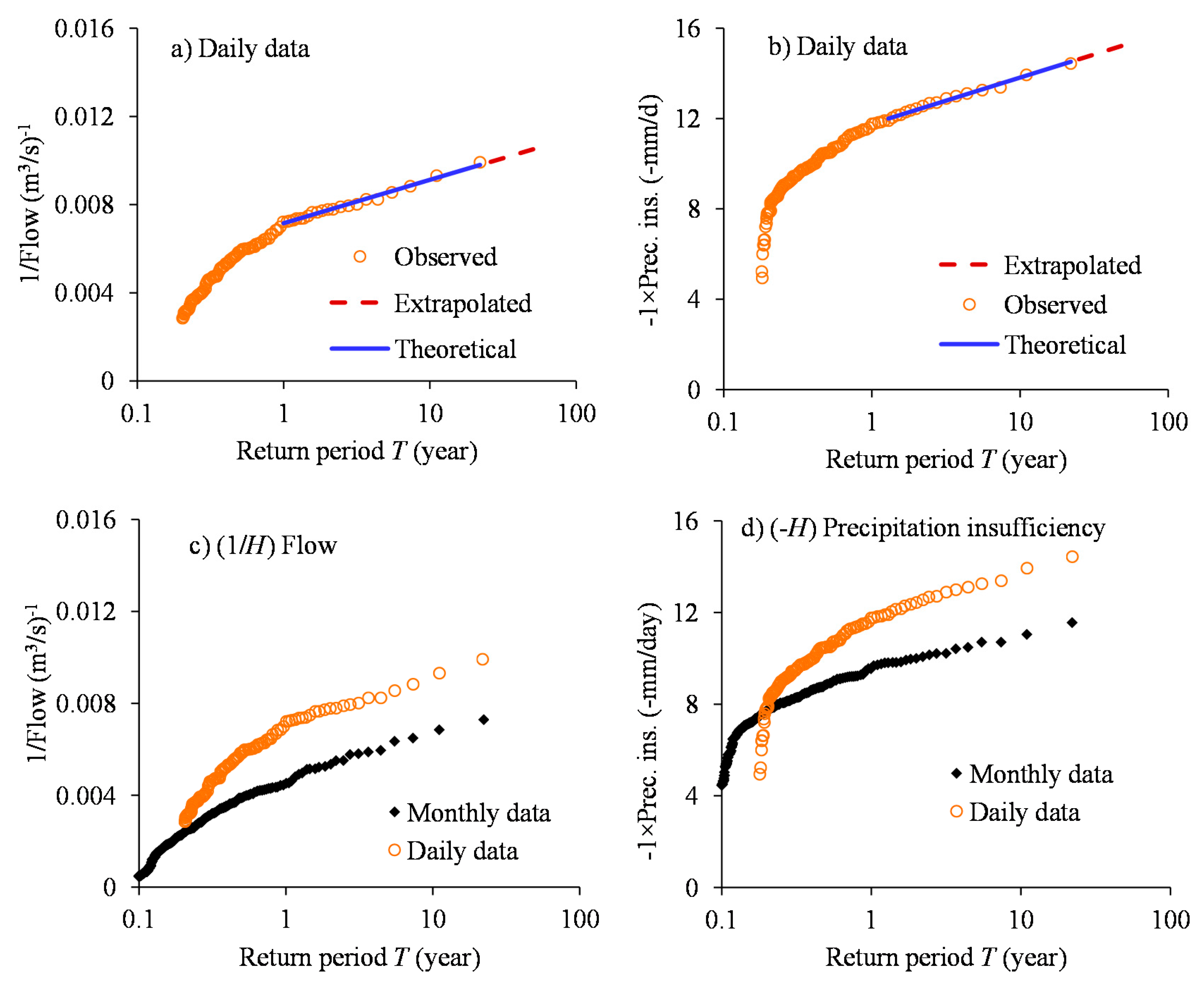
Figure 5.
Selected drought event based on the catchment-wide: (a) daily; and (b) monthly (H) precipitation insufficiency (Prec. ins.) from 1979–2000.
Figure 5.
Selected drought event based on the catchment-wide: (a) daily; and (b) monthly (H) precipitation insufficiency (Prec. ins.) from 1979–2000.
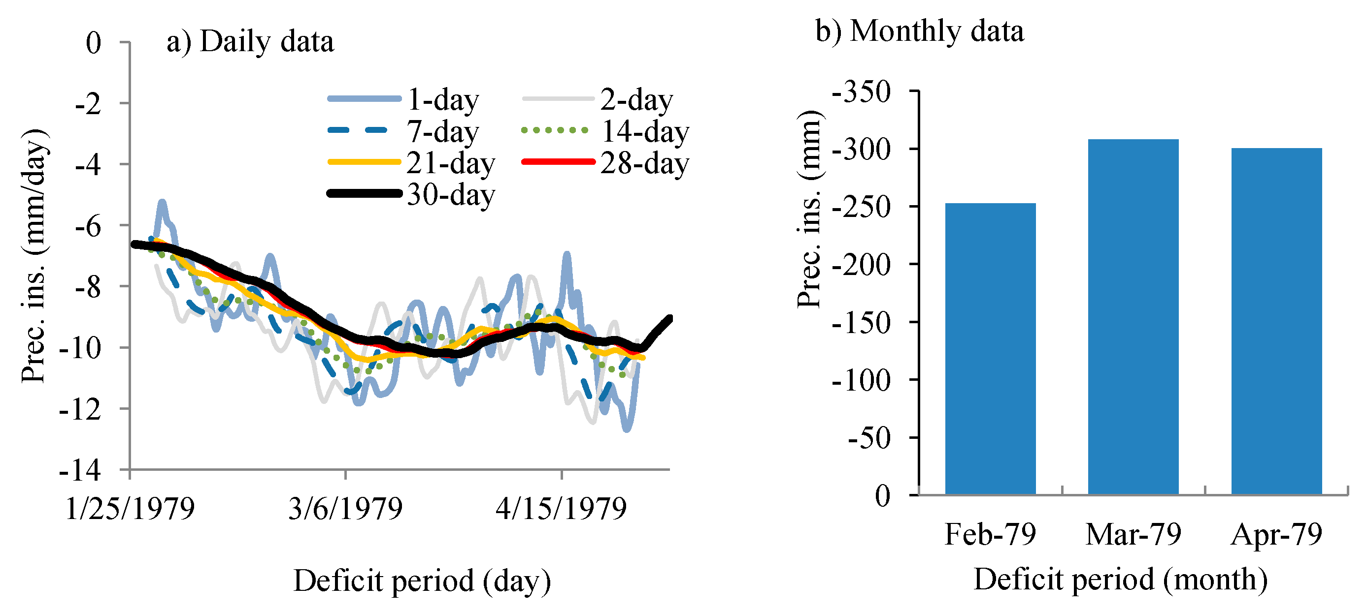
Figure 6.
POT events of (1/H) low flow from 1965 to 2002 at Khartoum based on: (a) daily; and (b) monthly data; as well as the POTs from basin-wide (−H) precipitation insufficiency for the period 1979–2000 based on: (c) daily; and (d) monthly data. The dotted line is a linear trend.
Figure 6.
POT events of (1/H) low flow from 1965 to 2002 at Khartoum based on: (a) daily; and (b) monthly data; as well as the POTs from basin-wide (−H) precipitation insufficiency for the period 1979–2000 based on: (c) daily; and (d) monthly data. The dotted line is a linear trend.

Figure 7.
POT events of (1/H) low flows versus: (a) RTO; and (b) return period. In the legend of (b), “CI” stands for confidence interval on the T-year events from “Method 2”. For chart (b), the horizontal axis is based on logarithmic scale.
Figure 7.
POT events of (1/H) low flows versus: (a) RTO; and (b) return period. In the legend of (b), “CI” stands for confidence interval on the T-year events from “Method 2”. For chart (b), the horizontal axis is based on logarithmic scale.
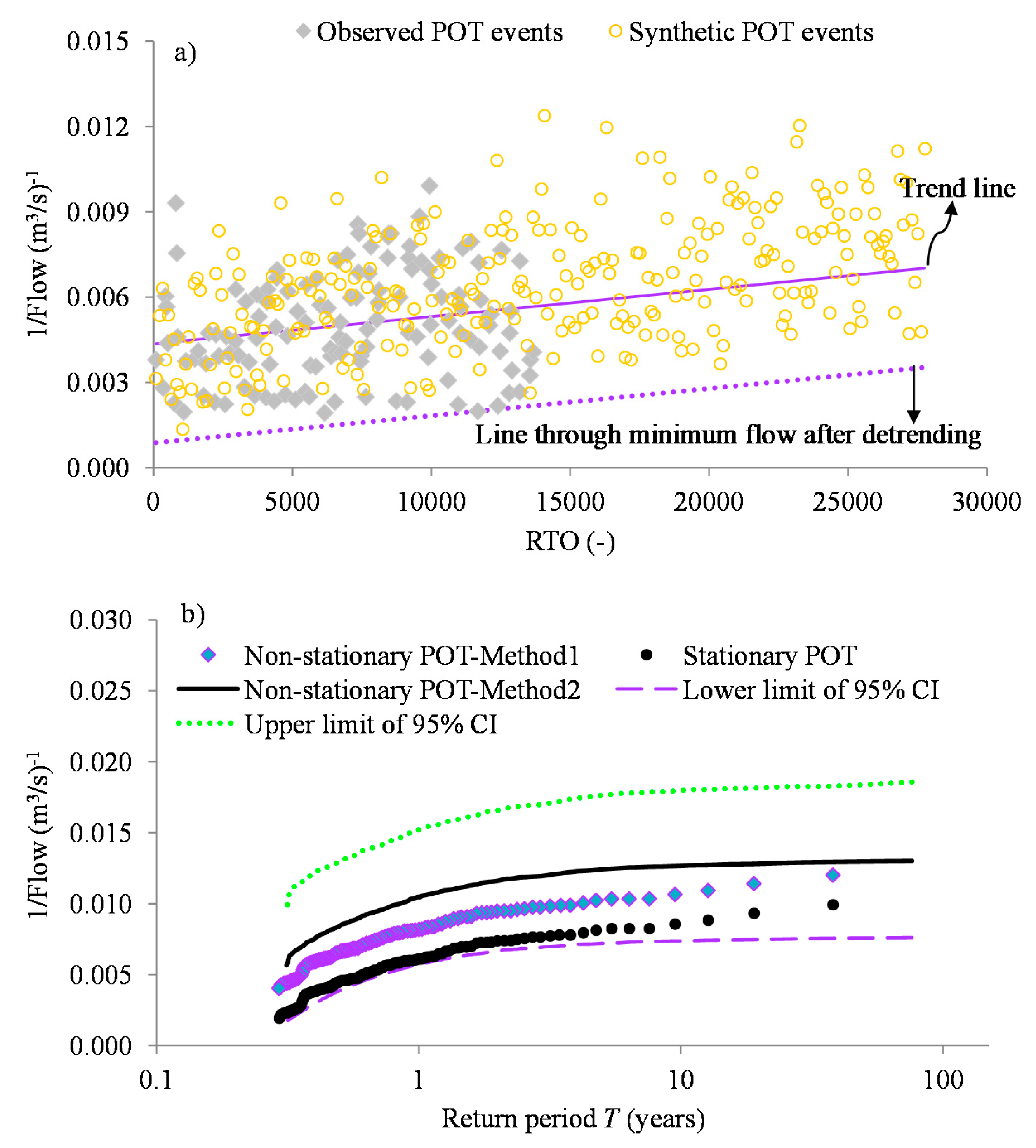
Figure 8.
Return period T against: (a) T-year low flow (H) after back-transformation from (1/H); and (b) bias on the T-year low flow (H).
Figure 8.
Return period T against: (a) T-year low flow (H) after back-transformation from (1/H); and (b) bias on the T-year low flow (H).

Figure 9.
Meteorological dry and wet conditions in terms of NPI and SPEI applied to catchment-wide: (a) daily; and (b) monthly precipitation insufficiency. Chart (c) shows NPI derived from daily river flow (H) and precipitation insufficiency (H). In each chart, the label text in “( )” shows the aggregation level.


Figure 10.
Meteorological dry and wet conditions in terms of: (a,c) SPEI; and (b,d) NPI applied to catchment-wide daily precipitation insufficiency. The label text in “( )” of the legend shows the aggregation level.
Figure 10.
Meteorological dry and wet conditions in terms of: (a,c) SPEI; and (b,d) NPI applied to catchment-wide daily precipitation insufficiency. The label text in “( )” of the legend shows the aggregation level.

Figure 11.
Skewness of SPEI when applied to daily precipitation insufficiency based on the aggregation level of: (a) one day; and (b) 180 days. The label text in “( )” of the legend shows the aggregation level.
Figure 11.
Skewness of SPEI when applied to daily precipitation insufficiency based on the aggregation level of: (a) one day; and (b) 180 days. The label text in “( )” of the legend shows the aggregation level.

Figure 12.
Extreme dry and wet conditions in terms of NPI and SPEI based on catchment-wide: (a) daily; and (b) monthly precipitation insufficiency over the period 1979–2002; and (c,d) the skewness of the indices based on daily and monthly precipitation insufficiency, respectively.
Figure 12.
Extreme dry and wet conditions in terms of NPI and SPEI based on catchment-wide: (a) daily; and (b) monthly precipitation insufficiency over the period 1979–2002; and (c,d) the skewness of the indices based on daily and monthly precipitation insufficiency, respectively.

Figure A1.
Rejection rate for (a,b) FGN; (c,d) DFBM; (e,f) FDP; and (g–l) ARFIMA models. Trend results obtained: (a,c,e,g,i,k) without; and (b,d,f,h,j,l) with TCSD variance correction for persistence. All the charts share the same legend as in (b).
Figure A1.
Rejection rate for (a,b) FGN; (c,d) DFBM; (e,f) FDP; and (g–l) ARFIMA models. Trend results obtained: (a,c,e,g,i,k) without; and (b,d,f,h,j,l) with TCSD variance correction for persistence. All the charts share the same legend as in (b).
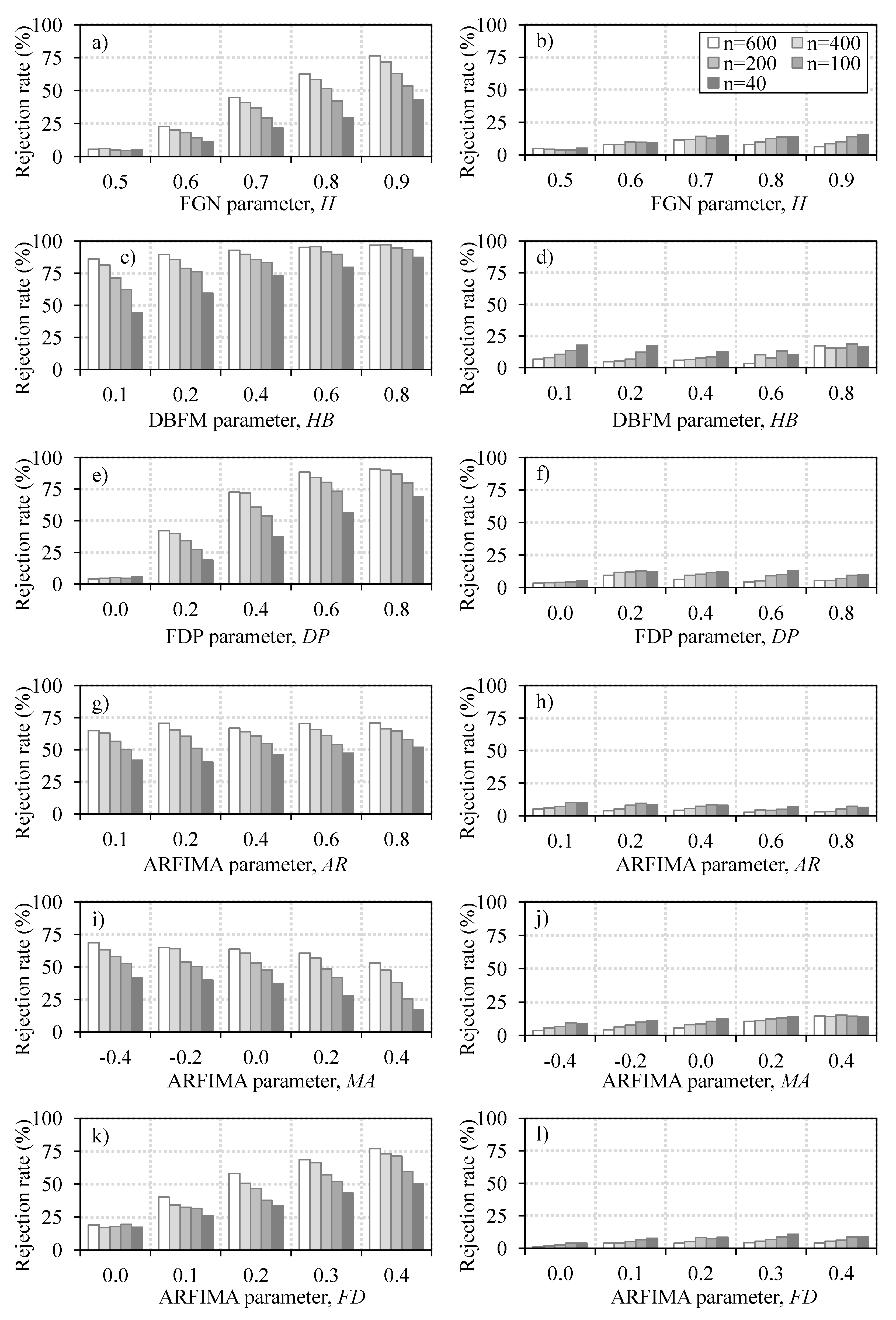
Figure A2.
Plots of: (a–i) synthetic series Xsyn of n = 200; and (1–9) the cumulative effects (Csum, Equation (A1)) of the temporal variations for the corresponding time series.
Figure A2.
Plots of: (a–i) synthetic series Xsyn of n = 200; and (1–9) the cumulative effects (Csum, Equation (A1)) of the temporal variations for the corresponding time series.

Figure A3.
Hydro-climatic deficit periods based on daily: (a) flow; and (b) precipitation insufficiency.
Figure A3.
Hydro-climatic deficit periods based on daily: (a) flow; and (b) precipitation insufficiency.
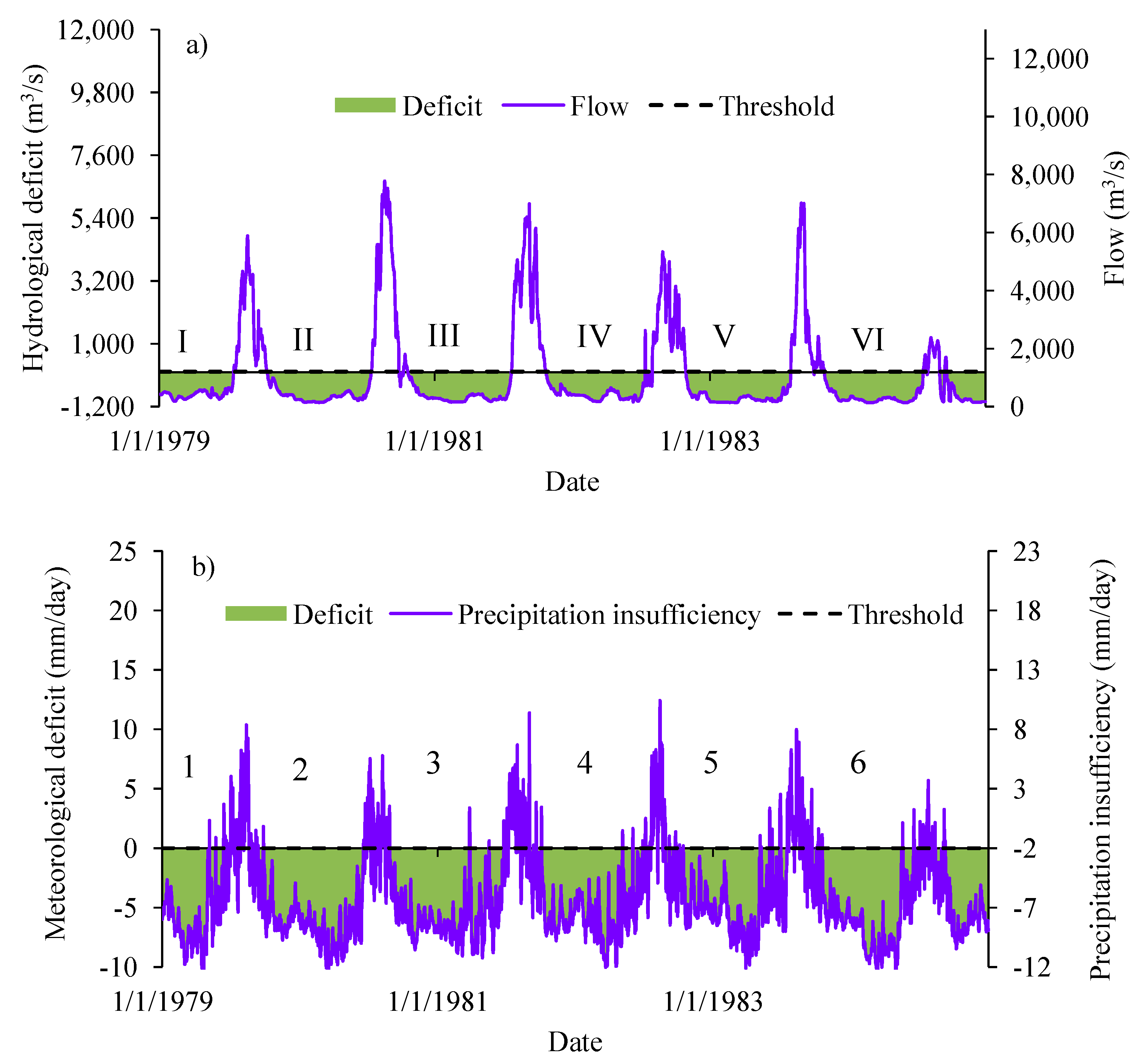
Figure A4.
Absolute Meteorological Deficit Sum (MDS) for a selected drought event.
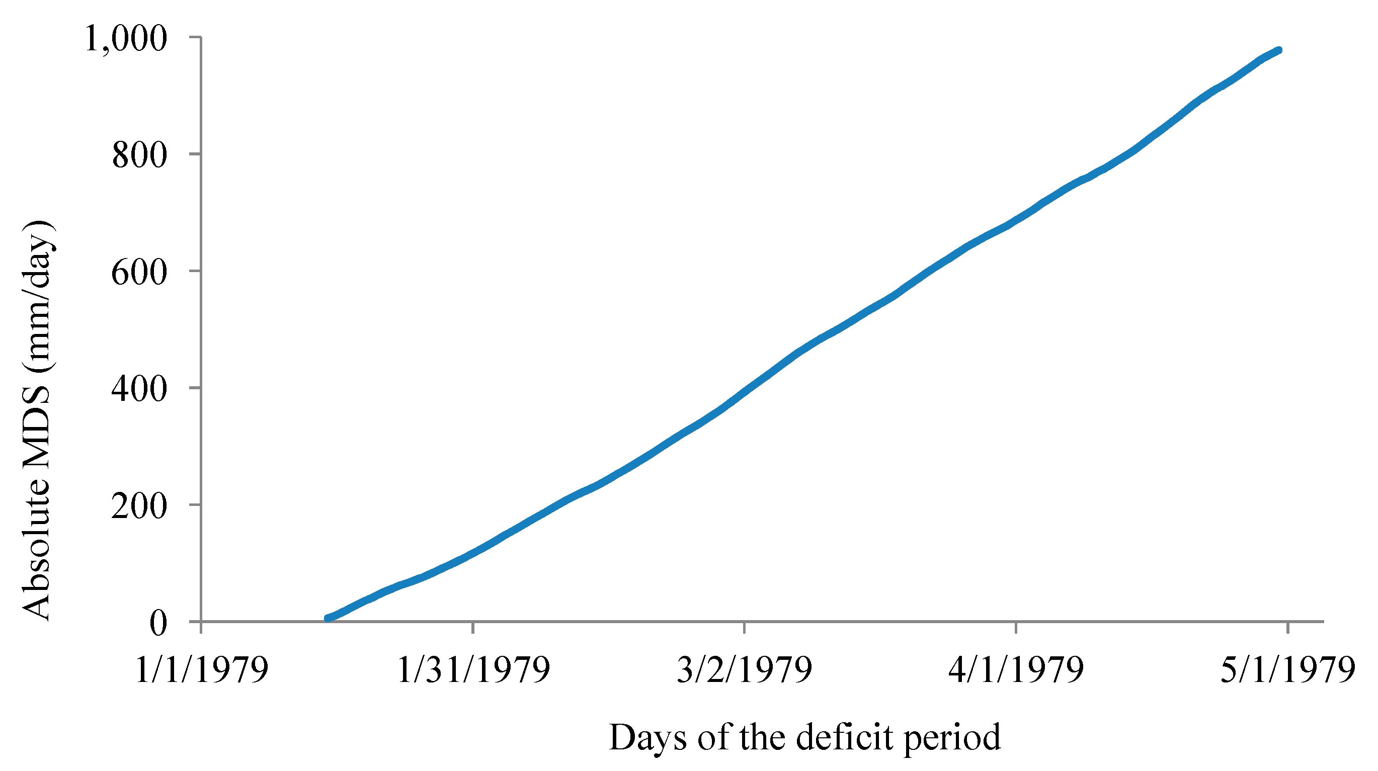
Figure A5.
Meteorological deficit of: (a,b) mild; (c) severe; and (d) extreme drought quantile category. In the legend, e.g., T5 stands for return period of 5 years.
Figure A5.
Meteorological deficit of: (a,b) mild; (c) severe; and (d) extreme drought quantile category. In the legend, e.g., T5 stands for return period of 5 years.
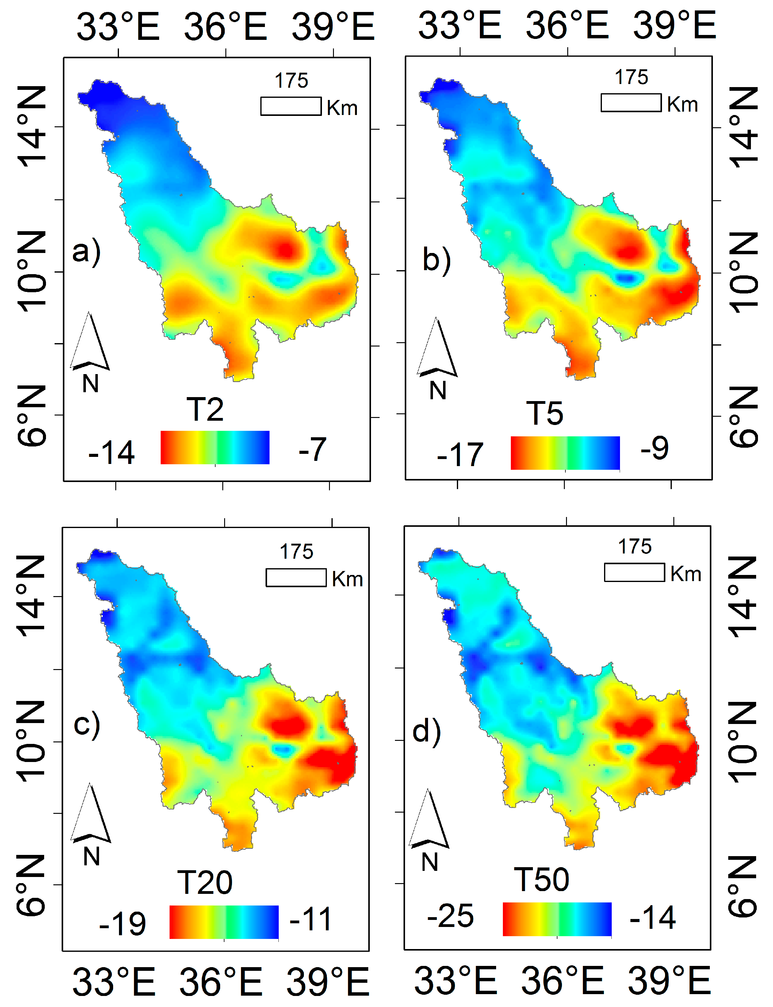
Figure A6.
Historical: (a,b) incidence (%); and (c,d) LDP (day) of the precipitation insufficiency based on threshold of: (a,c) −10 mm/day; and (b,d) −5 mm/day, considering the period 1979–2000.
Figure A6.
Historical: (a,b) incidence (%); and (c,d) LDP (day) of the precipitation insufficiency based on threshold of: (a,c) −10 mm/day; and (b,d) −5 mm/day, considering the period 1979–2000.

Figure A7.
IDT relationships for: (a) hydrological drought; and (c) meteorological drought. LDP-DT relationships for: (b) hydrological drought; and (d) meteorological drought.
Figure A7.
IDT relationships for: (a) hydrological drought; and (c) meteorological drought. LDP-DT relationships for: (b) hydrological drought; and (d) meteorological drought.

Figure A8.
T-year events comprising: (a) LFDF relationships; and (b) MIDF relationship. For chart (a), the T-year events considering stationarity and non-stationarity are presented in the form of lines and markers, respectively. In the legend, e.g., T5 denotes T-year curve for T = 5 years.
Figure A8.
T-year events comprising: (a) LFDF relationships; and (b) MIDF relationship. For chart (a), the T-year events considering stationarity and non-stationarity are presented in the form of lines and markers, respectively. In the legend, e.g., T5 denotes T-year curve for T = 5 years.
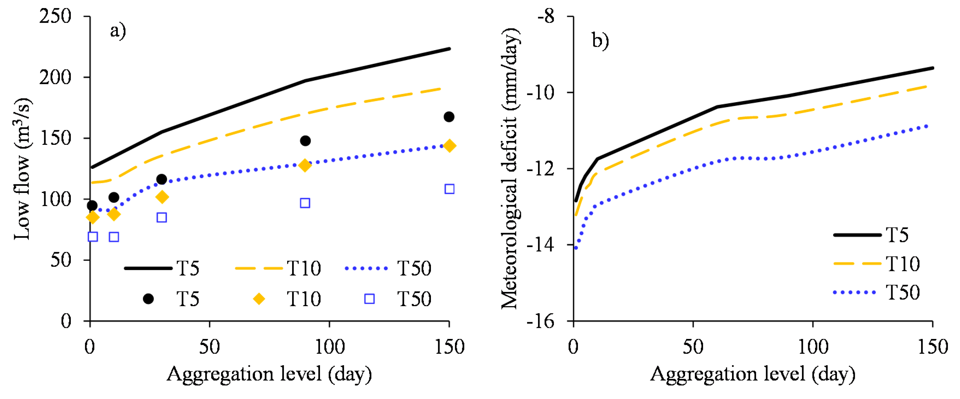
Figure A9.
Hydrological dry spell–duration–frequency relationships.

Figure A10.
(a) Hydrological drought; (b) sum of meteorological deficit; and (c) comparison of the sum of hydrological and meteorological deficits.
Figure A10.
(a) Hydrological drought; (b) sum of meteorological deficit; and (c) comparison of the sum of hydrological and meteorological deficits.

Figure A11.
Hydrological deficit versus: (a) sum of precipitation insufficiency; and (b) deficit period.
Figure A11.
Hydrological deficit versus: (a) sum of precipitation insufficiency; and (b) deficit period.

Figure A12.
Hydrological response constant (HRC) versus: (a) hydrological deficit; and (b) duration.
Figure A12.
Hydrological response constant (HRC) versus: (a) hydrological deficit; and (b) duration.


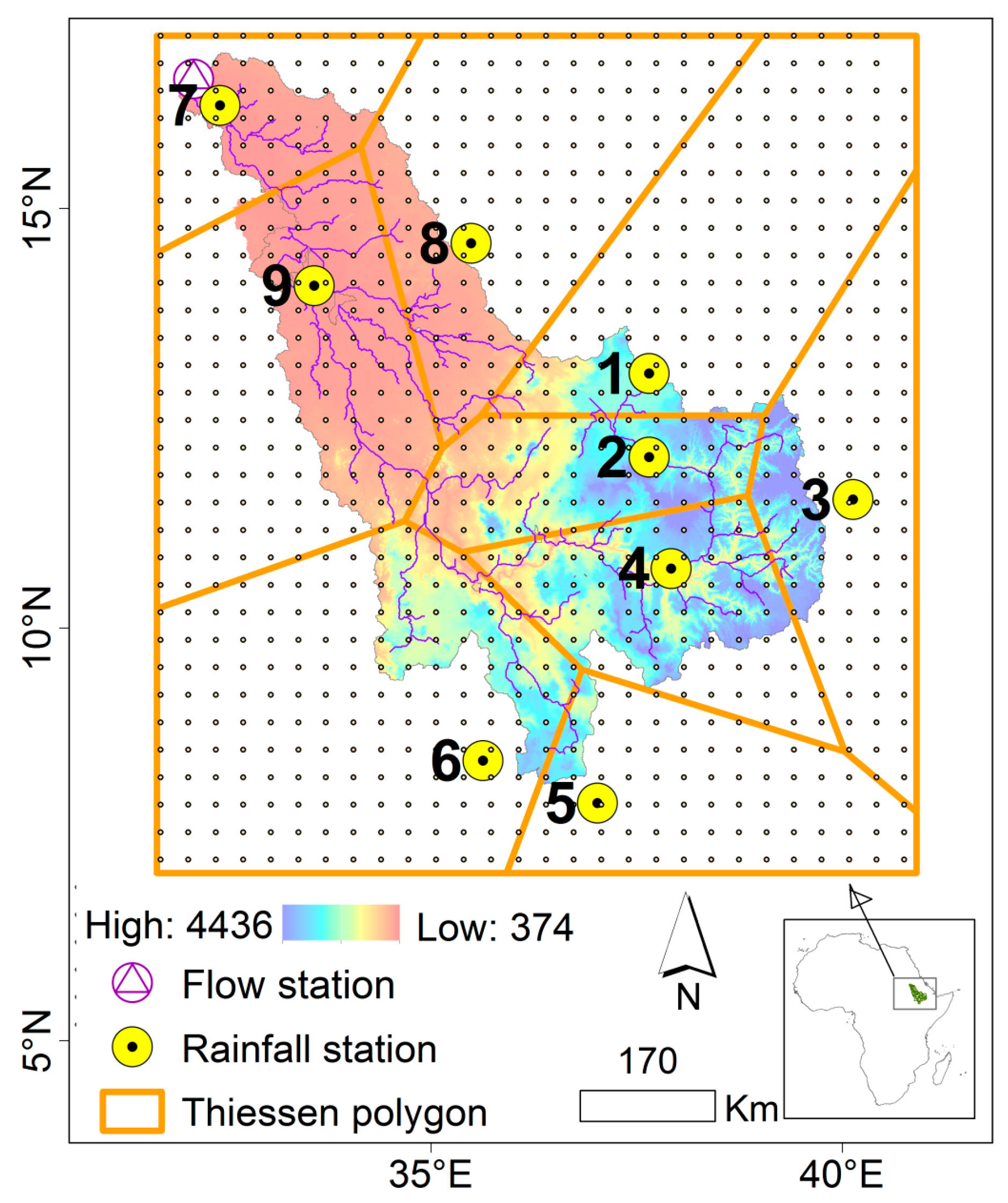
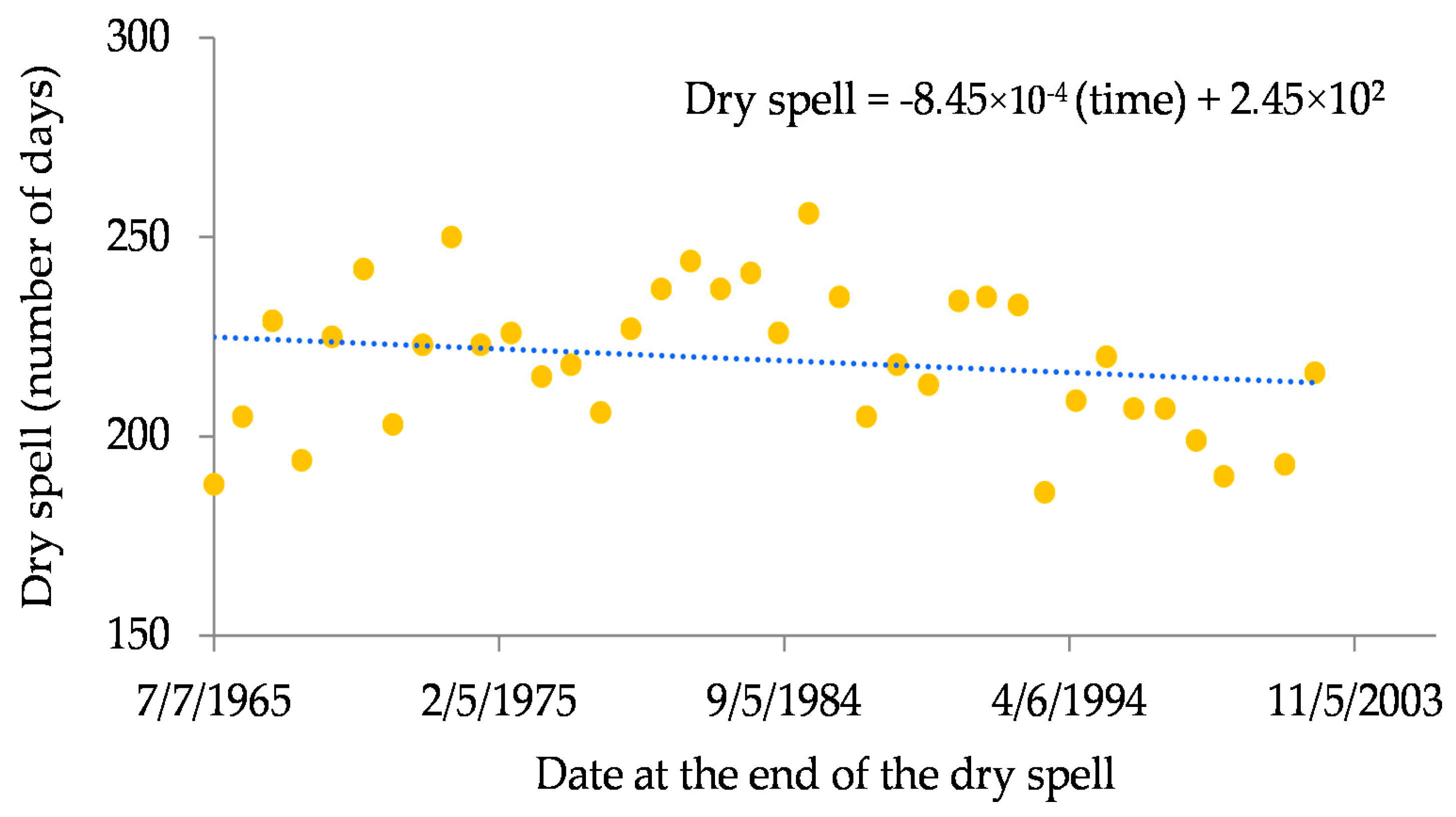
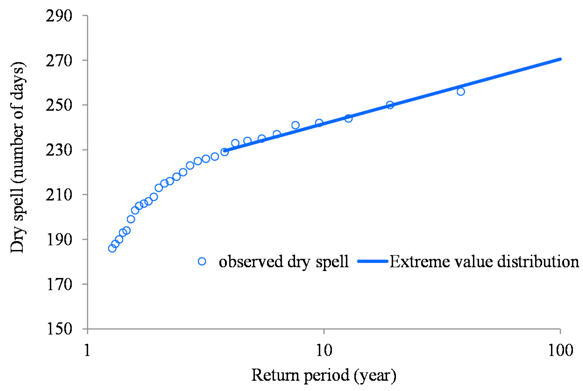
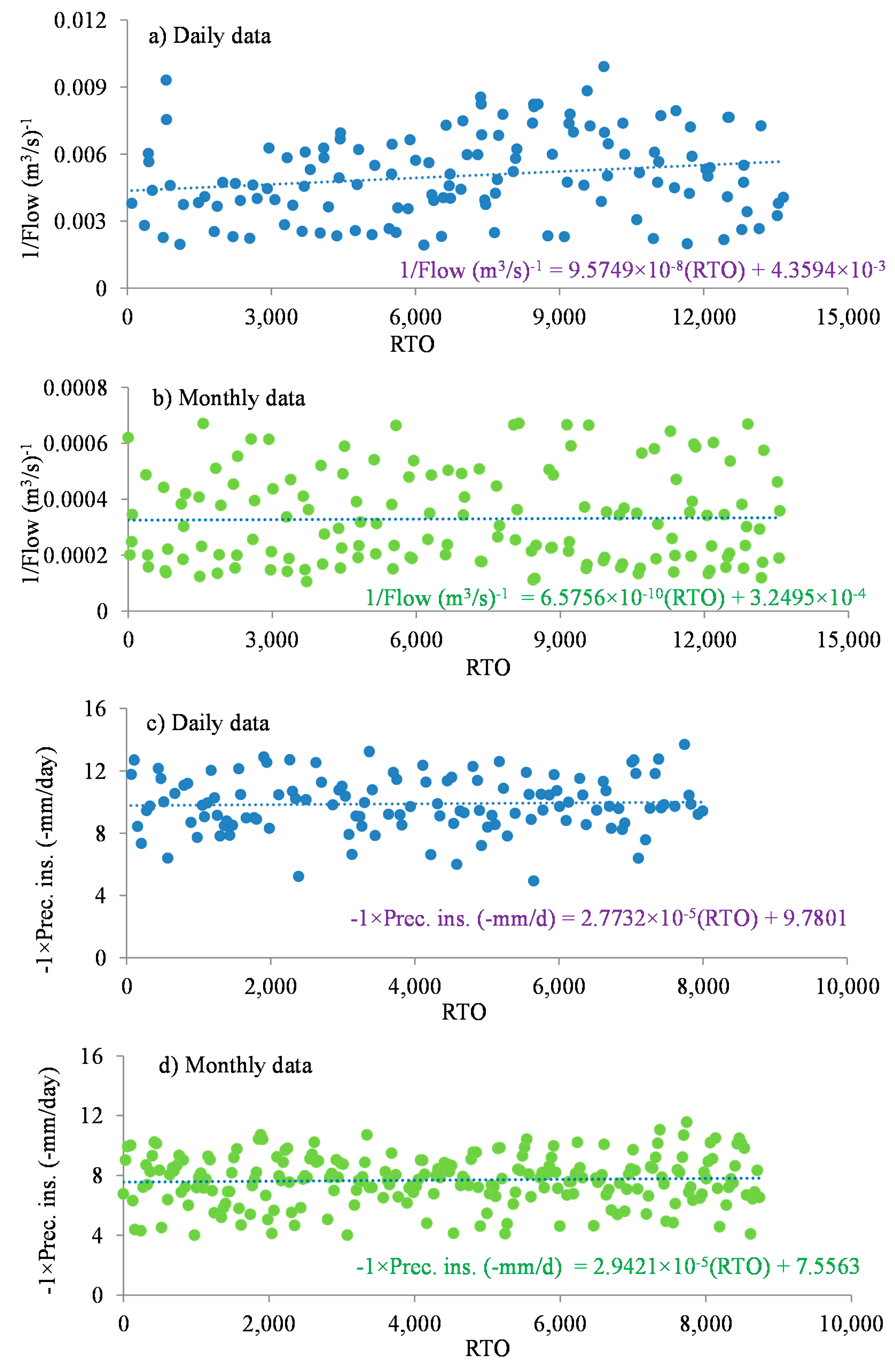
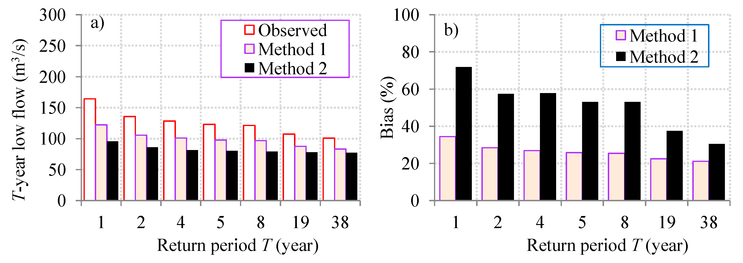
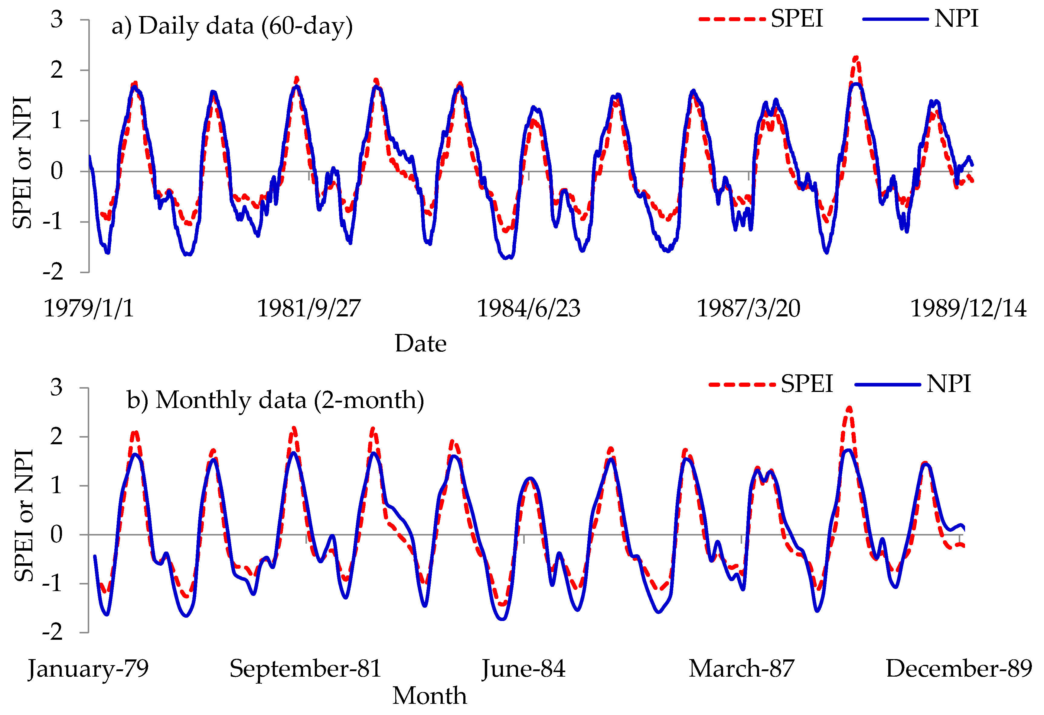
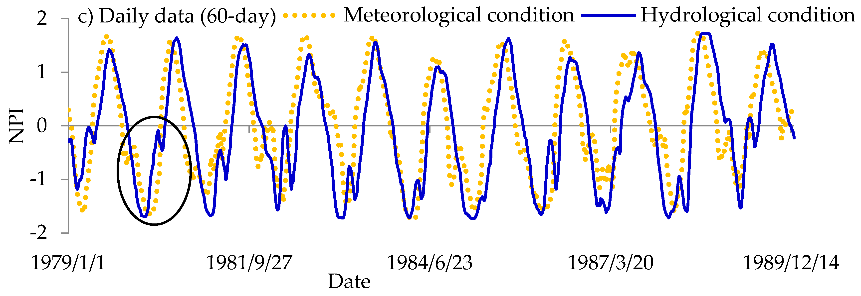
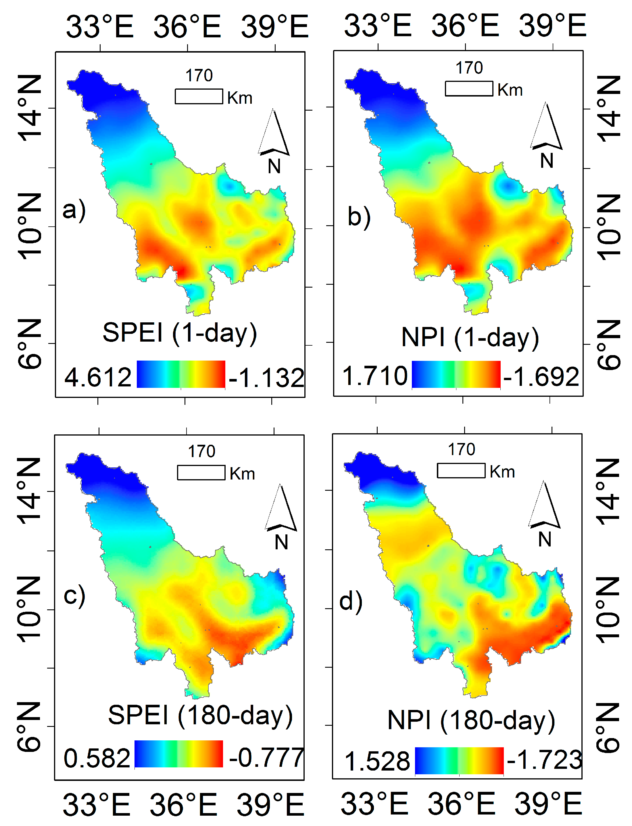
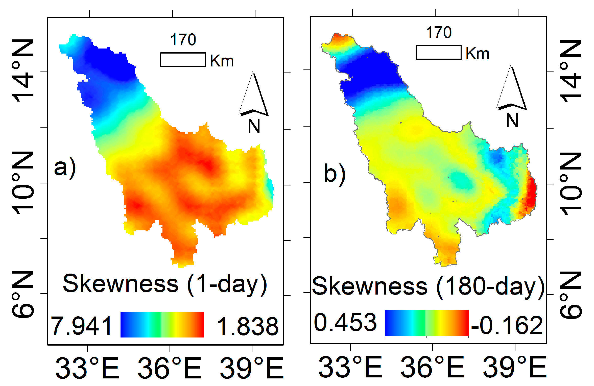
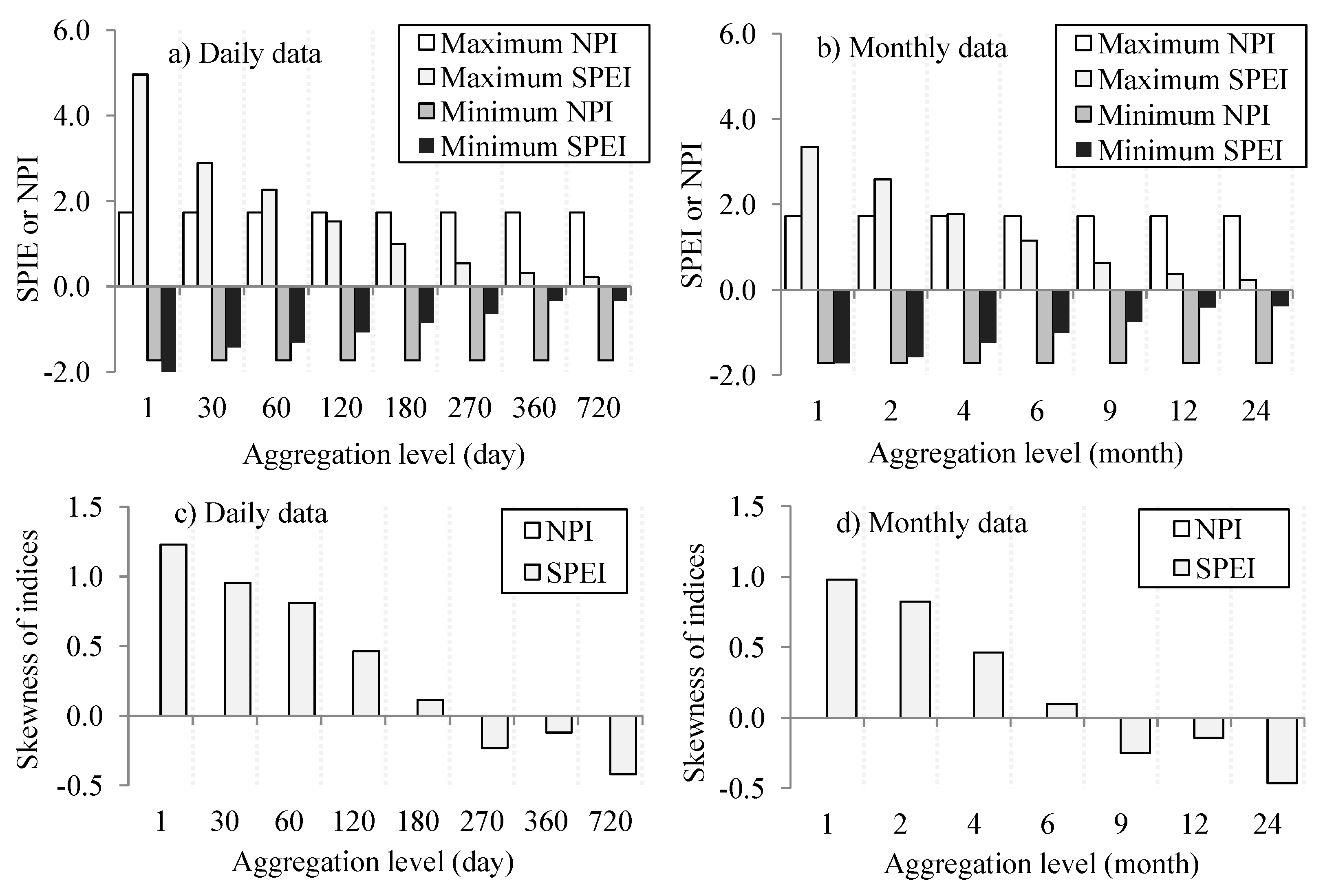
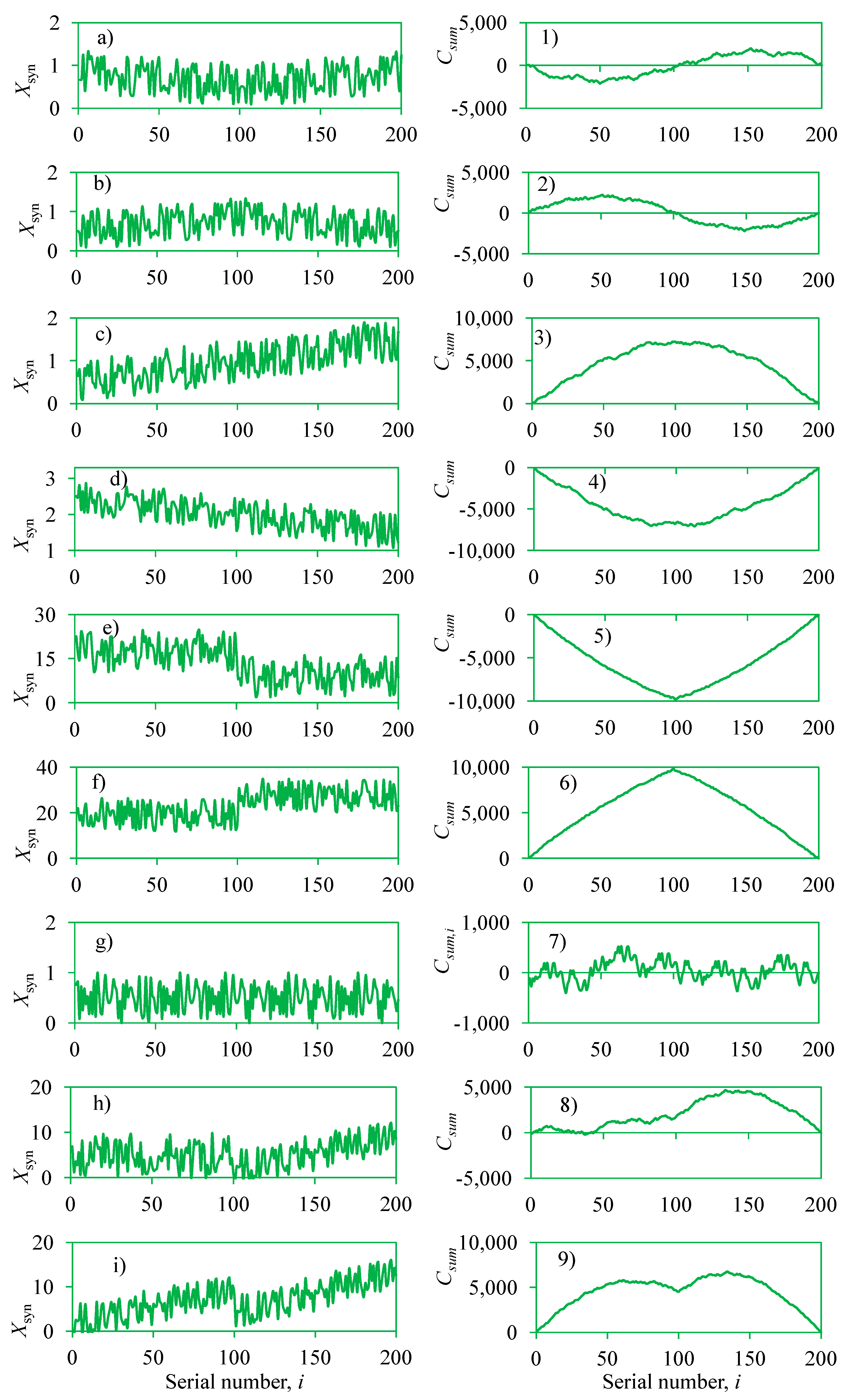
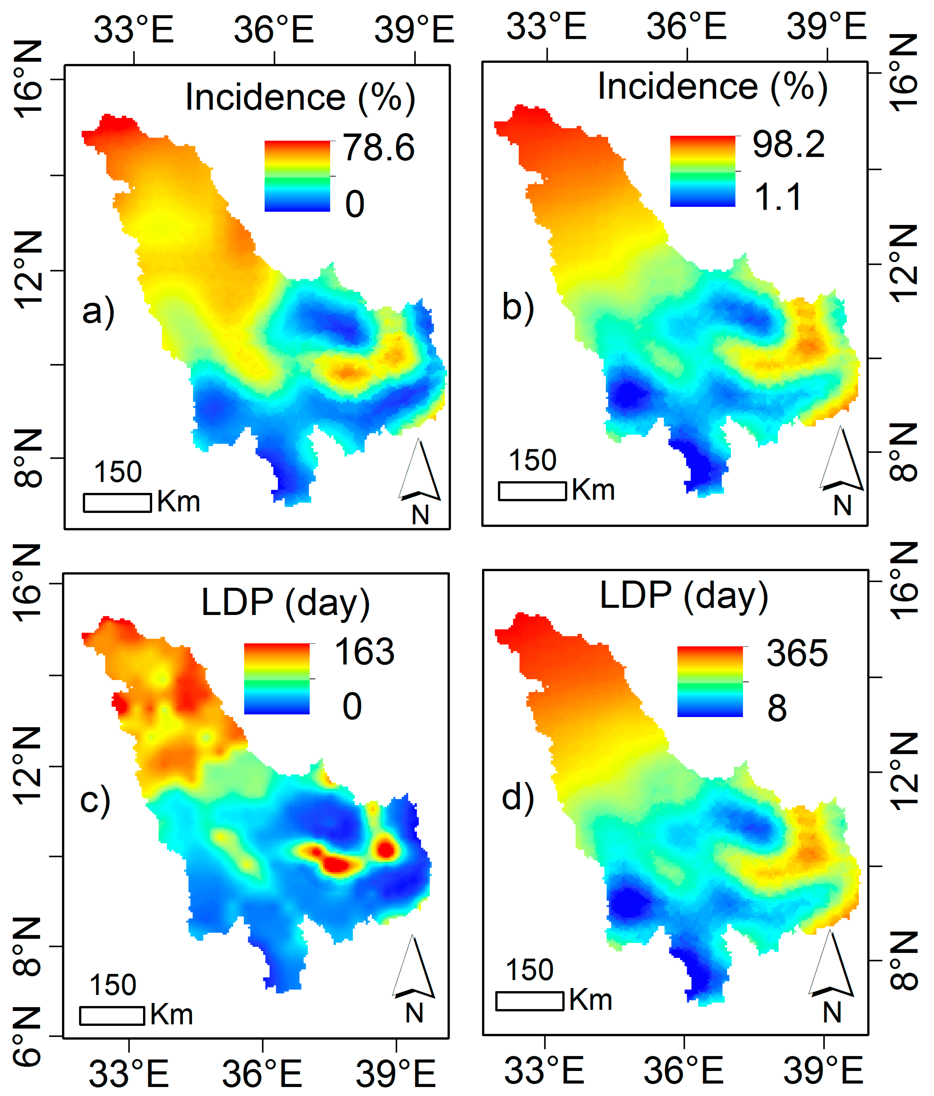
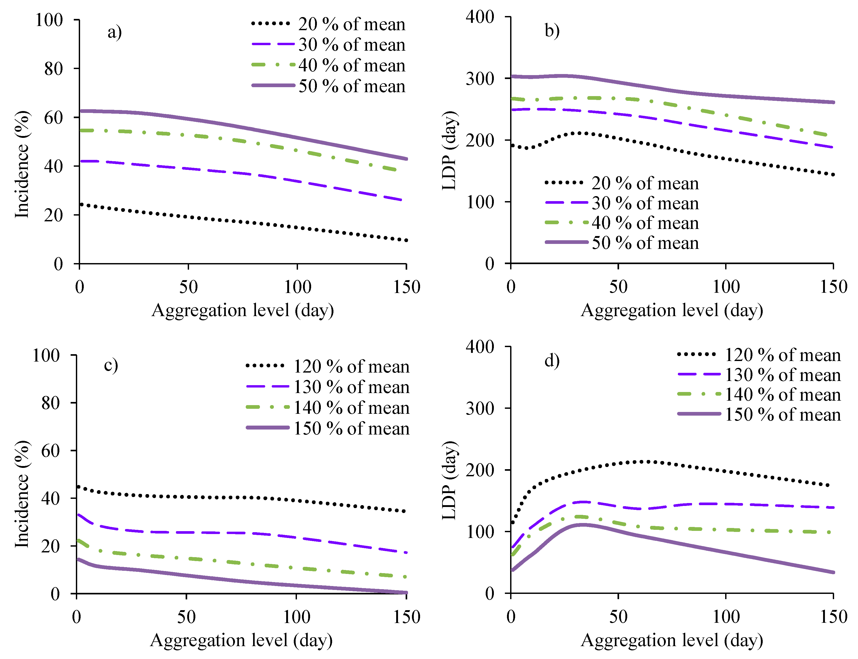
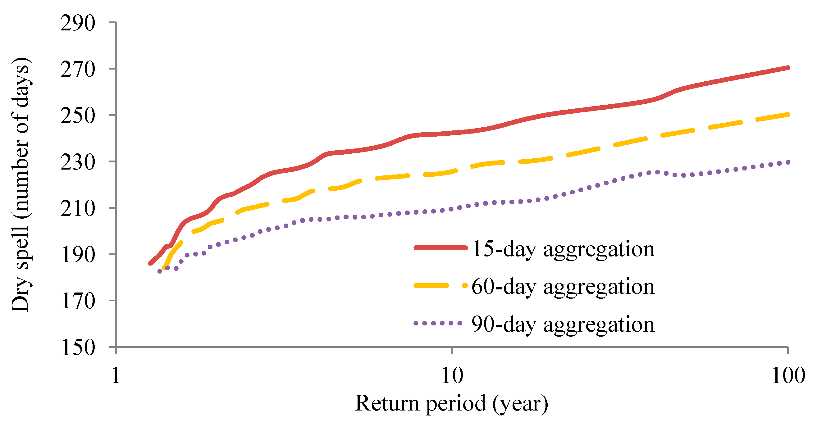
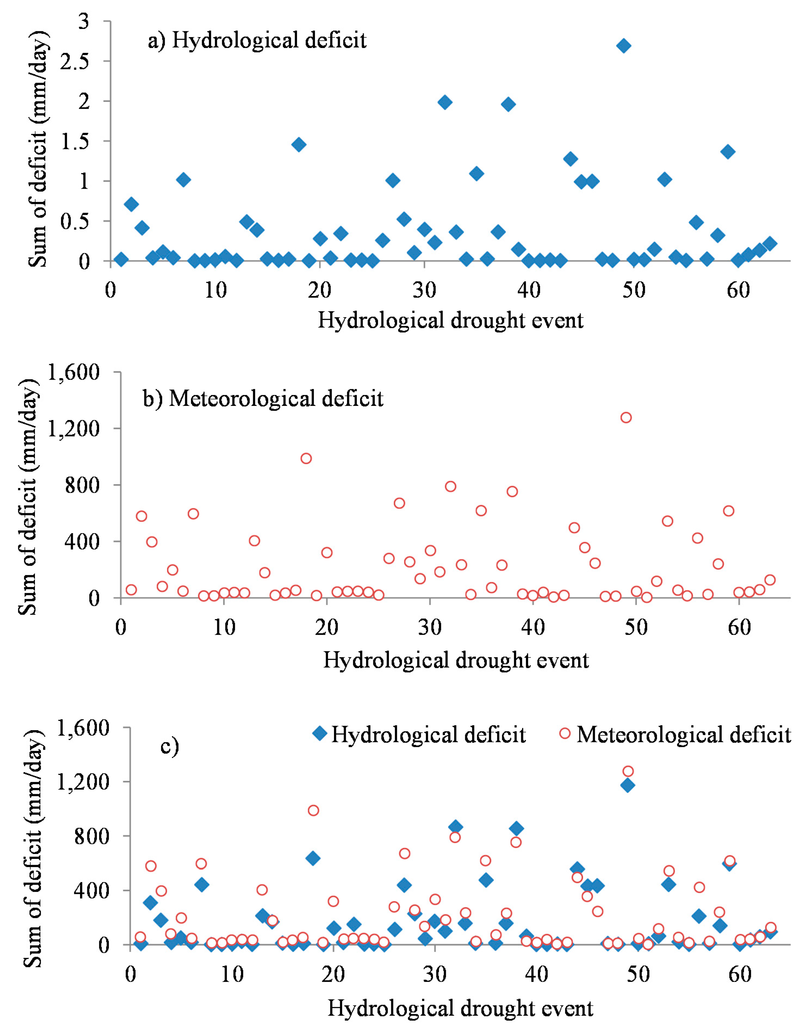
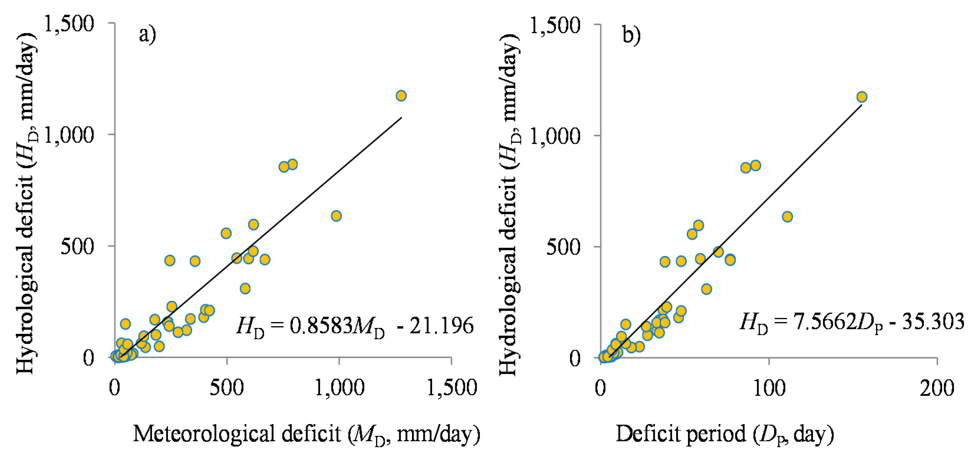
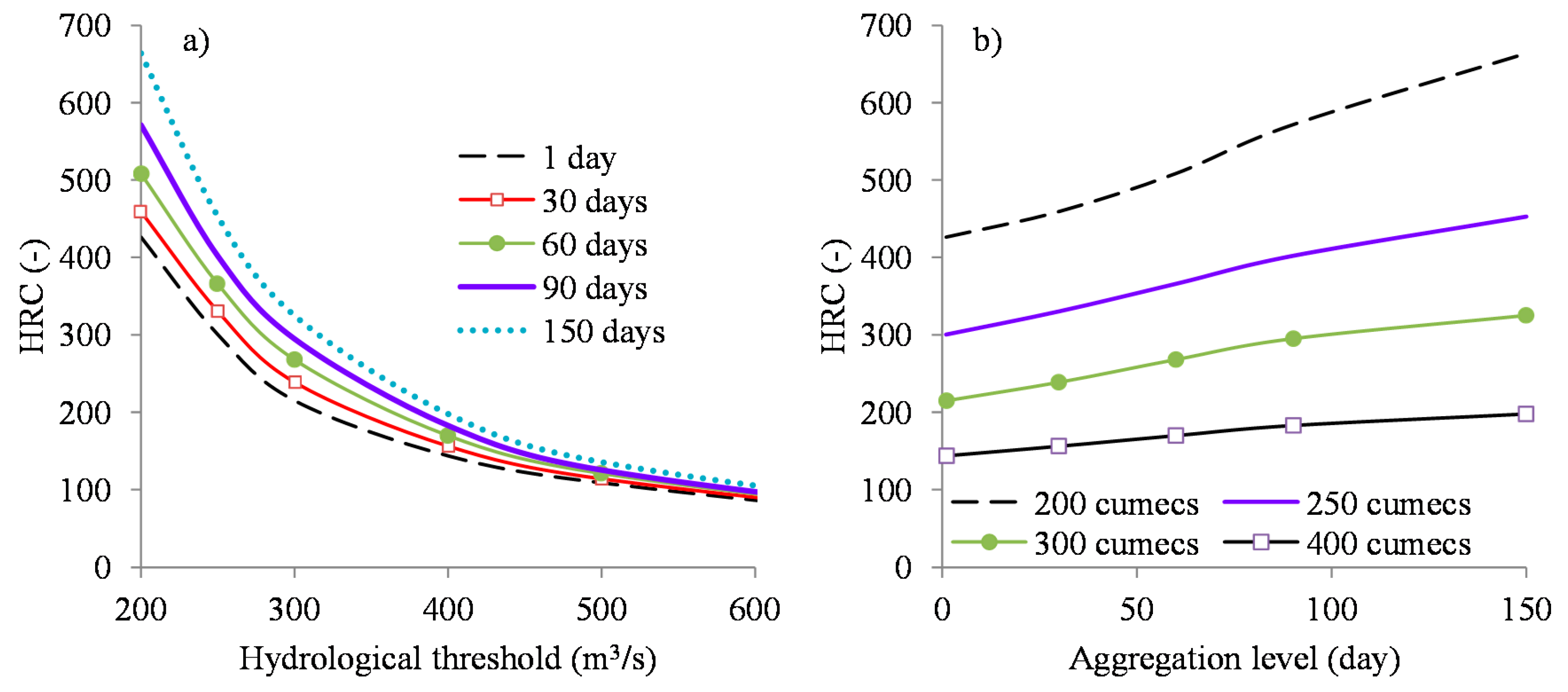
Table 1.
Overview of meteorological stations and rainfall data.
| Station | Period | Statistics | ||||
|---|---|---|---|---|---|---|
| Number | Identity | Name | From | To | CV | Skewness |
| 1 | ET000063331 | Gondar | 1952 | 1988 | 2.30 | 3.63 |
| 2 | ET000063332 | Bahar Dar | 1952 | 1988 | 2.53 | 4.57 |
| 3 | ET000063333 | Combolcha | 1953 | 1988 | 2.54 | 3.98 |
| 4 | ET000063334 | Debremarcos | 1953 | 1987 | 1.94 | 2.93 |
| 5 | ET000063402 | Jimma | 1952 | 1988 | 1.92 | 3.11 |
| 6 | ET000063403 | Gore | 1952 | 2014 | 1.95 | 3.40 |
| 7 | SU000062721 | Khartoum | 1957 | 1987 | 8.31 | 13.66 |
| 8 | SU000062752 | Gedaref | 1957 | 1976 | 4.37 | 8.21 |
| 9 | SU000062762 | Sennar | 1961 | 2013 | 6.17 | 11.22 |
Table 2.
Decision on whether to consider non-stationarity for frequency analysis.
| Decision | Trend Magnitude | ||
|---|---|---|---|
| m ≠ 0 | m ≈ 0 | ||
| Trend direction | |Z*| ≥ |Zαs/2| | Non-stationarity | Stat * |
| |Z*| < |Zαs/2| | Non-stationarity | Stationarity | |
Stat *: If the trend slope is not significantly different from zero at a selected αs%, but for practical reason there is need to take the trend magnitude into decision making perspective, non-stationarity should be considered; otherwise, frequency analysis should be conducted assuming analogy to realizations from a stationary process. Furthermore, m ≠ 0: means that for (1/H) flow or (−H) precipitation insufficiency, m > 0. Thus, after back-transformation of the data, i.e., for (H) flow or (H) precipitation insufficiency, the trend slope becomes m < 0. However, in flood frequency analyses for which data transformation is not required, the concern is on m > 0 for the significance of both trend direction and magnitude detected using (H) flow or (H) precipitation insufficiency. Finally, Z*: means ZCSD or ZMK or the standardized trend statistic of the method used.
Table 3.
Categorization of drought indices.
| Daily Time Scale | Monthly Time Scale | Category | Return Period T (year) | ||
|---|---|---|---|---|---|
| From | To | From | To | ||
| 0 | −1.72258 | 0 | −1.44421 | Near normal | ≤1 |
| −1.72259 | −1.73112 | −1.44422 | −1.70391 | Mild | 2–9 |
| −1.73113 | −1.73159 | −1.70392 | −1.71833 | Moderate | 10–19 |
| −1.73160 | −1.73188 | −1.71834 | −1.72169 | Severe | 20–49 |
| −1.73189 | −1.73197 | −1.72170 | −1.72988 | Extreme | 50–99 |
| −1.73198 | <−1.73198 | −1.72989 | <−1.72989 | Exceptional | ≥100 |
When the negative indices are replaced by the absolute values, and the “<” changed to “>” for the indices of the exceptional case of wetness, the same categorization applies for wet conditions.
Table 4.
Statistical results on the analysis of trend magnitude (m).
| POT | Data Period | Daily Data | Monthly Data | ||
|---|---|---|---|---|---|
| m | p-Value | m | p-Value | ||
| (1/H) low flow | 1965–2002 | 9.57 × 10⁻⁸ | 0.007 | 6.58 × 10⁻¹⁰ | 0.843 |
| (1/H) low flow | 1979–2000 | 1.64 × 10⁻⁷ | 0.152 | −3.85 × 10⁻⁹ | 0.622 |
| (-H) precipitation insufficiency | 1979–2000 | 2.77 × 10⁻⁵ | 0.685 | 2.94 × 10⁻⁵ | 0.480 |
Table 5.
Statistical results on the analysis of trend direction.
| POT | Data Period | p-Value From | p-Value From | ||
|---|---|---|---|---|---|
| Daily Data | Monthly Data | ||||
| CSD Test | MK Test | CSD Test | MK Test | ||
| (1/H) low flow | 1965–2002 | 0.151 | 0.136 | 0.998 | 0.985 |
| (1/H) low flow | 1979–2000 | 0.375 | 0.413 | 0.914 | 0.937 |
| (-H) precipitation insufficiency | 1979–2000 | 0.497 | 0.511 | 0.977 | 0.963 |
© 2017 by the author. Licensee MDPI, Basel, Switzerland. This article is an open access article distributed under the terms and conditions of the Creative Commons Attribution (CC BY) license (http://creativecommons.org/licenses/by/4.0/).
Share and Cite
MDPI and ACS Style
Onyutha, C. On Rigorous Drought Assessment Using Daily Time Scale: Non-Stationary Frequency Analyses, Revisited Concepts, and a New Method to Yield Non-Parametric Indices. Hydrology 2017, 4, 48. https://doi.org/10.3390/hydrology4040048
AMA Style
Onyutha C. On Rigorous Drought Assessment Using Daily Time Scale: Non-Stationary Frequency Analyses, Revisited Concepts, and a New Method to Yield Non-Parametric Indices. Hydrology. 2017; 4(4):48. https://doi.org/10.3390/hydrology4040048
Chicago/Turabian StyleOnyutha, Charles. 2017. "On Rigorous Drought Assessment Using Daily Time Scale: Non-Stationary Frequency Analyses, Revisited Concepts, and a New Method to Yield Non-Parametric Indices" Hydrology 4, no. 4: 48. https://doi.org/10.3390/hydrology4040048
Note that from the first issue of 2016, this journal uses article numbers instead of page numbers. See further details here.