AI-Integrated Framework for Designing Optimized Groundwater Level Observation Networks Based on Hybrid Machine Learning and Stochastic Simulation Frameworks

Abstract

This study develops an integrated framework combining groundwater numerical modeling, probabilistic simulation, and machine learning to optimize the spatial design of an Optimized Groundwater Level Observation Network (OGLON) in the Mareth basin. A total of 565 existing monitoring wells were used to calibrate the groundwater flow model, complemented by stochastic groundwater simulations to train two AI-based approaches: the AI-Assisted Centroid Clustering (AIACC) algorithm and the Data-Driven Sparse Bayesian Learning (DDSBL) model. Three OGLON configurations were generated, AIACC (30 wells), DDSBL (30 wells), and Refined-DDSBL (30 wells), and benchmarked against the current monitoring network. Model performance indicates that the AIACC configuration reduces model error from 17,232 to 31.30, achieving an RMSE of 0.2145 m, significantly outperforming both the existing network (RMSE 0.5028 m) and the original DDSBL system (RMSE 0.6678 m). The Refined-DDSBL configuration provides the best overall accuracy, reducing model error from 21,355 to 1.32 and achieving the lowest RMSE (0.0153 m) and MAE (0.0091 m). Groundwater levels simulated under the proposed networks range between 3.8 m and 94.7 m, with the AIACC and Refined-DDSBL approaches offering improved spatial representation of key hydrogeological patterns compared to existing wells. Overall, results demonstrate a clear trade-off between computational efficiency (AIACC) and maximum predictive accuracy (Refined-DDSBL). Both AIACC and Refined-DDSBL significantly enhance spatial coverage and groundwater representation, confirming the effectiveness of integrating machine learning with groundwater modeling for cost-efficient and high-performance OGLON design.

1. Introduction

Groundwater serves as a vital resource, supplying water to diverse ecological and industrial systems while simultaneously facilitating the movement of pollutants through subsurface environments [1,2,3,4,5]. Deterioration in both the amount and purity of groundwater poses serious risks to public health and ecosystems, underscoring the critical need for continuous monitoring to ensure its sustainable management and protection [6,7,8]. The effectiveness of groundwater observation systems, composed of clustered or distributed sampling sites, depends on both the choice of locations and the timing of measurements [7,8,9]. Despite high costs and practical challenges [10,11], well networks provide essential data for building reliable groundwater models that improve aquifer understanding and forecasting [6,7,10]. Data from well-designed monitoring frameworks reveal spatial-temporal variations and improve model accuracy for simulating groundwater responses to environmental and human impacts [12,13,14].

Optimized groundwater level observation systems are essential for accurate aquifer modeling and effective resource management [15,16,17]. However, their design and assessment remain limited, often hindered by financial constraints and the lack of analytical tools to identify suitable well locations [7,9,14,16,17]. Groundwater observation design has evolved from traditional hydrogeological approaches, emphasizing aquifer properties and groundwater–surface water interactions, to data-driven, analytical frameworks [18,19,20]. Modern methods incorporate statistical, computational, and multi-criteria optimization techniques to improve spatial coverage and performance of monitoring systems [8,9,11,13,15,17].

Groundwater level monitoring network design has evolved from standard hydrogeological and geostatistical approaches that aim to capture aquifer dynamics while managing costs [8,15,21,22]. Conventional methods, such as uniform or systematic sampling, kriging, and multi-criteria analysis, use prior knowledge of aquifer properties, flow, and spatial variability to optimize site allocation [23,24,25,26]. Although structured and hydrogeologically grounded, these approaches often face notable limitations [8,9,15,17,23,24]. These methods may create redundant wells, overlook complex spatial–temporal patterns, and poorly adapt to changing groundwater conditions. Optimizing network density with minimal uncertainty also requires costly and time-consuming fieldwork and simulations [8,15,21,22].

Recent computational advances have made AI and ML powerful tools for monitoring network design [8,9,11,13,15,17]. Unlike conventional methods, these models can handle large datasets, learn complex patterns, and optimize networks with minimal human input. ML helps identify high-value wells, reduce redundancy, and improve predictive accuracy [15,17,27], while incorporating uncertainties, adapting to evolving aquifers, and balancing objectives like cost, accuracy, and coverage [15]. Standard approaches, such as kriging, multi-criteria decision analysis, and numerical simulations, remain useful for structured, physically interpretable insights but are limited by assumptions of linearity and static conditions [8,15,21,22].

AI/ML models commonly used for groundwater network design include Support Vector Machines (SVMs), Random Forests (RF), and Artificial Neural Networks (ANNs) [8,9,11,13,15,27]. SVMs optimize well placement by maximizing information gain [27,28]; RFs manage non-linear interactions and rank sites by predictive contribution [15,29]; and ANNs model complex multi-dimensional relationships for adaptive network optimization [7,8,30]. These approaches, however, require large, high-quality datasets, are computationally demanding, and are less interpretable than conventional hydrogeological methods [7,8,15].

Optimization of groundwater monitoring networks increasingly relies on hybrid and AI-enhanced approaches, which combine computational and statistical methods to improve efficiency and accuracy [31,32,33,34]. These models integrate conventional hydrogeological knowledge with AI/ML capabilities, enabling multiple objectives, minimizing costs, reducing redundancy, capturing spatial heterogeneity, and lowering predictive uncertainty, while dynamically adapting to changing aquifer conditions [31,32,33,34].

AI-assisted frameworks, such as the AI-Assisted Centroid Clustering (AIACC) algorithm, highlight the benefits of hybrid approaches. AIACC optimizes well placement by grouping areas with similar hydrogeological properties and selecting centroids that maximize representativeness [35,36,37]. This approach captures aquifer variability with fewer wells, improves computational efficiency, reduces redundancy, and enhances the network’s responsiveness to changes in groundwater levels and quality, offering a precise and cost-effective tool for aquifer management [37].

Data-Driven Sparse Bayesian Learning (DDSBL) models offer notable advantages for monitoring network design [38,39,40,41]. Combining probabilistic reasoning with machine learning, DDSBL identifies the most informative wells and quantifies uncertainties in data and predictions. Its sparse structure reduces the number of wells without sacrificing accuracy, supports adaptive network updates, and optimizes data collection and resource allocation while reliably estimating groundwater dynamics [40,41].

Designing an efficient groundwater level observation network remains challenging due to sparse and uneven well distribution, high computational costs for uncertainty-based simulations, and the difficulty of selecting wells that maximize predictive accuracy, capture spatial heterogeneity, and minimize redundancy. These issues are particularly acute in large, data-limited, and hydrogeologically complex aquifers like the Mareth basin, where groundwater levels vary significantly in space and time. Addressing them requires advanced analytical tools that combine physical understanding with data-driven optimization. In this study, the AIACC, DDSBL, and refined-DDSBL methods are applied to improve spatial clustering, reduce model uncertainty, minimize redundant wells, and enhance simulation accuracy.

The main contribution of this research is the development of techniques for designing Optimized Groundwater Level Observation Networks (OGLONs) that enhance model performance and calibration efficiency. The approach integrates the Groundwater Modeling System (GMS) with stochastic simulations to generate datasets for machine learning algorithms, enabling strategic well placement and fully optimized OGLONs. Stochastic simulations further reduce parameter uncertainties, improving the reliability of model predictions.

The OGLON design employs both supervised and unsupervised clustering, AI-Assisted Centroid Clustering (AIACC) and Data-Driven Sparse Bayesian Learning (DDSBL), to generate optimized monitoring networks, even with limited preliminary data. This approach was applied to the arid coastal aquifer of the Mareth region, southeast Tunisia, characterized by intensive agriculture and high groundwater abstraction. Three OGLON configurations (AIACC, DDSBL, and refined-DDSBL) were proposed, benchmarked against existing wells, and evaluated for their impact on simulation accuracy and computational performance.

The resulting networks specify monitoring points according to their quantity and spatial distribution, ensuring comprehensive, nonrandom data coverage. Groundwater measurements obtained from these optimized networks significantly improve the efficiency of model calibration, enhance the predictive capability of groundwater simulations, and support more effective and informed management of water resources.

2. Methodology and Workflow

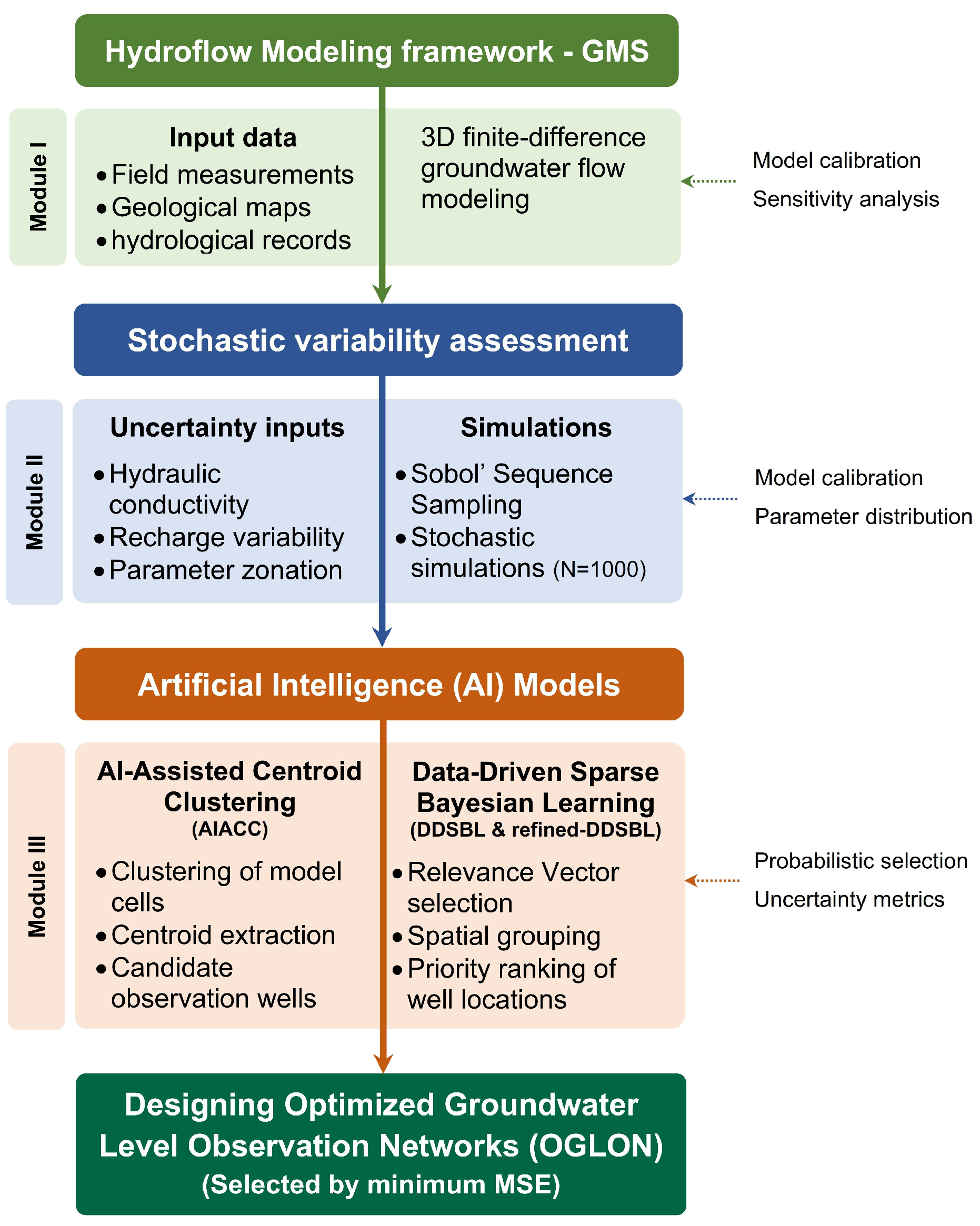
This section presents the conceptual structure of the proposed methodology, which encompasses three main stages for designing an Optimized Groundwater Level Observation Network (OGLON) (Figure 1).

Figure 1. Flowchart of the AI-integrated framework for designing Optimized Groundwater Level Observation Networks (OGLON).

Module I involves the collection of extensive environmental and subsurface information, including lithological characteristics, aquifer properties, and external forcing factors. This information is utilized to construct a numerical subsurface water system and to characterize the spatial and temporal behavior of subsurface hydrodynamics across the region under investigation.

Within Module II, probabilistic simulation techniques serve to assess and measure uncertainties associated with the groundwater model.

Module III is dedicated to determining the optimal configuration of observation wells. The quantity and spatial placement of observation points are determined through the application of a pair of advanced artificial intelligence techniques, enabling accurate prediction of hydraulic levels at each location: AI-Assisted Centroid Clustering (AIACC) and Data-Driven Sparse Bayesian Learning (DDSBL).

For each potential OGLON configuration, a corresponding GMS model is created under identical conditions, differing only in the arrangement of observation wells [42]. To execute these GMS simulations, observed hydraulic head values must be assigned to all observation wells. Accordingly, a spatially continuous surface of hydraulic levels, derived from the current measurement network, is utilized to infer representative water-level values at the locations of the newly designated observation points.

Finally, the designated network configurations are compared based on their Mean Squared Error (MSE) between interpolated (assumed observed) and simulated head values [42,43,44]. The configuration that yields the smallest MSE is identified as the optimal OGLON design.

Model validation was performed using k-fold cross-validation applied to the ensemble of stochastic groundwater simulations. The full dataset generated from the probabilistic model runs was partitioned into k mutually exclusive subsets, with k−1 folds used for training the AI models (AIACC and DDSBL) and the remaining fold used for validation. This process was repeated k times to ensure that each subset served once as an independent validation set. This strategy allowed evaluation of model generalization without requiring an external observational dataset, which is not available at the spatial resolution of the OGLON framework. The cross-validated errors were averaged across all folds and used as the primary metric to assess predictive reliability and stability of the machine-learning-based OGLON design.

2.1. Module I: Hydroflow Modeling Framework–GMS

A conceptual representation of subsurface hydrodynamics serves as the foundation for any comprehensive groundwater resource assessment. It provides an interpretive framework for understanding how groundwater moves through the aquifer system, delineating the direction of flow, identifying discharge zones, and characterizing the vertical extent and variability of the unsaturated zone. Such a model helps visualize the interaction between recharge, flow, and discharge processes and forms the basis for quantitative numerical simulations [42,43,44].

In Module I, a detailed Groundwater Simulation Framework was established using a three-dimensional finite-difference modeling approach [43,44]. This system, built within a numerical modeling environment, allows for the simulation of groundwater flow in the saturated zone and captures spatial variations in hydrogeological conditions. The study area was systematically divided into a mesh of discrete computational cells, each representing a control volume through which flow equations are solved iteratively. The grid design considered local hydrostratigraphy, aquifer thickness, and hydraulic gradients to ensure that physical processes were represented with high spatial accuracy [42,43,44].

Boundary conditions, such as constant head, no-flow, and flux boundaries, were carefully defined to reproduce the real hydrological behavior of the system. Recharge zones, rivers, wells, and discharge boundaries were all explicitly represented to reflect natural and anthropogenic influences on the aquifer. Input data included field measurements, geological maps, borehole logs, and hydrological records, which together provided the physical and hydraulic parameters necessary for simulation (e.g., hydraulic conductivity, specific yield, and porosity) [43].

The model calibration process was a crucial step aimed at minimizing the discrepancies between simulated and observed groundwater levels. Calibration was performed through iterative parameter adjustments to achieve the best statistical fit between model outputs and measured field data. Hydraulic head observations from monitoring wells across the study area were used as reference points. Sensitivity analyses were also carried out to identify the most influential parameters affecting model performance [44].

Through this systematic approach, the resulting calibrated model provides a robust and realistic depiction of groundwater flow within the study region, enabling reliable assessment of aquifer behavior, water balance estimation, and support for subsequent optimization and decision-making processes.

2.2. Module II: Stochastic Variability Assessment

In this study, stochastic simulations are employed to represent the inherent variability and uncertainty of hydrogeological parameters, including hydraulic conductivity K and recharge rate R. The simulations are conducted in the Groundwater Modeling System (GMS) using a parameter zonation approach combined with Sobol’ Sequence Sampling (Sobol Sampling) [45,46]. This quasi-random sampling method systematically fills the multidimensional parameter space, ensuring uniform coverage of each input variable and efficiently capturing its probability distribution.

Each uncertain parameter X_i (i = 1, 2,…, n) is defined by its mean μ_i, standard deviation σ_i, and upper and lower bounds [X_imin, X_imax]. Sobol Sampling generates N realizations for each parameter such that the cumulative distribution function Fx_i(y) is uniformly sampled in the interval [0, 1] (Equation (1)):

$$x_i^{\left(j\right)}=F_{X_i\left(s_i^{\left(j\right)}\right)}^{-1}, j=1, 2,\dots , N$$

(1)

where s_i^(j) is the j-th element of the Sobol sequence for variable X_i, and Fx_i⁻¹ is the inverse cumulative distribution function of X_i. This ensures that all portions of each variable’s distribution are explored, providing robust coverage of the parameter space.

To quantify model uncertainties, a total of N = 1000 stochastic simulations were performed, representing equally plausible realizations of the aquifer system. The main sources of uncertainty are limited field measurements and variability in K and R. For every simulation instance, the full span of each parameter is partitioned into N discrete segments with uniform likelihood, from which a Sobol sequence systematically extracts a representative value for each segment. The generated values for all variables are then systematically combined to form a complete set of N unique parameter vectors (Equation (2)):

$$X^{\left(j\right)}=\left(x_1^{\left(j\right)},x_2^{\left(j\right)},\cdots ,x_n^{\left(j\right)}\right), j=1, 2,\dots , N$$

(2)

Each parameter vector X^(j) is used as input to the groundwater flow model, producing a corresponding simulated hydraulic head distribution h^(j). The stochastic ensemble {h⁽¹⁾, h⁽²⁾, …, h^(N)} provides probabilistic predictions of groundwater flow and forms the training dataset for subsequent machine learning algorithms.

The variability of simulated outputs can be quantified by the ensemble mean and variance (Equation (3)):

$$\overline{h}={\displaystyle \frac{1}{N}}{\sum }_{j=1}^N{h}^{\left(j\right)}, {\sigma }_h^2={\displaystyle \frac{1}{N-1}}{\sum }_{j=1}^N{\left(h^{\left(j\right)}-\overline{h}\right)}^2$$

(3)

These statistical metrics allow identification of regions with high uncertainty, guide further data collection, and support the design of optimized groundwater observation networks [45,46].

2.3. Module III: Artificial Intelligence (AI) Models

As this study involves the development of the first-ever OGLON (optimized groundwater level observation network), a theoretically perfect scenario would assume that every grid cell within the groundwater model could serve as a potential site for an observation well. Such an exhaustive configuration would ensure complete spatial coverage of the study area, offering highly detailed insights into groundwater head variations across numerous locations. However, this approach is neither practical nor efficient for regional-scale groundwater assessments, primarily due to financial constraints.

Even in the absence of budgetary limitations, observation wells must be strategically positioned at representative sites defined by the hydrogeological characteristics of the region to minimize redundant data collection. The essence of an optimized OGLON design lies in selecting a limited yet effective number of well locations that yield accurate, distinct, and meaningful groundwater head measurements.

Accordingly, the placement of all potential wells is determined with precision to achieve comprehensive spatial representation using machine learning algorithms such as clustering and regression. This study applies two advanced techniques: AI-Assisted Centroid Clustering (AIACC) and Data-Driven Sparse Bayesian Learning (DDSBL) and performs a comparative evaluation of the outcomes produced by each method [35,36,37,38,39,40,41].

In addition, a refined group of candidate wells identified through the DDSBL technique is chosen as the optimal set of observation wells and subsequently evaluated against other OGLON configurations [38,39,40,41]. The machine learning models are trained using a suite of parameters derived from the groundwater model, which encompass each cell’s geographic coordinates (longitude and latitude), upper and lower elevation limits, mean groundwater head, and its variability as determined through stochastic simulations. Additional input variables include hydraulic conductivity, recharge intensity, and evapotranspiration rate [38,39,40,41].

Cells corresponding to river channels, sewer networks, or those that have experienced desiccation in one or more stochastic realizations are systematically excluded from the dataset. This filtering step ensures that the algorithms do not misinterpret such cells as viable monitoring sites, thereby improving the reliability and physical relevance of the optimized network design.

2.4. Computational Requirements

In terms of data volume, the workflow relies on a large ensemble of hydrogeological realizations and spatially distributed model outputs. A total of 1000 stochastic groundwater simulations were generated, each producing full 3D hydraulic-head fields across all model cells. This resulted in approximately 2.5–3 million training records for the ML algorithms. The computational requirements are substantial: simulations were executed on a workstation. The full set of stochastic simulations required roughly 18–22 h, while preprocessing and ML training (AIACC and DDSBL) required an additional 2–3 h. Once trained, however, both algorithms run efficiently and can be executed on standard desktop computers without high-performance computing resources. The generalization potential of the framework is high because all required model inputs; hydraulic heads, hydrostratigraphic parameters, recharge, topography, and their stochastic ranges, are commonly available in most regional groundwater studies. The methodology does not depend on site-specific empirical tuning, enabling straightforward transferability to other basins with different environmental or geological settings, provided that a calibrated numerical model and basic hydrogeological datasets are available.

3. AI-Integrated Models for Designing OGLON

3.1. Unsupervised Clustering: AI-Assisted Centroid Clustering (AIACC)

The AI-Assisted Centroid Clustering (AIACC) technique represents an advanced data-partitioning algorithm designed to segment a dataset into distinct centroid-based groups. Within hydrogeological modeling, this approach enables the systematic classification of groundwater model cells into spatially coherent clusters, facilitating the identification of the most representative locations for the installation of observation wells within an Optimized Groundwater Level Observation Network (OGLON) [35,36,37].

The AIACC method seeks to minimize the total intra-cluster variance (or within-cluster sum of squares), expressed as Equation (4):

$$J=\sum _{i=1}^K\sum _{x_j\in C_i}{‖x_j-{\mu }_i‖}^2$$

(4)

where K indicates the total cluster count, C_i defines the collection of elements (model cells) allocated to cluster i, x_j corresponds to the feature vector of a specific model cell (including parameters such as hydraulic conductivity, recharge, and groundwater level), and μ_i is the centroid of cluster i, computed as the mean of all data points within C_i (Equation (5)):

$${\mu }_i={\displaystyle \frac{1}{\left|C_i\right|}}\sum _{x_j\in C_i}{x}_j$$

(5)

The clustering process iteratively refines centroid positions until convergence, defined when the change in the objective function J between iterations falls below a specified threshold ϵ (Equation (6)):

$$\left|J_{t+1}-J_t\right|<ϵ$$

(6)

To identify the most appropriate number of clusters K, AIACC employs model selection techniques such as the Elbow Method, which examines the inflection point of the variance-reduction curve, or the Silhouette Coefficient, given by Equation (7) [47]:

$$S\left(i\right)={\displaystyle \frac{b\left(i\right)-a\left(i\right)}{max\left\{a\left(i\right), b\left(i\right)\right\}}}$$

(7)

where a(i) is the mean intra-cluster distance for cell i, and b(i) is the minimum mean distance from i to any other cluster.

Upon convergence, each cluster centroid μ_i signifies the optimal representative of its spatial domain. The model cell whose coordinates are nearest to this centroid, according to the Euclidean distance d(x_j,μ_i) = ǁx_j − μ_iǁ, is selected as the candidate site for an observation well [47], ensuring efficient spatial coverage and minimal data redundancy within the designed OGLON.

3.2. Supervised Clustering: Data-Driven Sparse Bayesian Learning (DDSBL)

The Data-Driven Sparse Bayesian Learning (DDSBL) approach represents a probabilistic and data-adaptive framework designed to generate sparse and interpretable solutions for regression and classification problems. It is fundamentally grounded in Bayesian inference, which estimates posterior distributions over model parameters while promoting sparsity through hierarchical priors [38,39,40,41].

The DDSBL algorithm is calibrated using a collection of paired observations (X,y), where each instance comprises a set of predictor variables and its corresponding response. The predictor matrix, expressed as X = [x₁, x₂, …, x_N]^T contains all feature vectors, while the associated response vector y = [y₁, y₂, …, y_N]^T holds the observed outcomes for each instance. Within this framework, the model posits a linear relationship between inputs and outputs, incorporating Gaussian-distributed residuals to account for measurement noise and unmodeled variability Equation (8):

$$y=Xw+ϵ$$

(8)

where w is the vector of model weights, ε is the noise term assumed to follow a Gaussian distribution N(0,σ²I).

To enforce sparsity, DDSBL assigns an independent Gaussian prior to each weight ((Equation (9)):

$$p\left(w|\alpha \right)=\prod _{i=1}^{M}N\left(w_i|{0,\alpha }_i^{-1}\right)$$

(9)

where α = [α₁, α₂, ..., α_M] are precision hyperparameters governing the relevance of each input feature. The posterior distribution of the weights, conditioned on the data, is derived using Bayes’ theorem shown in Equation (10):

$$p\left(w|X,y,\alpha ,{\sigma }^2\right)={\displaystyle \frac{p\left(y|X,w,{\sigma }^2\right)p\left(w|\alpha \right)}{p\left(y|X,\alpha ,{\sigma }^2\right)}}$$

(10)

In hydrogeological applications, the DDSBL model is provided with input features that include the geographic coordinates (X and Y position) along with the mean hydraulic levels calculated for every computational grid. The output variable represents the variability of hydraulic levels obtained from probabilistic simulations [38,39,40,41].

The algorithm iteratively updates the hyperparameters α and the noise variance σ² to maximize the marginal likelihood, leading to the automatic pruning of irrelevant components, those with large α_i values, thus identifying only the most influential data points. These influential points are termed Relevance Vectors, which serve as the backbone of the sparse model representation.

After each run of DDSBL, the method yields the spatial distribution and count of Relevance Vectors, highlighting the most significant cells influencing groundwater variability. Repeating the algorithm multiple times ensures consistency and robustness in the selection of these key points.

Once the ensemble of Relevance Vectors is obtained, they are spatially grouped based on mutual proximity using a clustering distance criterion d_ij (Equation (11)):

$$d_{ij}=‖r_i-r_j‖$$

(11)

where r_i and r_j represent the coordinates of two Relevance Vectors. For each cluster, the local density ρ_k is computed as Equation (12):

$${\rho }_k={\displaystyle \frac{n_k}{A_k}}$$

(12)

where n_k is the number of Relevance Vectors within cluster k, and A_k is its spatial area. The relative occurrence probability for each cluster is then expressed as Equation (13):

$$P_k={\displaystyle \frac{{\rho }_k}{\sum _{j=1}^K{\rho }_j}}$$

(13)

Each cluster’s centroid, representing the spatial mean of its Relevance Vectors, is interpreted as a potential location for an observation well within the OGLON framework. The corresponding probability P_k quantifies the likelihood or priority of installation at that site, allowing decision-makers to rank observation well locations based on available financial resources and monitoring objectives.

In this study, significant Relevance Vectors were identified through the Sparse Bayesian Learning (SBL) mechanism embedded in DDSBL. Each weight w_i is governed by a precision hyperparameter α_i, updated via maximum likelihood (evidence maximization) (Equations (10) and (11)). During iteration, inputs whose α_i values consistently increase contribute minimally to the posterior and are pruned, whereas Relevance Vectors correspond to parameters for which α_i converges to stable, finite values. This hyperparameter–driven pruning criterion is the basis for selecting statistically influential Relevance Vector points within the DDSBL framework.

3.3. Supervised Clustering: Refined Data-Driven Sparse Bayesian Learning (Refined-DDSBL)

The Refined Data-Driven Sparse Bayesian Learning (Refined-DDSBL) enhances DDSBL by integrating statistical refinement and spatial clustering of Relevance Vectors to improve the design of Optimized Groundwater Level Observation Networks (OGLON). After multiple DDSBL runs, each Relevance Vector r_i is assigned an occurrence frequency f_i, defined as the number of times r_i is selected divided by the total number of iterations N_run as Equation (14):

$$f_i={\displaystyle \frac{n_i}{N_{run}}}$$

(14)

Only Relevance Vectors exceeding a predefined threshold fth are retained. These high-probability Relevance Vectors are then spatially grouped using Euclidean distance as Equation (11).

For each cluster C_k, the local density ρ_k and relative occurrence probability P_k are computed as Equations (12) and (13).

Where n_k is the number of Relevance Vectors in the cluster and A_k its spatial area. The cluster centroid μ_k, representing the mean coordinates of Relevance Vectors in C_k, is interpreted as a candidate observation well location as Equation (15):

$${\mu }_k={\displaystyle \frac{1}{n_k}}\sum _{r_i\in C_k}{r}_i$$

(15)

Clusters with higher P_k values are prioritized, ensuring that selected wells maximize spatial coverage, minimize redundancy, and capture the most influential hydrogeological variability for OGLON.

4. Study Area

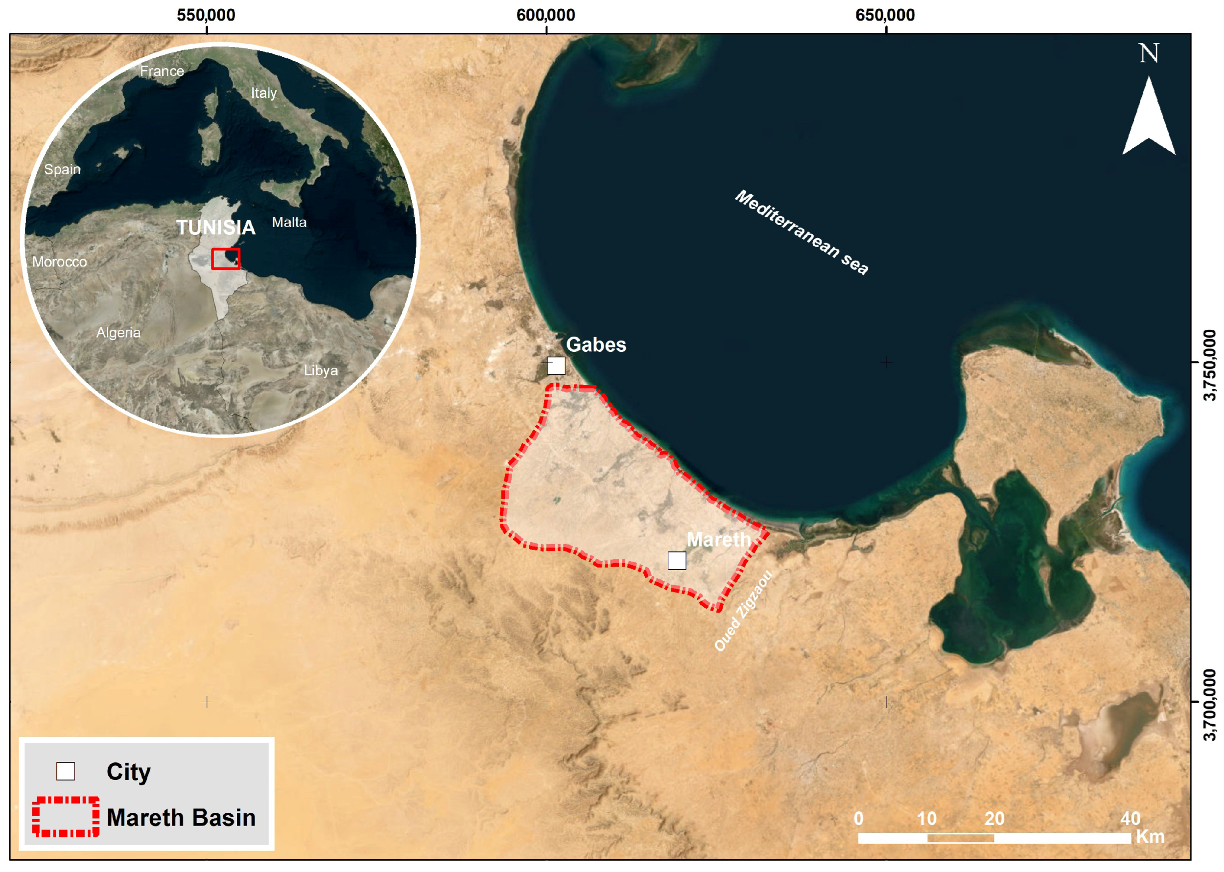
The Mareth Basin, located in the southeastern region of Tunisia, constitutes part of the extensive Djeffara depression, a wide sedimentary structure stretching from the Gabès plain northward to Oued Zigzaou in the south (Figure 2). Lying directly along the Mediterranean shoreline, this area holds a prominent hydrogeological and economic role in southern Tunisia, where agricultural and human activities are particularly concentrated.

Figure 2. Study area.

The basin falls within an arid to hyper-arid zone, typified by low and highly variable rainfall averaging about 162 mm annually. Roughly four-fifths of total precipitation occur from September through March, followed by a long dry interval between April and September [48]. The mean annual temperature fluctuates between 19 °C and 22 °C, occasionally rising well above these values in summer [48]. The potential evapotranspiration (PET), estimated at more than 1000 mm yr⁻¹, greatly surpasses precipitation inputs and leads to a persistent climatic water imbalance [48,49]. In contrast, actual evapotranspiration (AET) averages 178 mm yr⁻¹, and infiltration rates rarely exceed 45 mm yr⁻¹, demonstrating the limited recharge potential of the system under present-day climatic constraints [48,49,50].

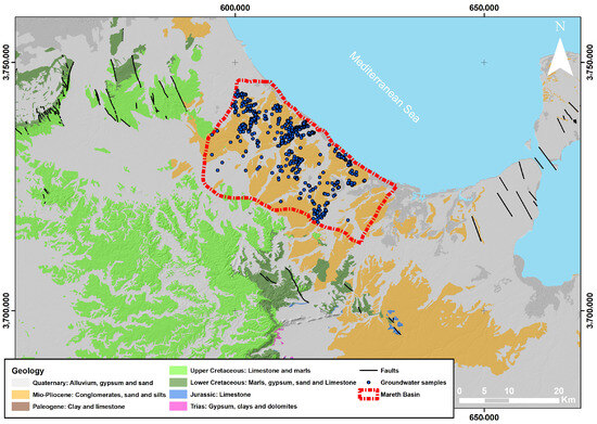
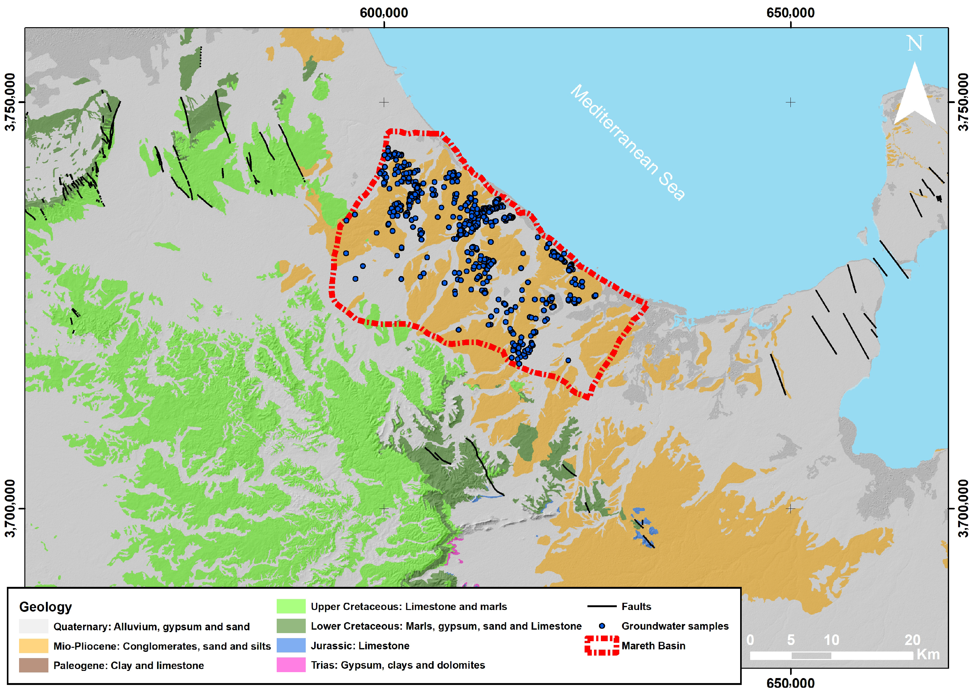
The tectono-sedimentary evolution of the Mareth depression has been shaped by repeated extensional movements and subsidence modules, which fragmented the basin through numerous normal faults. These structures dictate both the lithostratigraphic framework and the directions of groundwater circulation [48,49,50,51,52,53]. The stratigraphic succession, spanning from the Jurassic to the Cenozoic, is composed of heterogeneous deposits of sands, sandy clays, conglomerates, limestones, dolomites, evaporites (halite and gypsum), and carbonate facies (Figure 3) [48,51,52,53,54].

Figure 3. Geological map of the Mareth basin.

Such lithological complexity reflects the alternation of continental, fluvial, and shallow-marine depositional environments, resulting in aquifers with contrasting hydraulic characteristics and non-uniform flow dynamics. The upper formations, particularly those rich in evaporites and carbonates, exert substantial control over groundwater chemistry, explaining the spatial heterogeneity of salinity and mineralization observed throughout the basin [48,51,52,54].

From a hydrogeological perspective, the system consists of multiple aquifer layers, of which the Mio-Plio-Quaternary unit represents the main phreatic reservoir [51,54]. This aquifer exhibits notable transmissivity, with hydraulic conductivity (K) reaching up to 60 m·day⁻¹. The piezometric head (h) varies widely, ranging from approximately 2 m near coastal outlets to 50 m in the interior recharge zones [48,51,54,55]. Groundwater generally flows westward to eastward, ultimately discharging into the Mediterranean Sea. However, this natural flow regime has been severely modified by excessive abstraction, resulting in progressive water-level decline and an increasing risk of seawater intrusion where pumping exceeds recharge [48,50,54,55].

Groundwater dynamics in the Mareth Basin have undergone substantial alteration over the past decades due to intensive abstraction from wells and boreholes, primarily for irrigated agriculture. The expansion of oasis-based systems and open-field farming, dominated by date palms, cereals, and vegetables, has caused a continuous drop in groundwater levels, particularly in areas of concentrated pumping [50,54,55].

Long-term piezometric monitoring reveals a steady decline of 0.5 to 1.2 m per year in several sectors, with the most pronounced drawdowns recorded in the central and coastal parts of the basin, where the aquifer is heavily solicited. This persistent depletion of the water table reflects an imbalance between abstraction and natural recharge, aggravated by reduced rainfall and increased evapotranspiration [48,49,50,54].

As a result, several springs and shallow wells have dried up, while hydraulic gradients have shifted toward the inland, promoting seawater intrusion in low-lying zones and altering the hydraulic equilibrium of the system. In many pumping fields, piezometric depressions (cones of depression) have expanded and merged, indicating regional-scale overexploitation [50,54,55].

If current abstraction rates persist, further drawdown and salinization risks are expected, threatening the sustainability of agricultural production and the long-term viability of the phreatic aquifer.

To analyze the spatial and temporal evolution of groundwater levels, a network of 565 observation wells and production boreholes was systematically monitored across the Mareth Basin between February and May 2025. Water-level measurements were conducted using automatic piezometric loggers and manual depth-to-water recordings, ensuring high temporal resolution and spatial coverage [48,49,50,54].

The resulting data were integrated into a georeferenced database to produce piezometric contour maps, highlighting major recharge and discharge zones as well as depression cones associated with overexploited areas. These maps reveal clear SW–NE flow patterns with localized anomalies corresponding to regions of intense abstraction near agricultural perimeters and coastal zones [50,54,55].

Time-series analysis indicates a progressive lowering of the piezometric surface, consistent with declining recharge and increasing pumping intensity. The 2025 campaign provides a baseline reference for evaluating the future evolution of groundwater reserves and for implementing sustainable water management strategies within the basin.

5. Results

This section presents the outcomes derived from the simulation of groundwater dynamics, probabilistic modeling, and the formulation of the OGLON framework through classification and predictive modeling techniques. The subsurface hydrodynamic simulations and probabilistic analyses serve as foundational datasets for machine learning algorithms utilized in the OGLON development across the study region. Additionally, this section details the modeling outputs related to both the current observation wells and the newly proposed OGLON configurations.

5.1. Groundwater Dynamics (Current Monitoring Wells)

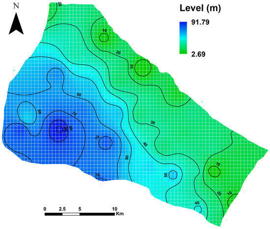
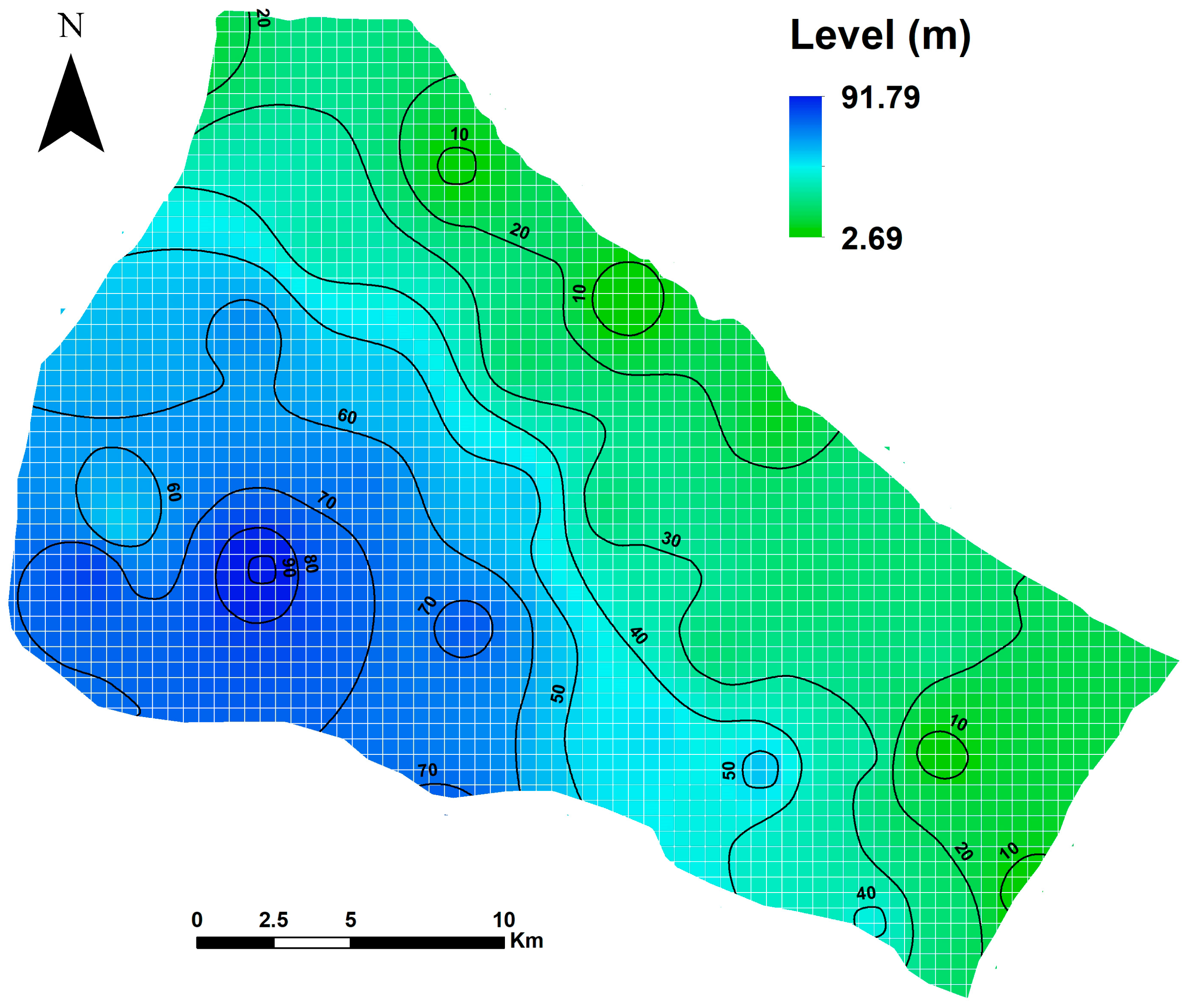
The preliminary simulation of subsurface water circulation reveals a dominant flow trend extending from the southwest toward the northeast within the Mareth basin, ultimately discharging into the Mediterranean Sea (Figure 4). While localized variations in flow direction may occur, the current assessment concentrates on regional-scale groundwater behavior. The aquifer displays lower water levels in the east-northeast, consistent with findings from field surveys and prior research, whereas in the western sector, groundwater lies at greater depths associated with higher terrain elevations.

Figure 4. Preliminary groundwater level and flow direction results from GMS.

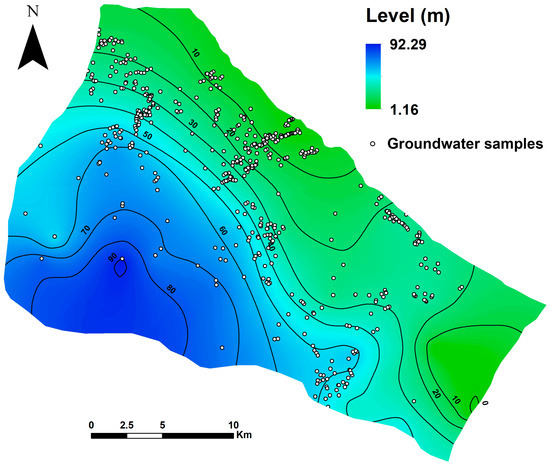
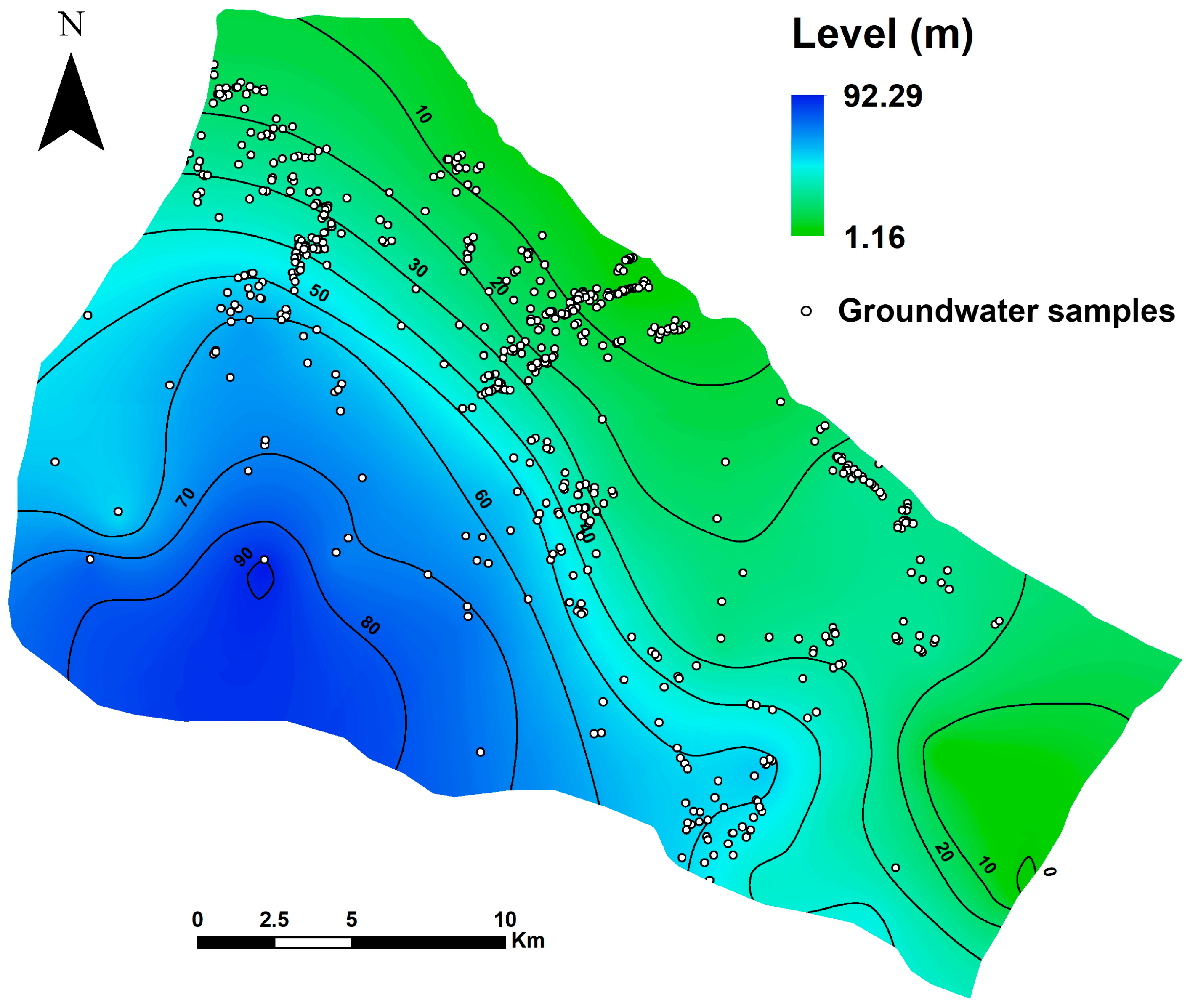
Despite the limited availability of groundwater monitoring data, the model was refined to the highest achievable accuracy using an automated parameter optimization procedure to adjust hydraulic conductivity and recharge rates. The calibration process relied on groundwater head measurements recorded between February and May 2025 across 565 monitoring wells within the study region. The finalized groundwater flow simulation (Figure 5) incorporates these wells and demonstrates that the overall flow pattern remains consistent with the preliminary findings. Nevertheless, distinct flow variations emerge in the central and southern parts of the basin, where groundwater movement appears more uniform. The calibrated simulation also indicates that groundwater levels range approximately from 1.00 m to 92.00 m, compared to an initial range of about 2.00 m to 91.00 m in the preliminary model.

Figure 5. Groundwater level and flow model calibration in GMS (February–May 2025).

5.2. AI-Assisted Centroid Clustering (AIACC) Algorithm

Because it is not feasible to install groundwater monitoring wells in every computational grid of the model, grouping the hydrogeological attributes of the study region provides an effective way to minimize and optimize he density of monitoring sites required within the OGLON system. To achieve this, an AI-Assisted Centroid Clustering (AIACC) approach was employed to categorize all model cells according to their hydrogeological properties and the variability of subsurface water table levels obtained from probabilistic modeling.

To identify the optimal cluster count for the AIACC method, cluster validity metrics such as the Elbow criterion and Silhouette coefficient were employed. Considering the hydrogeological behavior of the Mareth basin, the clustering process was set to 30 groups, as this configuration yielded the first and highest Silhouette score.

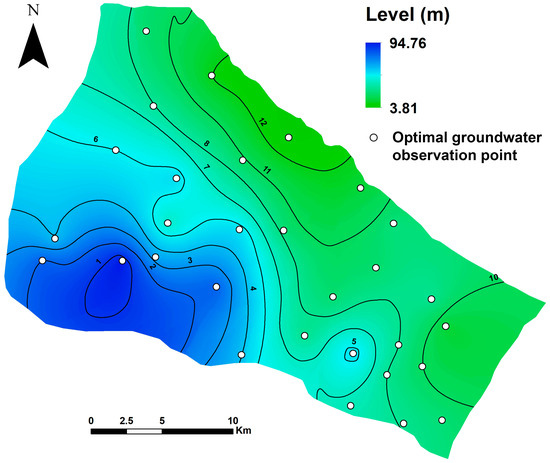
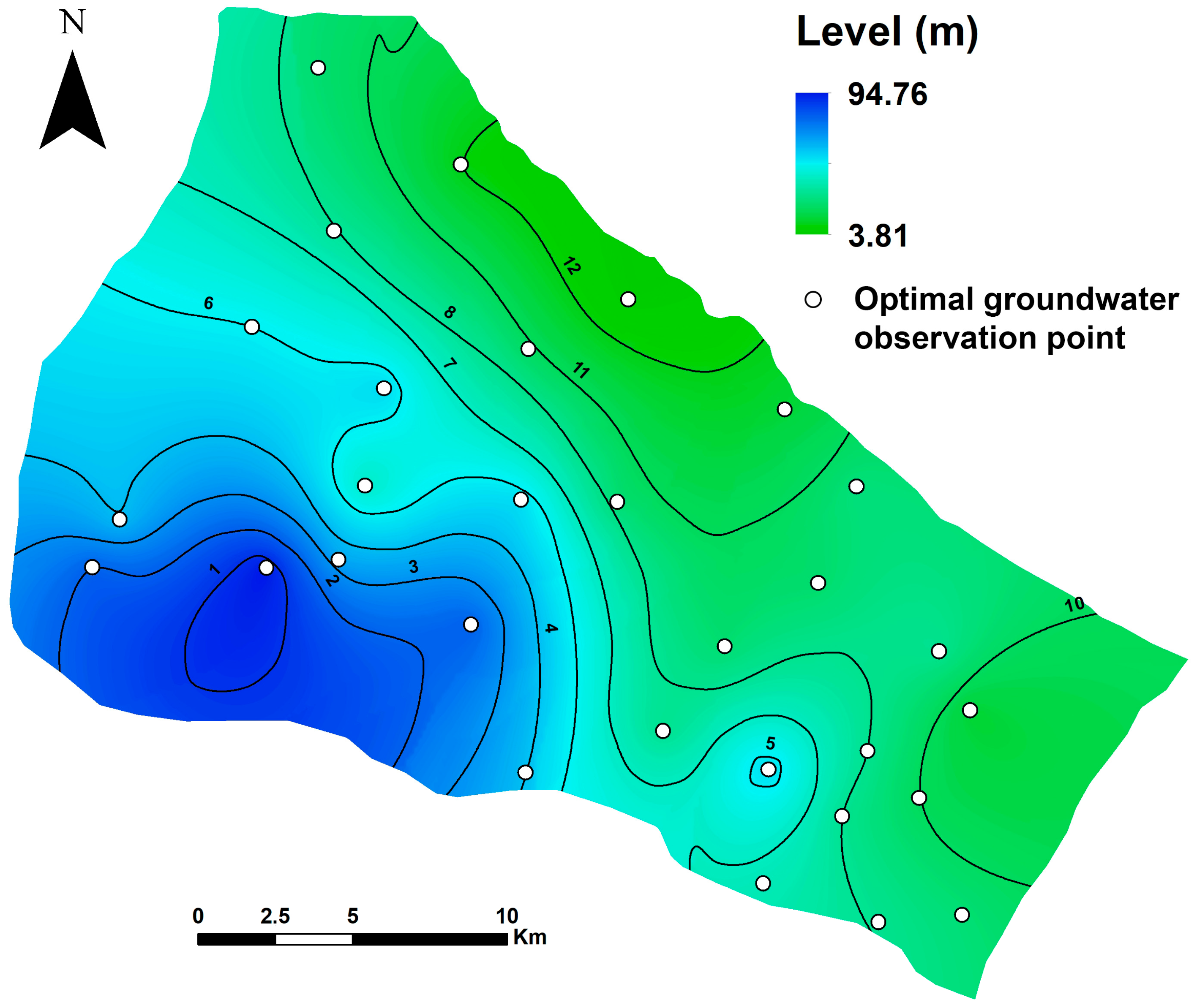
As outlined in the methodological framework, the centroid locations identified through the AIACC process were integrated into the initial groundwater model as virtual observation points. To assess the performance of the AIACC-based OGLON, groundwater head data recorded between February and May 2025 were interpolated at these centroid positions. The calibrated simulation of the OGLON developed using the AIACC procedure (Figure 6) indicates groundwater levels ranging approximately from 3.00 m to 94.00 m, averaging around 49.28 m, which is lower than the calibrated head levels shown in Figure 5. The overall flow direction remains consistent with the previous calibrated model, though variations in the central and southern zones are comparatively minor. Furthermore, the model’s initial error value of 17,232 was substantially reduced to 31.30 following the calibration process.

Figure 6. AIACC-based design of the OGLON for groundwater level and flow modeling.

5.3. Data-Driven Sparse Bayesian Learning (DDSBL) Method

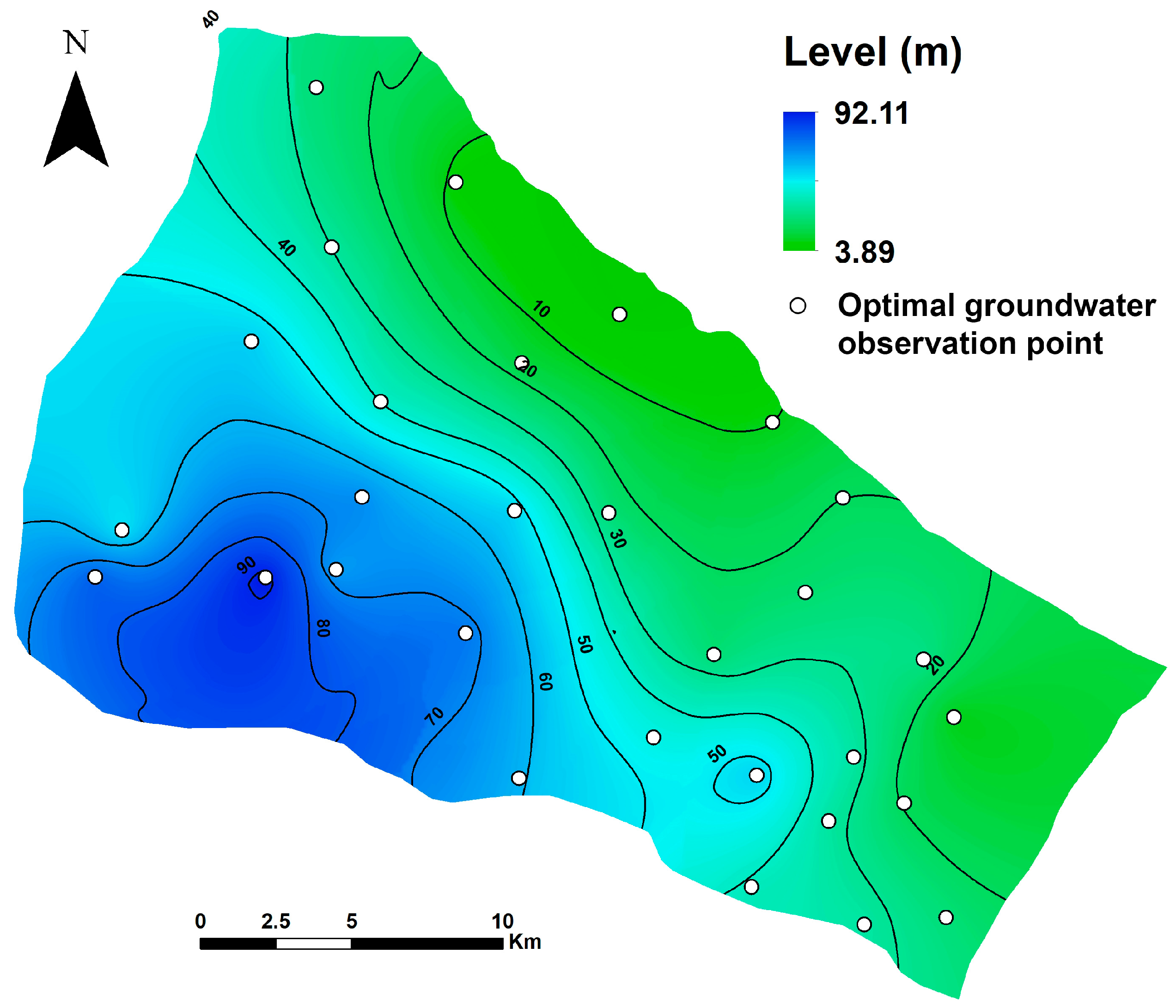
The Data-Driven Sparse Bayesian Learning (DDSBL) method was employed to construct an optimized layout for the OGLON, integrating machine learning principles with probabilistic modeling to determine the most effective monitoring locations. The resulting analysis (Figure 7) illustrates the spatial distribution of the Relevance Vectors generated throughout multiple DDSBL training cycles. Although the training samples were independently drawn from stochastic groundwater simulations, the algorithm consistently converged on similar spatial nodes, highlighting their statistical significance in representing regional hydrogeological behavior. To refine the configuration, the identified Relevance Vectors were partitioned into 30 distinct groups, and the geometric center of each group was designated as the optimal position for establishing monitoring wells within the proposed observation network.

Figure 7. DDSBL-based design of the OGLON for groundwater level and flow modeling.

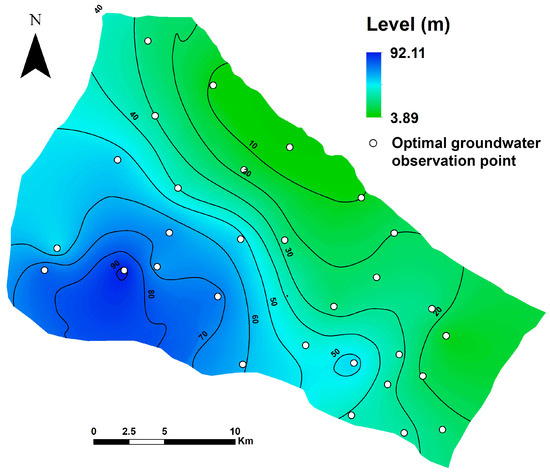
Adopting a procedure analogous to the AIACC method, the centroids derived from the DDSBL clustering are treated as the observation points for the OGLON and integrated into the groundwater model. The GMS simulation was executed using these newly proposed monitoring wells, producing the groundwater head distribution presented in Figure 7. Results indicate water levels ranging approximately from 3.00 m to 92.00 m, with the overall flow pattern largely consistent with previous models, except for minor localized variations. The inclusion of additional observation wells initially increased the model error to 25,968, which was substantially reduced to 1103 following the calibration process.

5.4. Refined-DDSBL Algorithm

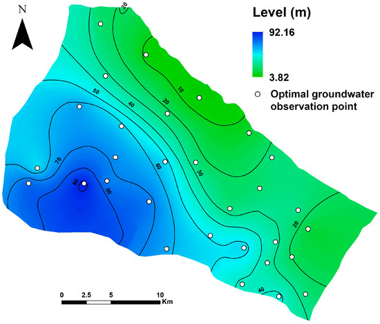
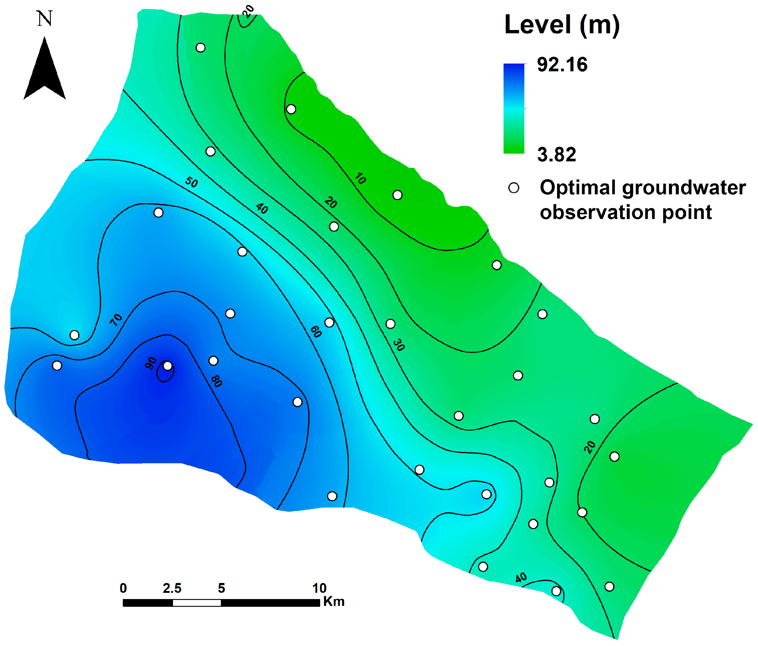
Because the DDSBL-based OGLON still exhibited a relatively high model error, the network was refined by selecting the 30 observation wells corresponding to the highest occurrence probability of Relevance Vectors. The calibrated groundwater simulation incorporating these wells is presented in Figure 8. The results reveal groundwater levels ranging from approximately 3.00 m in the northeast to 92.00 m in the western part of the study area. While the preliminary simulation discrepancy was 21,355 as a result of the increased density of monitoring locations, calibration successfully reduced it to 1.32, demonstrating a significant improvement in model performance.

Figure 8. Refined-DDSBL-based design of the OGLON for groundwater level and flow modeling.

5.5. Sensitivity Analysis of Stochastic Simulations

Uncertainty associated with the stochastic groundwater simulations was assessed through an ensemble-based analysis carried out over 1000 Monte Carlo realizations of hydraulic conductivity and recharge. For each parameter, the spatial variance and coefficient of variation in simulated hydraulic heads were computed across all realizations to quantify the magnitude and spatial distribution of predictive uncertainty. Results indicate that the highest uncertainty occurs in the central and southeastern sectors of the basin, where observation data are sparse and hydrostratigraphic heterogeneity is greatest.

To complement this assessment, a sensitivity analysis was performed using variance-based indices derived from the ensemble. Hydraulic conductivity exhibited the highest first-order sensitivity across most of the domain, followed by recharge, confirming their dominant influence on simulated water levels. Areas with elevated sensitivity coincide with zones where the optimized OGLON designs (AIACC and Refined-DDSBL) place additional wells, demonstrating the effectiveness of these networks in targeting regions where model outputs are most responsive to parameter perturbations.

This combined uncertainty–sensitivity evaluation supports the interpretation of the stochastic modeling results and justifies the spatial distribution of monitoring wells proposed in the optimized networks.

5.6. Uncertainty Evaluation

In the Mareth basin, existing monitoring wells are irregularly distributed and record groundwater data only at sporadic intervals, resulting in gaps in hydrogeological information. Both the AI-Assisted Centroid Clustering (AIACC) and Data-Driven Sparse Bayesian Learning (DDSBL) algorithms identify optimal centroids to determine the most effective locations for OGLON observation wells. By targeting areas lacking measurements, these proposed wells enhance data coverage and provide a more comprehensive understanding of regional groundwater dynamics.

In the DDSBL-based network, deploying 30 observation wells would inevitably raise the total costs for OGLON implementation, including installation, data acquisition, and long-term maintenance. The performance of the groundwater model using existing wells and the proposed OGLON is summarized in Table 1. Analysis of the results shows that the model incorporating the AIACC-designed network produces fewer errors compared to both the current observation wells and the DDSBL network. Moreover, despite its comprehensive coverage, the DDSBL network exhibits the highest model errors, making it less favorable for OGLON design in its original form.

Table 1. Evaluation of groundwater prediction accuracy using different configurations of OGLON.

Metric	Current Monitoring Wells	AI-Assisted Centroid Clustering (AIACC)	Data-Driven Sparse Bayesian Learning (DDSBL)	Refined-DDSBL
ME	−0.0512	0.0328	−0.0457	0.0054
MAE	0.3125	0.1279	0.4213	0.0091
RMSE	0.5028	0.2145	0.6678	0.0153

To improve its performance and enable a fair comparison with the AIACC network, the DDSBL network was refined by selecting 30 wells corresponding to the highest Relevance Vector frequencies. The model calibrated with this refined DDSBL network demonstrates the lowest error among all configurations, indicating that this approach provides the most effective and reliable design for an OGLON.

Groundwater modeling inaccuracies stem from simplifications in the conceptual framework and uncertainties in input variables, reflecting the divergence between computed outputs and measured field observations. Throughout the calibration phase, these uncertain variables are iteratively refined to reduce discrepancies and enhance model fidelity. During calibration, these uncertain parameters are systematically adjusted to minimize the model error.

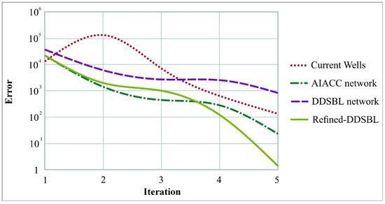
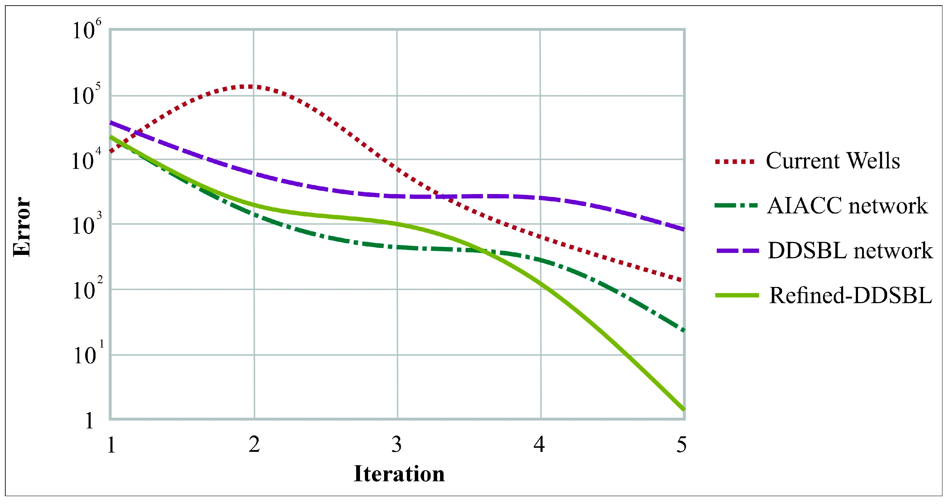
Figure 9 highlights how the calibration error evolves under each OGLON configuration and demonstrates the contrasting performance of the four networks. The “Current Wells” scenario shows the slowest and least stable reduction in error, with a noticeable rise during the second iteration, indicating the influence of uneven spatial coverage and redundant wells on model convergence. The AIACC network exhibits a more consistent decrease in error across iterations, reflecting the benefits of improved spatial clustering. The DDSBL configuration achieves a faster initial error reduction but stabilizes at a higher residual error compared to the refined approach. In contrast, the Refined-DDSBL network delivers the most efficient calibration behavior, with a sharp and continuous decline in error from iteration 1 to iteration 5, ultimately achieving the lowest final error among all scenarios. This confirms its superior capability to retain the most informative wells and guide the model toward a more stable and accurate solution.

Figure 9. Convergence behavior of model error for different OGLON configurations.

As discussed in the previous section, all modeled scenarios display a consistent regional groundwater flow pattern, with minor variations observed at specific localities, aligning well with prior studies on the hydrogeology of the Mareth basin. Groundwater predominantly moves from the northeast toward the southeast, ultimately discharging into the Mediterranean Sea. A comparison of the simulated head levels across the different model configurations is presented in Table 2.

Table 2. Variations in groundwater levels within current monitoring wells and proposed OGLONs.

Parameter	Current Monitoring Wells	AI-Assisted Centroid Clustering (AIACC)	Data-Driven Sparse Bayesian Learning (DDSBL)	Refined-DDSBL
Minimum Level (m)	1.16	3.81	3.89	3.82
Maximum Level (m)	92.29	94.76	92.11	92.16
Average Level (m)	46.72	49.28	48.00	47.99
Level Variance	2076.17	2067.98	1945.69	1950.99
Max. Level–Min. Level (m)	91.13	90.95	88.22	88.34
70th Percentile of Levels	64.95	67.47	65.64	65.66
Mean Surface Altitude (m)	215	-	-	-
Mean (Surface altitude–Level) (m)	168.28	165.72	167.00	167.01

The configuration of observation wells strongly influences groundwater representation in the Mareth basin. Existing wells exhibit high variability due to irregular placement, while the AIACC network captures higher and more representative groundwater levels, effectively targeting key hydrogeological zones. The original DDSBL network provides more uniform coverage but underrepresents extreme values. Refining DDSBL to the 30 most significant wells balances uniformity and accuracy, producing results comparable to AIACC. Overall, both the AIACC and Refined-DDSBL networks improve spatial coverage and groundwater representation compared to existing wells (Table 2).

6. Discussion

The results of this study demonstrate that the configuration and density of groundwater observation networks strongly influence model performance, particularly in arid and coastal aquifers. In the Mareth basin, the existing monitoring wells are sparsely and irregularly distributed, which increases model uncertainty and limits the representation of local hydrogeological variability. Such limitations have been similarly reported in semi-arid and coastal systems worldwide, where uneven well distribution reduces the reliability of groundwater modeling and hampers decision-making for water resource management [6,7,9,10,27].

Compared with these earlier findings, the AI- and ML-based OGLON configurations developed in this study provide quantitatively stronger improvements. For example, while previous optimization studies generally report moderate reductions in prediction error, the AIACC configuration in this work reduced RMSE from 0.5028 m (existing wells) to 0.2145 m, and the refined DDSBL approach further decreased error to 0.0153 m. This magnitude of improvement is substantially higher than error reductions commonly achieved through classical geostatistical optimization or heuristic network design methods reported in coastal aquifers.

The AIACC algorithm effectively identifies hydrogeologically meaningful clusters that capture both low and high groundwater levels. This results in a more realistic representation of groundwater gradients, similar to the improvements noted in clustering-based network optimization approaches, but with a larger reduction in model error and better coverage of extreme values. The DDSBL method, rooted in Bayesian sparsity, highlights statistically influential locations in a manner consistent with earlier probabilistic optimization studies [40,41], yet the performance in this study surpasses typical outcomes because the relevance vectors were refined and integrated with stochastic groundwater simulations rather than relying solely on empirical data.

A key insight from this study is that machine learning–optimized networks do not only reduce errors; they also outperform traditional designs in capturing hydrogeological extremes, which are often overlooked in conventional observation networks. Several earlier works emphasize that high-variance zones and areas near discharge boundaries are generally poorly monitored in sparse networks [11,15,29,34]. Our results directly confirm this: both AIACC and refined DDSBL improve representation of minimum and maximum water levels (Table 2), providing a more realistic depiction of the dominant flow trend toward the Mediterranean Sea and local-scale variations in the central and southern basin.

Another important comparison with literature concerns network density and cost-effectiveness. Studies in arid and coastal environments often conclude that denser networks improve accuracy but drastically increase installation and maintenance costs [48,49,54]. The refined DDSBL network developed here contradicts this trend by achieving the lowest model error using only 30 wells, demonstrating that a fully optimized sparse network can outperform both denser AIACC configurations and existing wells. This directly supports the argument made in previous adaptive monitoring studies [43,44] that machine-learning-driven designs can reduce costs without compromising scientific rigor.

Despite these advantages, practical implementation of OGLONs may face challenges. Data availability can limit the development of a robust stochastic model, while field logistics, including accessibility, terrain constraints, and installation capacity, can influence network deployment. Long-term maintenance costs, such as sensor calibration, data acquisition, and well upkeep, must also be considered when planning optimized networks. Recognizing these constraints is essential to ensure that AI- and ML-based designs can transition from theoretical models to operational monitoring systems.

Finally, the scalability and adaptability of ML-based designs were confirmed. Similarly to previous findings that ML techniques allow iterative improvement as new data become available [35,37,47], the DDSBL framework in our study can dynamically update well significance based on additional stochastic simulations. This adaptive capability enables integration with future monitoring programs, where real-time data or periodic field campaigns can continuously refine network configuration, ensuring sustained performance as environmental conditions or hydrogeological dynamics evolve.

While the present study focuses on AIACC and DDSBL, other AI-based optimization approaches, such as Genetic Algorithms (GA), Particle Swarm Optimization (PSO), or Artificial Neural Network (ANN)-based frameworks, have also been applied to groundwater network design. The methods used here offer distinct advantages in handling stochastic simulations and spatial clustering, but future work could benchmark performance against these alternative approaches to evaluate efficiency, predictive accuracy, and adaptability across different hydrogeological contexts.

The comparison with existing literature clearly shows that the AIACC and refined DDSBL approaches not only align with but also significantly advance current methodologies for groundwater observation network optimization. They provide higher predictive accuracy, better spatial representation, and more cost-efficient configurations than traditional or previously published network designs.

To assess the robustness of the proposed OGLON configurations and mitigate overfitting risks, cross-validation was performed using independent subsets of stochastic groundwater simulations. Both AIACC and Refined-DDSBL models were trained on a portion of the data and validated on the remaining simulations to ensure consistent predictive performance. The low variance in model error across validation sets indicates that the selected observation wells capture the essential hydrogeological variability without overfitting to specific training instances. Moreover, repeating the DDSBL procedure multiple times and retaining only high-frequency Relevance Vectors further reduces the influence of outlier or spurious data points, ensuring that the refined network represents statistically significant and spatially robust monitoring locations.

Despite the promising results, this study has certain limitations. The proposed OGLON configurations were developed and tested within a single aquifer system (Mareth basin), which may limit generalizability to regions with different hydrogeological characteristics or data availability. Additionally, the current approach relies on stochastic groundwater simulations, which themselves are subject to uncertainties in input parameters and boundary conditions. Future research could explore the integration of real-time monitoring data to dynamically update the OGLON, incorporate more diverse aquifer types to validate transferability, and investigate hybrid AI/ML models combining physical process constraints with advanced clustering techniques to further enhance robustness and predictive reliability.

The proposed AI- and ML-based OGLON framework has potential applicability beyond the Mareth basin. Its modular design, combining stochastic groundwater modeling with machine learning–driven well selection, allows adaptation to other hydrogeological settings, including confined, unconfined, or multi-layered aquifers. Transferability would require adjusting input parameters to local hydrogeological properties, but the underlying methodology remains consistent. Moreover, the framework is scalable: the number of potential observation wells, spatial resolution, and stochastic simulation ensemble size can be modified to suit larger or smaller basins, or areas with denser or sparser monitoring networks. This flexibility suggests that the approach could support regional groundwater management and adaptive monitoring strategies in diverse environmental contexts, provided that baseline hydrogeological data and a calibrated numerical model are available.

7. Conclusions

This study demonstrates the effectiveness of an integrated AI- and ML-based framework for the design of Optimized Groundwater Level Observation Networks (OGLONs), applied to the Mareth Basin in southeastern Tunisia. The framework combines stochastic groundwater modeling, hydrogeological parameter variability analysis, and machine learning algorithms (AI-Assisted Centroid Clustering (AIACC) and Data-Driven Sparse Bayesian Learning (DDSBL)) to determine the most efficient density and spatial configuration of observation wells. Quantitative analyses reveal significant enhancements in network performance and model accuracy achieved through these methodologies.

The existing network of 565 observation wells exhibited a Root Mean Squared Error (RMSE) of 0.503 m, reflecting considerable gaps in spatial coverage and underrepresentation of extreme groundwater heads. The AIACC-based OGLON reduced the RMSE to 0.215 m and achieved a mean absolute error (MAE) of 0.128 m, while capturing groundwater levels ranging from 3.81 m to 94.76 m, representing both low-lying and high-head regions. The DDSBL-based network, in its original form, improved coverage but showed higher errors (RMSE = 0.668 m). Refinement to the 30 most significant Relevance Vectors substantially reduced errors, producing an RMSE of 0.015 m and an MAE of 0.009 m, with groundwater levels ranging from 3.82 m to 92.16 m. These results indicate that the refined DDSBL network achieves a highly accurate calibration with minimal redundancy, balancing precision and operational efficiency.

The spatial distribution of wells in both AIACC and refined DDSBL networks effectively fills previously unmonitored areas, capturing critical zones of high variability and extreme heads that strongly influence aquifer dynamics. Model calibration using these optimized networks demonstrated stable and consistent convergence, with initial model errors (ranging from 17,232 to 21,355) substantially reduced after iterative calibration. In contrast, the existing wells showed slower convergence and higher residual errors, emphasizing the limitations of conventional, irregularly spaced monitoring systems in arid, semi-arid, and coastal environments.

The AIACC method provides computational efficiency and rapid network generation, while the refined DDSBL approach offers the highest predictive accuracy and statistical significance per well. Together, these approaches enable a cost-effective balance between monitoring accuracy and investment, demonstrating the value of data-driven network optimization in resource-limited and hydrologically complex regions.

By strategically selecting wells based on hydrogeological variability and statistical significance, AI- and ML-based OGLONs reduce redundancy, improve the representativeness of aquifer monitoring, and provide more reliable predictions of groundwater behavior under varying environmental and anthropogenic pressures, including over-extraction and potential seawater intrusion. The framework also supports adaptive monitoring strategies, allowing dynamic network updates as new observations or stochastic simulations are incorporated, which is essential for long-term sustainable management of groundwater resources in arid and coastal basins.

References

- Balderacchi, M.; Benoit, P.; Cambier, P.; Eklo, O.M.; Gargini, A.; Gemitzi, A.; Gurel, M.; Kløve, B.; Nakic, Z.; Predaa, E.; et al. Groundwater pollution and quality monitoring approaches at the European level. Crit. Rev. Environ. Sci. Technol. 2013, 43, 323–408. [Google Scholar] [CrossRef] [Scilit]
- Zhang, Y.; Zhang, Q.; Chen, W.; Shi, W.; Cui, Y.; Chen, L.; Shao, J. Hydrogeochemical analysis and groundwater pollution source identification based on self-organizing map at a contaminated site. J. Hydrol. 2023, 616, 128839. [Google Scholar] [CrossRef] [Scilit]
- Al-Hashimi, O.; Hashim, K.; Loffill, E.; Marolt Čebašek, T.; Nakouti, I.; Faisal, A.A.H.; Al-Ansari, N. A Comprehensive Review for Groundwater Contamination and Remediation: Occurrence, Migration and Adsorption Modelling. Molecules 2021, 26, 5913. [Google Scholar] [CrossRef] [Scilit] [PubMed]
- Hasan, M.A.; Ahmad, S.; Mohammed, T. Groundwater contamination by hazardous wastes. Arab. J. Sci. Eng. 2021, 46, 4191–4212. [Google Scholar] [CrossRef] [Scilit]
- Msaddek, M.H.; Moumni, Y.; Zouhri, L.; Chenini, I.; Zghibi, A. Groundwater Quality Evaluation of Fractured Aquifers Using Machine Learning Models and Hydrogeochemical Approaches to Sustainable Water-Irrigation Security in Arid Climate (Central Tunisia). Water 2023, 15, 3332. [Google Scholar] [CrossRef] [Scilit]
- Condon, L.E.; Kollet, S.; Bierkens, M.F.; Fogg, G.E.; Maxwell, R.M.; Hill, M.C.; Fransen, H.J.H.; Verhoef, A.; Van Loon, A.F.; Sulis, M.; et al. Global groundwater modeling and monitoring: Opportunities and challenges. Water Resour. Res. 2021, 57, e2020WR029500. [Google Scholar] [CrossRef] [Scilit]
- Masood, A.; Tariq, M.A.U.R.; Hashmi, M.Z.U.R.; Waseem, M.; Sarwar, M.K.; Ali, W.; Farooq, R.; Almazroui, M.; Ng, A.W.M. An Overview of Groundwater Monitoring through Point-to Satellite-Based Techniques. Water 2022, 14, 565. [Google Scholar] [CrossRef] [Scilit]
- Dhapre, M.; Jadhav, S.; Das, D.; Khan, J.; Kim, Y.; Chiao, S.; Danielson, T. A Systematic Review of Machine Learning in Groundwater Monitoring. Environ. Model. Softw. 2025, 192, 106549. [Google Scholar] [CrossRef] [Scilit]
- Liu, Q.; Gui, D.; Zhang, L.; Niu, J.; Dai, H.; Wei, G.; Hu, B.X. Simulation of regional groundwater levels in arid regions using interpretable machine learning models. Sci. Total Environ. 2022, 831, 154902. [Google Scholar] [CrossRef] [Scilit]
- Orhan, O. Monitoring of land subsidence due to excessive groundwater extraction using small baseline subset technique in Konya, Turkey. Environ. Monit. Assess. 2021, 193, 174. [Google Scholar] [CrossRef] [Scilit]
- Mohapatra, J.B.; Jha, P.; Jha, M.K.; Biswal, S. Efficacy of machine learning techniques in predicting groundwater fluctuations in agro-ecological zones of India. Sci. Total Environ. 2021, 785, 147319. [Google Scholar] [CrossRef] [Scilit] [PubMed]
- Chenini, I.; Zghibi, A.; Msaddek, M.H.; Dlala, M. Groundwater vulnerability mapping in urbanized hydrological system using modified drastic model and sensitivity analysis. Environ. Eng. Geosci. 2018, 24, 293–304. [Google Scholar] [CrossRef] [Scilit]
- Kim, G.B.; Hwang, C.I.; Choi, M.R. PCA-based multivariate LSTM model for predicting natural groundwater level variations in a time-series record affected by anthropogenic factors. Environ. Earth Sci. 2021, 80, 657. [Google Scholar] [CrossRef] [Scilit]
- Ashraf, S.; Nazemi, A.; AghaKouchak, A. Anthropogenic drought dominates groundwater depletion in Iran. Sci. Rep. 2021, 11, 9135. [Google Scholar] [CrossRef] [Scilit]
- Ahmadi, A.; Olyaei, M.; Heydari, Z.; Emami, M.; Zeynolabedin, A.; Ghomlaghi, A.; Daccache, A.; Fogg, G.E.; Sadegh, M. Groundwater Level Modeling with Machine Learning: A Systematic Review and Meta-Analysis. Water 2022, 14, 949. [Google Scholar] [CrossRef] [Scilit]
- Song, G.; Huang, J.T.; Ning, B.H.; Wang, J.W.; Zeng, L. Effects of groundwater level on vegetation in the arid area of western China. China Geol. 2021, 4, 527–535. [Google Scholar] [CrossRef] [Scilit]
- Sun, J.; Hu, L.; Li, D.; Sun, K.; Yang, Z. Data-driven models for accurate groundwater level prediction and their practical significance in groundwater management. J. Hydrol. 2022, 608, 127630. [Google Scholar] [CrossRef] [Scilit]
- Banerjee, D.; Ganguly, S. A Review on the Research Advances in Groundwater–Surface Water Interaction with an Overview of the Phenomenon. Water 2023, 15, 1552. [Google Scholar] [CrossRef] [Scilit]
- Ying, Z.; Tetzlaff, D.; Freymueller, J.; Comte, J.C.; Goldhammer, T.; Schmidt, A.; Soulsby, C. Developing a conceptual model of groundwater–Surface water interactions in a drought sensitive lowland catchment using multi-proxy data. J. Hydrol. 2024, 628, 130550. [Google Scholar] [CrossRef] [Scilit]
- Fakhari, M.; Raymond, J.; Martel, R.; Klepikova, M.; Bour, O. Complementarity of multiple in-situ techniques for spatiotemporal assessment of groundwater/surface-water exchanges. Hydrogeol. J. 2025, 33, 219–235. [Google Scholar] [CrossRef] [Scilit]
- Espinoza Ortiz, M.; Apún Molina, J.P.; Belmonte Jiménez, S.I.; Herrera Barrientos, J.; Peinado Guevara, H.J.; Santamaria Miranda, A. Development of Low-Cost IoT System for Monitoring Piezometric Level and Temperature of Groundwater. Sensors 2023, 23, 9364. [Google Scholar] [CrossRef] [Scilit]
- Bogdan, R.; Paliuc, C.; Crisan-Vida, M.; Nimara, S.; Barmayoun, D. Low-Cost Internet-of-Things Water-Quality Monitoring System for Rural Areas. Sensors 2023, 23, 3919. [Google Scholar] [CrossRef] [Scilit]
- Scheihing, K.W.; Kübeck, C.; Sütering, U. GIS-AHP Ensembles for Multi-Actor Multi-Criteria Site Selection Processes: Application to Groundwater Management under Climate Change. Water 2022, 14, 1793. [Google Scholar] [CrossRef] [Scilit]
- Naz, I.; Fan, H.; Aslam, R.W.; Tariq, A.; Quddoos, A.; Sajjad, A.; Soufan, W.; Almutairi, K.F.; Ali, F. Integrated Geospatial and Geostatistical Multi-Criteria Evaluation of Urban Groundwater Quality Using Water Quality Indices. Water 2024, 16, 2549. [Google Scholar] [CrossRef] [Scilit]
- Patoni, K.; Esteller, M.V.; Expósito, J.L.; Fonseca, R.M.G. Spatial design of groundwater quality monitoring network using multicriteria analysis based on pollution risk map. Environ. Earth Sci. 2024, 83, 286. [Google Scholar] [CrossRef] [Scilit]
- Asadi, A.; Adhikari, K. Minimizing Errors in the Prediction of Water Levels Using Kriging Technique in Residuals of the Groundwater Model. Water 2022, 14, 426. [Google Scholar] [CrossRef] [Scilit]
- Teimoori, S.; Olya, M.H.; Miller, C.J. Groundwater level monitoring network design with machine learning methods. J. Hydrol. 2023, 625, 130145. [Google Scholar] [CrossRef] [Scilit]
- Mallikarjuna, B.; Sathish, K.; Venkata Krishna, P.; Viswanathan, R. The effective SVM-based binary prediction of ground water table. Evol. Intell. 2021, 14, 779–787. [Google Scholar] [CrossRef] [Scilit]
- Arshad, A.; Mirchi, A.; Vilcaez, J.; Akbar, M.U.; Madani, K. Reconstructing high-resolution groundwater level data using a hybrid random forest model to quantify distributed groundwater changes in the Indus Basin. J. Hydrol. 2024, 628, 130535. [Google Scholar] [CrossRef] [Scilit]
- Navale, V.; Mhaske, S. Artificial neural network (ANN) and adaptive neuro-fuzzy inference system (ANFIS) model for Forecasting groundwater level in the Pravara River Basin, India. Model. Earth Syst. Environ. 2023, 9, 2663–2676. [Google Scholar] [CrossRef] [Scilit]
- Bahmani, R.; Ouarda, T.B. Groundwater level modeling with hybrid artificial intelligence techniques. J. Hydrol. 2021, 595, 125659. [Google Scholar] [CrossRef] [Scilit]
- Banadkooki, F.B.; Haghighi, A.T. Groundwater level modeling using multiobjective optimization with hybrid artificial intelligence methods. Environ. Model. Assess. 2024, 29, 45–65. [Google Scholar] [CrossRef] [Scilit]
- Zaresefat, M.; Derakhshani, R. Revolutionizing Groundwater Management with Hybrid AI Models: A Practical Review. Water 2023, 15, 1750. [Google Scholar] [CrossRef] [Scilit]
- Pourmorad, S.; Kabolizade, M.; Dimuccio, L.A. Artificial Intelligence Advancements for Accurate Groundwater Level Modelling: An Updated Synthesis and Review. Appl. Sci. 2024, 14, 7358. [Google Scholar] [CrossRef] [Scilit]
- Nourani, V.; Ghaneei, P.; Kantoush, S.A. Robust clustering for assessing the spatiotemporal variability of groundwater quantity and quality. J. Hydrol. 2022, 604, 127272. [Google Scholar] [CrossRef] [Scilit]
- Zanotti, C.; Rotiroti, M.; Redaelli, A.; Caschetto, M.; Fumagalli, L.; Stano, C.; Sartirana, D.; Bonomi, T. Multivariate Time Series Clustering of Groundwater Quality Data to Develop Data-Driven Monitoring Strategies in a Historically Contaminated Urban Area. Water 2023, 15, 148. [Google Scholar] [CrossRef] [Scilit]
- Kaur, H.; Bansod, B.S.; Khungar, P.; Dhawan, C. Combining clustering and ensemble learning for groundwater quality monitoring: A data-driven framework for sustainable water management. Environ. Sci. Pollut. Res. 2025, 32, 13862–13903. [Google Scholar] [CrossRef] [Scilit]
- Senoro, D.B.; de Jesus, K.L.M.; Mendoza, L.C.; Apostol, E.M.D.; Escalona, K.S.; Chan, E.B. Groundwater Quality Monitoring Using In-Situ Measurements and Hybrid Machine Learning with Empirical Bayesian Kriging Interpolation Method. Appl. Sci. 2022, 12, 132. [Google Scholar] [CrossRef] [Scilit]
- Shadrin, D.; Nikitin, A.; Tregubova, P.; Terekhova, V.; Jana, R.; Matveev, S.; Pukalchik, M. An Automated Approach to Groundwater Quality Monitoring—Geospatial Mapping Based on Combined Application of Gaussian Process Regression and Bayesian Information Criterion. Water 2021, 13, 400. [Google Scholar] [CrossRef] [Scilit]
- Wang, N.; Wang, Z. Integrating an interpolation technique and AI models using Bayesian model averaging to enhance groundwater level monitoring. Earth Sci. Inform. 2025, 18, 65. [Google Scholar] [CrossRef] [Scilit]
- Zhu, F.; Sun, Y.; Han, M.; Hou, T.; Zeng, Y.; Lin, M.; Wang, Y.; Zhong, P.A. A robust bayesian multi-machine learning ensemble framework for probabilistic groundwater level forecasting. J. Hydrol. 2025, 650, 132567. [Google Scholar] [CrossRef] [Scilit]
- Mohammed, K.S.; Shabanlou, S.; Rajabi, A.; Yosefvand, F.; Izadbakhsh, M.A. Prediction of groundwater level fluctuations using artificial intelligence-based models and GMS. Appl. Water Sci. 2023, 13, 54. [Google Scholar] [CrossRef] [Scilit]
- Nemati, M.; Tabari, M.M.R.; Hosseini, S.A.; Javadi, S. A novel approach using hybrid fuzzy vertex method-MATLAB framework based on GMS model for quantifying predictive uncertainty associated with groundwater flow and transport models. Water Resour. Manag. 2021, 35, 4189–4215. [Google Scholar] [CrossRef] [Scilit]
- Tabari, M.M.R.; Abyar, M. Development a novel integrated distributed multi-objective simulation-optimization model for coastal aquifers management using NSGA-II and GMS models. Water Resour. Manag. 2022, 36, 75–102. [Google Scholar] [CrossRef] [Scilit]
- Gatel, L.; Lauvernet, C.; Carluer, N.; Weill, S.; Paniconi, C. Sobol Global Sensitivity Analysis of a Coupled Surface/Subsurface Water Flow and Reactive Solute Transfer Model on a Real Hillslope. Water 2020, 12, 121. [Google Scholar] [CrossRef] [Scilit]
- Mukherjee, I.; Singh, U.K. Characterization of groundwater nitrate exposure using Monte Carlo and Sobol sensitivity approaches in the diverse aquifer systems of an agricultural semiarid region of Lower Ganga Basin, India. Sci. Total Environ. 2021, 787, 147657. [Google Scholar] [CrossRef] [Scilit]
- Naranjo-Fernández, N.; Guardiola-Albert, C.; Aguilera, H.; Serrano-Hidalgo, C.; Montero-González, E. Clustering Groundwater Level Time Series of the Exploited Almonte-Marismas Aquifer in Southwest Spain. Water 2020, 12, 1063. [Google Scholar] [CrossRef] [Scilit]
- Souissi, D.; Msaddek, M.H.; Zouhri, L.; Chenini, I.; El May, M.; Dlala, M. Mapping groundwater recharge potential zones in arid region using GIS and Landsat approaches, southeast Tunisia. Hydrol. Sci. J. 2018, 63, 251–268. [Google Scholar] [CrossRef] [Scilit]
- Mezni, I.; Chihi, H.; Hammami, M.A.; Gabtni, H.; Baba Sy, M. Regionalization of natural recharge zones using analytical hierarchy process in an arid hydrologic basin: A contribution for managed aquifer recharge. Nat. Resour. Res. 2022, 31, 867–895. [Google Scholar] [CrossRef] [Scilit]
- Ben Brahim, F.; Kerrit, O.; Bouri, S. Mapping of potential areas for aquifer recharge in arid regions using the IF model and the fuzzy AHP method: The case of southeastern Tunisia. Euro-Mediterr. J. Environ. Integr. 2024, 9, 761–782. [Google Scholar] [CrossRef] [Scilit]
- Kamel, S.; Chelbi, M.B.; Jedoui, Y. Investigation of sulphate origins in the Jeffara aquifer, southeastern Tunisia: A geochemical approach. J. Earth Syst. Sci. 2013, 122, 15–28. [Google Scholar] [CrossRef] [Scilit]
- Msaddek, M.H.; Moumni, Y.; Haji, T.A.; Chenini, I.; Dlala, M. A fuzzy mathematical model for evaluation of rock-fracture and structural complexity: Application for Southern Atlas in Tunisia. Acta Geod. Et Geophys. 2021, 56, 579–604. [Google Scholar] [CrossRef] [Scilit]
- Msaddek, M.H.; Moumni, Y.; Chenini, I.; Dlala, M. Applicability of developed algorithm for semi-automated extraction and morphotectonic interpretation of lineaments using remotely sensed data, Southwestern Tunisia. Remote Sens. Earth Syst. Sci. 2019, 2, 292–307. [Google Scholar] [CrossRef] [Scilit]
- Alaya, M.B.; Saidi, S.; Zemni, T.; Zargouni, F. Suitability assessment of deep groundwater for drinking and irrigation use in the Djeffara aquifers (Northern Gabes, south-eastern Tunisia). Environ. Earth Sci. 2014, 71, 3387–3421. [Google Scholar] [CrossRef] [Scilit]
- Abdelkarim, B.; Telahigue, F.; Abaab, N.; Boudabra, B.; Agoubi, B. AHP and GIS for assessment of groundwater suitability for irrigation purpose in coastal-arid zone: Gabes region, southeastern Tunisia. Environ. Sci. Pollut. Res. 2023, 30, 15422–15437. [Google Scholar] [CrossRef] [Scilit] [PubMed]
Disclaimer/Publisher’s Note: The statements, opinions and data contained in all publications are solely those of the individual author(s) and contributor(s) and not of MDPI and/or the editor(s). MDPI and/or the editor(s) disclaim responsibility for any injury to people or property resulting from any ideas, methods, instructions or products referred to in the content. |
© 2025 by the authors. Licensee MDPI, Basel, Switzerland. This article is an open access article distributed under the terms and conditions of the Creative Commons Attribution (CC BY) license (https://creativecommons.org/licenses/by/4.0/).