A Risk-Based Location-Allocation Approach for Weapon Logistics

Abstract

Governments have vital missions, such as securing their nation from many internal or external risks/threats. Thus, they prepare themselves against different scenarios. The most common scenario for all countries is “facing attacks from other countries”. However, training for these scenarios is not possible because military exercises are too expensive. The contribution of this paper is a scientific approach proposed for such a scenario. A mathematical model is developed to allocate different weapon types to a set of candidate locations (demand nodes, the military installations that need weapons) while minimizing total transportation costs, setup costs, and allocation risk. The risk arises from allocating the weapons to other military units as backups during a conflict. The risk increases when one military unit allocates their weapons to another unit during attacks. The mathematical model is tested on a case study problem of Turkish Land Forces. This case study is solved in 14 min, and the optimal total transportation and setup costs are determined. Since it is very important to make quick decisions during an attack, this scientific approach and computational time can be useful for military decision makers. Additionally, the results of this study can guarantee that any attack can be handled with the minimum cost and risk.

1. Introduction

The political instability in the Middle East region signals a potential change in the global political ecosystem as we know it today. In this situation, countries need to pay special attention to their homeland defense. Homeland defense is defined by the US Department of Defense as “the protection of a country’s sovereignty, territory, domestic population, and critical defense infrastructure against external threats and aggression, or other threats” [1]. The political instability and the potential changes to the world political ecosystem make it essential that countries reevaluate their homeland defense mechanisms and maximize the efficiency of those mechanisms for responding to potential threats.

The literature on the utilization of management science in military decision making processes is rare; therefore, it is believed that countries still rely on classical military decision making techniques for making decisions on various issues. Thus, this work is intended to demonstrate how research on location-allocation problems can be utilized for solving homeland defense problems. This demonstration is achieved by introducing a mathematical model derived from location problems that helps in decision making for weapon allocation for homeland defense purposes. According to the literature review, and to the best of our knowledge, this work is the first attempt to do so. This paper contributes to the literature in three ways: (i) introducing a mathematical model for determining the optimal locations for storing quantities of various weapon types to minimize the total transportation and setup costs, as well as the risks associated with weapon locations; (ii) applying a location-allocation problem to a military case study; and (iii) taking weapon allocation risks into account.

This paper is organized as follows: Section 2 is a review of location problems and their various applications, as well as a review of weapon assignment problems. Section 3 introduces the mathematical notation and the mathematical model for this problem. Section 4 describes the case study (and its data sources and assumptions) that we used to test the model. Section 5 describes how the problem is solved using Excel and OpenSolver, and summarizes the solution results. Section 6 presents the results of solving the model we introduced. This section also addresses this work’s limitations and potential improvements. Section 7 is this work’s conclusion.

2. Literature Review

This work is an application of location-allocation problems to a military problem. Therefore, this review surveys the literature on both facility location problems and military optimization problems relevant to this work.

2.1. Facility Location Problems

In facility location problems, the determination of the location of one or more facilities is investigated to supply the demand of one or more demand points with the purpose of minimizing (or maximizing) some function. Over the past few decades, researchers proposed numerous variations and solution methods to the problem. The problem varies according to the factors considered in determining the location, as well as the approach to supplying the demand of the demand points. Certain variations of the facility location problem were proved to be NP-Hard in the works of [2,3]. Among the solution methods for facility location problems are mathematical models [4] and heuristics [5]. In the following paragraphs, we provide an overview of the most common types of the facility location problem, namely, capacitated and uncapacitated problems, single- and multi-facility problems, covering problems, center problems, median problems, and location-allocation problems. Following this, we provide an overview of a classification of location problem models introduced by Revelle et al. [6].

The difference between the capacitated facility location problem (CFLP) and uncapacitated location problem (UFLP) is that a facility location problem is considered “uncapacitated” when there is no limit on the amount of demand units a facility is able to supply; conversely, a facility location problem is considered “capacitated” when the amount of demand a facility is able to supply is limited [7]. Recent research on capacitated/uncapacitated location problems includes the works of [5,8].

The difference between single- and multi-product facility location problems (in the literature, called multi-commodity facility location problem) is that in single-product problems, the facility locations are being determined to supply the demand of “one” type of good or product [9]. In multi-product problems, the facility locations are being determined to supply the demand of each of “several” types of goods and products [9].

In covering problems, each facility has a “critical distance”. If the distance between a customer and a facility is equal to or less than the facility’s critical distance, the customer is said to be “covered” by that facility [10]. In Schilling et al. [11], covering problems are classified into two categories: set covering problems (SCP) and maximal coverage problems (MCP). In set covering problems, the objective is to cover all customers with a minimum number of facilities. Notable publications include Schilling et al. [12] who introduced a model for the problem, and Beasley et al. [13] who proposed a genetic algorithm for solving the problem. In maximal covering problems, the objective is to cover as many customers as possible, given a predefined number of facilities. In Eaton et al. [14], MCP was applied in the determination of ambulances.

In center problems (also called p-center problems or minmax), the locations of a p number of facilities is determined such that a number of demand points is clustered around each facility (i.e., each cluster of demand points is served from a single facility) [10]. This is achieved by (i) determining a radius for each facility that equals the maximum distance between the facility and a demand point, and (ii) ensuring that a demand point whose distance is smaller than or equal to a facility’s radius is served from that facility [10]. The simplest center problem is the determination of the location of a single facility (i.e., p = 1). In Dyer et al. [15], a heuristic was introduced to solve the p-center problem. In Davidović et al. [16], a bee-colony optimization meta-heuristic for solving the problem was proposed. Recent research in center problems includes the works of [17,18].

In median problems (also called p-median problems), the location of p number of facilities is determined, where the objective is to minimize the total demand-weighted cost [19]. In Goldman et al. [20], an algorithm that solves the problem in polynomial time on a tree was proposed. A notable application of the problem is the allocation of schools by minimizing the total distance traveled by pupils [21]. Another heuristic for solving the p-median problem is proposed by Dzator et al. [22], where the heuristic is applied to determine ambulance locations.

In location-allocation problems, a cost objective function is minimized to determine the number of facilities to open, the location of each facility, and the capacity of each facility, given the location and demand of each demand point, and the transportation costs of regions [23]. A notable application of the problem is discussed by Aboolian et al. [24], where the location-allocation problem was applied to determine the facility locations of a Web service provider, allocate servers to each facility, and allocate customers to each facility. Location-allocation problems also have applications in the healthcare sector. One application in healthcare is that of Zhang et al. [25], in which a genetic algorithm based approach is used to determine the location of public healthcare facilities, increase accessibility of the population to these facilities, and decrease the facilities’ construction costs. Another application is by Zarrinpoor et al. [26], where a location-allocation model for hierarchical healthcare facilities that are subject to the risk of disruption was proposed.

In Revelle et al. [6], models of location problems were classified into four categories: analytic models, continuous models, network models, and discrete models. In analytic models, a large number of assumptions that simplify the problem are assumed. One example provided for such assumptions is as follows: a problem where the demand is distributed uniformly over the service area, implying a fixed location cost, regardless of location area, and a fixed shipping cost. Continuous models have demand points located at discrete demand locations and facilities are located anywhere in the service area. The Weber problem [1] was provided as an example of this model category. Network models study the location problem based on a network of nodes and links between the nodes. In this model, the demand points and facilities are located on the nodes; however, some research locates the facilities on the links as well. In discrete models, there is a set of demand points and a set of candidate locations, and the facility locations that are determined after solving the problem are a subset of the candidate locations set. These problems are generally formulated as integer or mixed integer programming problems.

2.2. Overview of Military Optimization Problems

In Jaiswal et al. [27], several types of military optimization problems are addressed, namely, the weapon mix problem, weapon deployment problem, sortie allocation problem, and airlift problem. The weapon mix problem is where the weapon mix (the weapon types and their quantities) used to take down an enemy aircraft is determined to maximize the average number of kills of enemy aircraft in a vulnerable area. In the weapon deployment problem, the deployment of air defense weapons on sites is determined to maximize the average number of kills of enemy aircraft. In the sortie allocation problem, aircraft sorties of various types are allocated to attack a group of targets of a particular type. Finally, in the airlift problem, the plan to airlift supplies in certain areas is determined. The plan is subject to various factors, including availability of aircrafts, demand, and environmental conditions. In addition to the airlift plan, other decisions are also made in this problem, including procurement.

Another widely researched military optimization problem is the weapon target assignment problem. In this problem, weapons are allocated to enemy targets in order to minimize the overall survival of those targets after completion of weapon engagements [28]. There are two variations of the problem, namely static and dynamic. In the static variation, the input to the problem (weapons, targets, etc.) is known and the allocation is performed on a single stage. In the dynamic variation, the input to the problem is not fully known and the allocation is performed on multiple stages; the allocations made in one stage are considered in subsequent stages [28]. Research on this problem includes the works of [29,30,31].

3. Mathematical Model

In this work, we introduce the concept of “location risks” to accommodate the potential risk that arises from locating product units to candidate locations. Additionally, we handle the case where the amount of required demand of a particular weapon type is larger than the available stock of that product type. The mathematical model we introduce in this work can be characterized as follows: a discrete location-allocation model for allocating multiple types of products with location capacities. The objective function in our model minimizes two terms: the demand-weighted transportation and setup costs, and the location risks.

In the formulation of this model, we use a notation inspired by the notation in Montoya et al. [32]:

• N is the set of one or more candidate supply locations.
• M is the set of one or more demand points.
• P is the set of one or more product types.
• ${\mathrm{d}}_{\mathrm{jk}}$ is the quantity of product type $\mathrm{k}\in \mathrm{P}$ demanded by demand point $\mathrm{j}\in \mathrm{M}$.
• ${\mathrm{e}}_{\mathrm{ij}}$ is the distance between candidate location $\mathrm{i}\in \mathrm{N}$ and demand point $\mathrm{j}\in \mathrm{M}$.
• ${\mathrm{x}}_{\mathrm{ijk}}$ is the number of units of ${\mathrm{d}}_{\mathrm{jk}}$ supplied by candidate location $\mathrm{i}\in \mathrm{N}$; this variable is a decision variable in the model.
• ${\mathrm{y}}_{\mathrm{ijk}}$ is the number of units of ${\mathrm{d}}_{\mathrm{jk}}$ that would have been supplied by candidate location $\mathrm{i}\in \mathrm{N}$ if there was sufficient stock of product type $\mathrm{k}\in \mathrm{P}$; this variable is also a decision variable in the model.
• ${\mathrm{s}}_{\mathrm{k}}$ is the available stock of product type $\mathrm{k}\in \mathrm{P}$; that is, the number of units available for allocation to demand points.
• ${\mathrm{s}}_{\mathrm{jk}}$ is the amount of stock available for supplying point $\mathrm{j}\in \mathrm{M}$’s demand of product type $\mathrm{k}\in \mathrm{P}$.
• ${\mathrm{z}}_{\mathrm{k}}$ is equal to 1 if there is sufficient stock to supply the entire demand of product type $\mathrm{k}\in \mathrm{P}$; and is equal to 0 if not.
• ${\mathrm{f}}_{\mathrm{jk}}$ is the number of units of ${\mathrm{d}}_{\mathrm{jk}}$ that could not be supplied because of insufficient stock.

  $${\mathrm{f}}_{\mathrm{jk}}={\mathrm{d}}_{\mathrm{jk}}-{\mathrm{s}}_{\mathrm{jk}}$$
• ${\mathrm{r}}_{\mathrm{ij}}$ is the risk of allocating a unit of demand of demand point $\mathrm{j}\in \mathrm{M}$ to candidate location $\mathrm{i}\in \mathrm{N}$. This parameter is used as a weight that increases the cost of risky locations. Thus, if one location is riskier than another location, the cost of allocation increases, and thus the location becomes less likely to be allocated any weapons.
• ${\mathrm{u}}_{\mathrm{ik}}$ is the setup cost of allocating one unit of product type $\mathrm{k}\in \mathrm{P}$ to candidate location $\mathrm{i}\in \mathrm{N}$.
• ${\mathrm{p}}_{\mathrm{ik}}$ is the maximum quantity of units of product type $\mathrm{k}\in \mathrm{P}$ allowed to be allocated to candidate location $\mathrm{i}\in \mathrm{N}$.

  $$\begin{array}{r}\mathrm{Min}{\displaystyle \sum _{\mathrm{i}\in \mathrm{N}}\sum _{\mathrm{j}\in \mathrm{M}}\sum _{\mathrm{k}\in \mathrm{P}}}{\mathrm{x}}_{\mathrm{ijk}}{\mathrm{e}}_{\mathrm{ij}}{\mathrm{r}}_{\mathrm{ij}}+{\displaystyle \sum _{\mathrm{i}\in \mathrm{N}}\sum _{\mathrm{j}\in \mathrm{M}}\sum _{\mathrm{ik}\in \mathrm{P}}}{\mathrm{x}}_{\mathrm{ijk}}{\mathrm{u}}_{\mathrm{ik}}\\ +{\displaystyle \sum _{\mathrm{i}\in \mathrm{N}}\sum _{\mathrm{j}\in \mathrm{M}}\sum _{\mathrm{k}\in \mathrm{P}}}{\mathrm{y}}_{\mathrm{ijk}}{\mathrm{e}}_{\mathrm{ij}}{\mathrm{r}}_{\mathrm{ij}}+{\displaystyle \sum _{\mathrm{k}\in \mathrm{P}}\sum _{\mathrm{j}\in \mathrm{M}}\sum _{\mathrm{k}\in \mathrm{P}}}{\mathrm{y}}_{\mathrm{ijk}}{\mathrm{u}}_{\mathrm{ik}}\end{array}$$

  (1)
  Subject to the following:

  $$\begin{array}{c}{\displaystyle \sum _{\mathrm{j}\in \mathrm{M}}}{\mathrm{x}}_{\mathrm{ijk}}+{\displaystyle \sum _{\mathrm{j}\in \mathrm{M}}}{\mathrm{y}}_{\mathrm{ijk}}\le {\mathrm{p}}_{\mathrm{ik}}; \forall \mathrm{i}\in \mathrm{N}, \forall \mathrm{k}\in \mathrm{P}\end{array}$$

  (2)

  $$\begin{array}{c}{\displaystyle \sum _{\mathrm{j}\in \mathrm{M}}}{\mathrm{x}}_{\mathrm{ijk}}=\left(1-{\mathrm{z}}_{\mathrm{k}}\right){\mathrm{d}}_{\mathrm{jk}}+{\mathrm{z}}_{\mathrm{k}}{\mathrm{s}}_{\mathrm{jk}};\forall \mathrm{i}\in \mathrm{N}, \forall \mathrm{k}\in \mathrm{P}\end{array}$$

  (3)

  $$\begin{array}{c}{\displaystyle \sum _{\mathrm{i}\in \mathrm{N}}\sum _{\mathrm{j}\in \mathrm{M}}\sum _{\mathrm{k}\in \mathrm{P}}}{\mathrm{y}}_{\mathrm{ijk}}={\mathrm{z}}_{\mathrm{k}}{\mathrm{f}}_{\mathrm{jk}};\forall \mathrm{i}\in \mathrm{N}, \forall \mathrm{j}\in \mathrm{M}, \forall \mathrm{k}\in \mathrm{P}\end{array}$$

  (4)

  $$\begin{array}{c}{\mathrm{x}}_{\mathrm{ijk}}, {\mathrm{y}}_{\mathrm{ijk}}\mathrm{integer}; {\mathrm{x}}_{\mathrm{ijk}}, {\mathrm{y}}_{\mathrm{ijk}}\ge 0\end{array}$$

  (5)

The objective function (1) minimizes three terms: the total transportation cost, total setup cost, and allocation risk. The constraint set (2) is the capacity constraint, which ensures that the number of allocated units of a product type to a candidate location does not exceed the allowed limit. The constraint set (3) means that the allocation ensures that the entire demand of each demand point of all weapon types is satisfied. Constraints (4) allocate all of the demand that has not been supplied because of insufficient capacity so that it becomes known after the model is solved. Constraints (5) are integer and non-negativity constraints.

In this model, the location risk of each candidate location is multiplied by its allocation cost. Thus, the riskier a candidate location is, the higher its cost of allocation becomes. Consequently, allocation to the riskier locations becomes less likely, since they are made to be more expensive than the less-risky candidate locations. In other words, a location’s risk is modelled as an additional allocation cost; so the riskier the location, the more expensive it becomes for allocation.

4. Case Study

This study addresses the scenario of Turkey being attacked by the entire land force military capabilities of all neighboring countries at the same time. In this study, the model from Section 3 is used to determine the optimal locations for storing Turkey’s land force capabilities for the purpose of defending the country against such an attack with minimum transportation and setup costs, as well as minimum risk associated with those locations.

4.1. Data Sources

The military capabilities (available stock of each weapon type) of Turkey, as well as of all bordering countries of Turkey, were obtained from the Military Balance 2016 book. As a result of ongoing war in Syria, the book does not provide sufficient details about Syria’s capabilities. Therefore, the capabilities of Syria were obtained from Military Balance 2010, an earlier edition of the same book.

This study considers two types of military capabilities, namely land force soldiers and land force weapons.

Table 1. Weapon types and abbreviations. Armoured Fighting Vehicle; Anti-Tank, Artillery.

Abbreviation		Weapon Type
Category	Weapon
AFV	MBT	Main Battle Tanks
	AIFV	Armored Infantry Fighting Vehicle
	APC	Armored Personnel Carrier
	ARV	Armored Recovery Vehicles
	RECCE	Reconnaissance
AT	MSL	Missiles
	MSL SP	Self-propelled Missiles
	RCL	Recoilless Launchers
	GUNS	Guns
ARTY	SP	Self-Propelled Artillery
	TOWED	Towed Artillery
	MOR	Mortars
	MRL	Multiple Rocket Launchers

lists the weapon types considered in this study. In the Military Balance book (both the 2010 and 2016 editions), not all weapons have quantities. Furthermore, for some weapon types, a range is provided (for example, “quantity is more than 123”). The weapon types that have no quantities are ignored, while the value of a weapon type’s quantity that is defined as a range is assumed to be the floor value of the range (e.g., if the quantity was specified as “more than 150”, the quantity is assumed to be 150). The city elevation data used in the calculation of setup costs were obtained from a relevant geographical organization. The city and country population data were obtained from the Turkish Statistical Institute.

4.2. Assumptions

4.2.1. Attack Scenarios

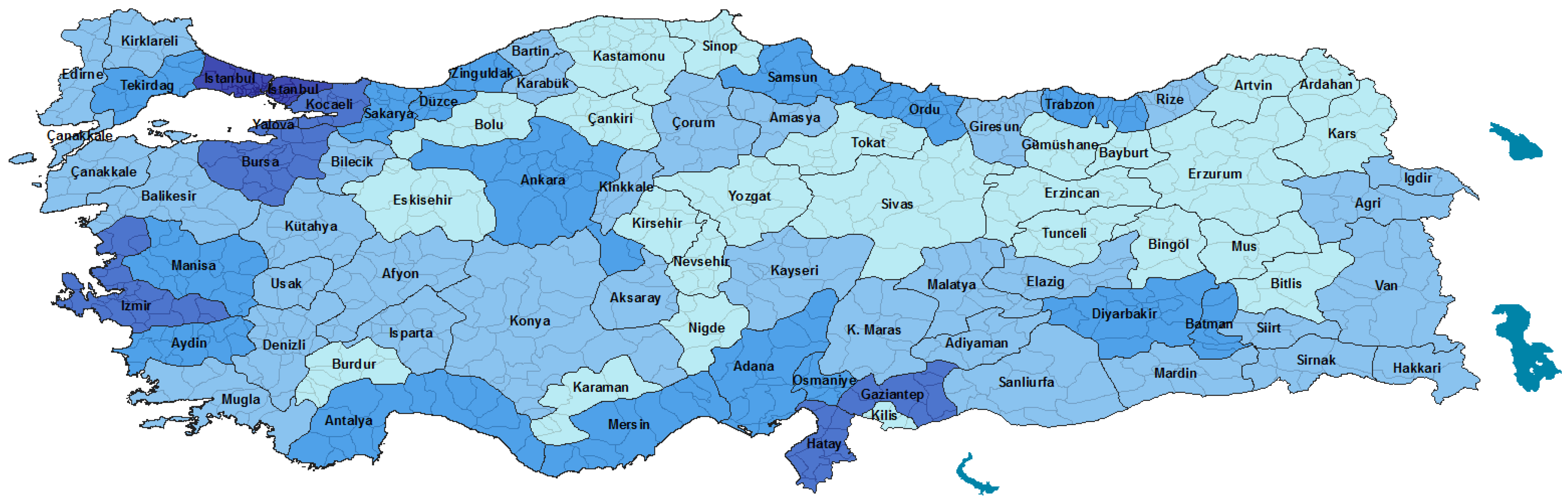
In the attack scenario being addressed, the land force weapon capabilities and land force soldiers of each bordering country are assumed to be distributed evenly across the Turkish cities located on that country’s border with Turkey. For example (see the map in Figure 1), Edirne is located on the border with Greece. Therefore, all Greece’s land force capabilities (soldiers and weapons) are assumed to attack from Edirne. As another example, Ağrı, Iğdır, and Van are located on the border with Armenia. Therefore, Armenia’s land force capabilities are divided into three equal portions, each portion is assumed to attack from one city, and all attacks take place at the same time.

4.2.2. Nodes and Weapon Types

The set of candidate locations N is considered to be the set of Turkish cities to which quantities of weapons are allocated; throughout this paper, these cities are referred to as supply cities. The set of demand points M is considered to be the set of bordering Turkish cities to which weapons must be supplied to defend the country against attacks; throughout this document, these cities are referred to as bordering cities. The set of product types P is considered to be the set of weapon types (in Table 1).

4.2.3. Supply

${\mathrm{s}}_{\mathrm{k}}$, the available stock of a weapon type k($\mathrm{k}\in \mathrm{P}$), is assumed to be the total quantity that Turkey owns in its stock of that weapon type.

Table 2. Turkey’s capacity of weapon types. For more information on data sources, please refer to Section 4.1 (Data Sources).

Weapon Type	Stock
Turkey: AFV: AIFV	650
Turkey: AFV: APC	3643
Turkey: AFV: ARV	0
Turkey: AT: GUNS	0
Turkey: AFV: MBT	2504
Turkey: ARTY: MOR	5813
Turkey: ARTY: MRL	146
Turkey: AT: MSL	1363
Turkey: AT: MSL SP	365
Turkey: AT: RCL	3869
Turkey: AFV: RECCE	320
Turkey: ARTY: SP	1133
Turkey: ARTY: TOWED	760
Turkey: Land Forces	402,000

shows Turkey’s capacity of each of the weapon types considered in this study. In Table 2, the stock of each weapon type is the total number of units that Turkey possesses.

4.2.4. Demands

A demand point j’s ($\mathrm{j}\in \mathrm{M}$) demand of a product type k($\mathrm{k}\in \mathrm{P}$), ${\mathrm{d}}_{\mathrm{jk}}$, is considered to be the total amount of a particular weapon type required to defend the country against one or more attacks; in other words, ${\mathrm{d}}_{\mathrm{jk}}$ is the bordering city j’s ($\mathrm{j}\in \mathrm{M}$) total demand of a weapon type k($\mathrm{k}\in \mathrm{P}$) that is required to respond to one or more attacks coming to the bordering city.

Table 3. The number of units demanded of each weapon type at each demand point.

	AĞRI	ARDAHAN	ARTVİN	EDİRNE	GAZİANTEP	HAKKARİ	HATAY	IĞDIR	KARS	KİLİS	KIRKLARELİ	MARDİN	ŞANLIURFA	ŞIRNAK	VAN	TOTAL
AIFV	32	24	24	478	408	324	408	236	57	408	80	408	408	529	203	4027
APC	43	63	63	2614	250	868	250	257	106	250	64	250	250	905	214	6447
ARV	0	0	0	0	0	108	0	0	0	0	0	0	0	107	0	215
GUNS	0	15	15	63	0	0	0	0	20	0	63	0	0	0	0	176
MBT	36	41	41	1394	990	824	990	591	78	990	40	990	990	990	554	9539
MOR	4	21	21	2427	68	2141	68	1671	26	68	108	68	68	544	1666	8969
MRL	17	12	12	159	83	495	83	509	30	83	12	83	83	84	492	2237
MSL	0	10	0	0	730	0	365	0	0	365	0	365	365	365	0	2565
MSL SP	7	0	0	612	68	0	68	7	8	68	12	68	68	69	0	1055
RCL	0	0	0	4508	0	66	0	67	0	0	0	0	0	0	66	4707
RECCE	0	1	1	239	588	48	0	12	2	0	10	0	0	36	11	948
SP	12	22	22	611	83	121	83	110	36	83	24	83	83	108	97	1578
TOWED	44	23	23	565	338	706	338	720	67	338	12	338	338	369	676	4895
Force	13,950	5916	5916	101,650	36,666	143,666	36,666	130,616	19,867	36,666	8150	36,666	36,666	63,667	116,667	793,395

shows the demand for each weapon type at each demand point in this case study.

4.2.5. Risks

${\mathrm{r}}_{\mathrm{ij}}$, which is considered to be the risk of allocating a unit of the supply of demand of a bordering city $\mathrm{j}\in \mathrm{M}$ to city $\mathrm{i}\in \mathrm{N}$, is calculated in terms of the distance between city i and bordering city j. It is assumed that the further city i is from bordering city j, the riskier city j becomes for supplying bordering city j’s demand for any weapon type. The lowest allocation risk is 1, which is assumed to be the shortest distance ${\mathrm{e}}_{\mathrm{ij}}$ between bordering city j and all cities $\mathrm{i}\in \mathrm{N}$. Thus, city i’s risk is calculated as multiples of the shortest distance between bordering city j and all cities $\mathrm{i}\in \mathrm{N}$. All risk values are rounded up to remove fractions.

For example, the distance between ADANA and bordering city AĞRI is 966; the shortest distance to AĞRI is 184; therefore, the risk of allocating one unit of AĞRI’s demand of any weapon type to be supplied from ADANA is:

$$966÷184\simeq 5.25=6.$$

4.2.6. Setup Costs

${\mathrm{u}}_{\mathrm{ik}}$, which is the setup cost of allocating one unit of weapon type $\mathrm{k}\in \mathrm{P}$ to be supplied from city $\mathrm{i}\in \mathrm{N}$. The setup cost for a weapon is usually incurred when the weapon is to be deployed in a city. The cost covers matters such as engineering and configuration time, as well as testing. The setup cost of a weapon type in a supply city is assumed to be proportional to the elevation of that city. Thus, the larger a city’s elevation is, the higher the setup cost of a weapon type in that city becomes. In this study, only artillery weapons are considered to have setup costs. This is because these weapons require adjustment and configuration when deployed, while other weapon types (such as rifles) do not require such measures. The setup cost of a weapon type is calculated using a base value multiplied by the elevation of the supply city. The base values given for artillery weapons are as follows: Mortar is given 0.5, Towed Artillery is given 1, Multiple Rocket Launcher is given 1.5, and Self-Propelled Artillery is given 2.

An example of calculating setup costs is as follows: the base value for a Multiple Rocket Launcher is 1.5; the elevation of supply cities AKSARAY and ANTALYA is 900 and 43, respectively; thus, the setup costs of a Multiple Rocket Launcher in AKSARAY and ANTALYA becomes

$$1.5\times 900=1350$$

and

$$1.5\times 43=64.5$$

Again, values are rounded up to remove fractions. Thus, the setup costs from the example becomes 1350 and 65 for AKSARAY and ANTALYA, respectively.

4.2.7. Supply City Capacities

${\mathrm{p}}_{\mathrm{ik}}$ is the maximum quantity of units of weapon type $\mathrm{k}\in \mathrm{P}$ allowed to be allocated to supply city $\mathrm{i}\in \mathrm{N}$. This value is assumed to be proportional to city population. The larger a city’s population is, the larger that city’s capacity becomes. The capacities of a weapon type for all supply cities are calculated by distributing the total demand ${\sum }_{\mathrm{k}\in \mathrm{P}}{\mathrm{d}}_{\mathrm{jk}}$ of that weapon type to all supply cities based on their population. The fact that bordering cities are not considered as supply cities means their population is consequently not considered in the distribution. Since capacities are calculated based on total demand and each individual city’s population, the total capacity available for allocation would be smaller than the total demand, and would thus cause infeasibility. To overcome this issue, the total population of bordering cities is divided and added to the population of supply cities.

The following example illustrates how capacities are calculated: In this study, the total demand for Main Battle Tanks (MBT), Self-Propelled Artillery (SP), and Towed Artillery (TOWED) are 9539, 1578, and 4895, respectively; the population of supply cities ANKARA, BURSA, and BATMAN, represented as a percentage of Turkey’s population, are 6.7%, 3.6%, and 0.7%, respectively; the total population of bordering cities, represented as a percentage of Turkey’s population, is 12.9%; the total number of candidate supply cities is 66; thus, the capacity of MBTs in ANKARA is calculated as follows:

$$\left(6.7\%+\left(12.9\%÷66\right)\right)\times 9539=657.76\simeq 658$$

The remaining capacities of MBT, SP, and TOWED in supply cities ANKARA, BURSA, and BATMAN are shown in

Table 4. Capacities of cities of weapon types MBT, SP, and TOWED.

	Ankara	Bursa	Batman
MBT	658	366	88
SP	109	61	15
TOWED	338	188	45

.

5. Solution Method

The problem was solved using Microsoft Excel and OpenSolver. Excel was used for defining and organizing the input data and OpenSolver (using the CBC Solver) was used to solve the problem and generate the solution. The XLSX spreadsheet that was created to solve this problem could be used to determine the locations and weapon quantity allocations for other scenarios. The problem was defined and organized in Excel, using 18 tables. The solution values generated by OpenSolver (allocations of quantities of weapon types to supply cities) were also stored in predefined cells in an Excel table.

6. Results and Discussion

The case study was solved in approx. 14 min and the optimal total transportation and setup cost was 755,210,884.00.

Table 5. Problem description, solution infrastructure, and results.

Problem Description and Solution Results
Solution Time	~14 min
# Decision Variables	27,720 variables
# Bordering Cities	15
# Supply Cities	66
Total Cost	755,210,884.00
Solution Infrastructure
Operating System	Windows 7 SP1
RAM	3 GB
CPU	Intel Core 2 Duo
Solver	CBC Solver

shows the environment on which the problem was solved, as well as the solution results. The results of this study can be used to establish facilities for storing weapons all over the country to guarantee that any attack is handled with the minimum cost and risk. In this case, minimum transportation cost also means minimum time, because the transportation cost is calculated in terms of the distance traveled by each unit of a weapon type. The weapon allocations generated in this work considered only one scenario and were based on certain assumptions. More suitable weapon allocations can be achieved by conducting the study on different scenarios and changing the assumptions to accommodate those scenarios. One way of obtaining more suitable weapon allocations is to conduct the study on various attack scenarios, and then analyze the resulting location data from all scenario studies in order to determine locations that suit all attack scenarios.

6.1. Solving Different Attack Scenarios

As mentioned earlier, this case study considers the scenario where Turkey is being attacked by all neighboring countries, and these countries are using their entire land force capabilities. The Excel spreadsheet used to solve the model for this case study can be used to address other scenarios, such as the scenario in which each neighboring country is attacking from a single bordering city, or the scenario in which a neighboring country is using only a portion of its land force military capability. In these scenarios, the spreadsheet can be copied, attack and response table entries deleted, and new ones created to define the new scenario. If the spreadsheet is to be used for scenarios where the weapon types, bordering cities (or demand points), or supply cities are increased or decreased—such as the scenario in which allocation is performed to only a portion of supply cities—then the spreadsheet will require some changes. The required changes need to be made to the rows and columns of these tables: Distances, Risks, Setup Costs, Capacities, Weapon Allocations, and Supply Allocations.

6.2. Limitations and Potential Improvements

There is one known limitation to this work, which is the fact that the study focused only on land force weapons and attacks and ignored other types of military forces and attacks, such as the navy and the air force. The model can be improved in future works to consider this limitation in planning weapon allocations.

This work determines weapon allocations to minimize cost and risk. However, there is no limit on where weapons can be allocated. It might be desirable to limit the locations to which certain weapon types can be allocated. Furthermore, it might also be desirable to limit the number of facilities opened in some way. One way of limiting the number of facilities would be to have the number of weapons allocated to a supply city exceed a predefined threshold for a facility to be opened in that city; otherwise, the allocated quantity of weapons can be reallocated to the nearest opened facility. Another way of limiting the number of facilities would be to limit the number of facilities for each weapon type; or to open a facility in a supply city when there are at least three or more weapon types.

It is also possible to divide the country into regions (two or three) and conduct the study separately for each of the regions.

6.3. Military Perspective Insights

Up until now, the problem is interpreted as a special location-allocation problem, which is faced frequently in the literature. In this section of the paper, the methodology and findings are summarized in a military perspective and the validity of the approach is discussed. In real life, all armies are trained against different attack scenarios. Normally, these drills are conducted, but no written literature can be found during the reviews because of information security issues. However, since it has been a rather long time since 1970, an incoming attack scenario of NATO can be found in this working group report [33]. Upon examination of the document, it can be seen that the assumptions of this study are valid in real life. Armies are trained against similar scenarios in case of incoming attacks. However, this document’s assumptions are not supported by such mathematical models or computations. Thus, the contribution of this study is a mathematical model that is proposed to serve as a decision support tool for real life decisions. Upon examination of the findings, it is seen that the backup is obtained mostly from the closest three cities, which shows the validity of the model. In real life, however, the backup decisions are made regardless of transportation costs, setup costs, or risk evaluations. However, since national security depends highly on economics, these costs can change the march of events. Additionally, the risks of backup weapon shipments are not calculated mathematically by decision makers, but rather they are calculated intuitively. Thus, the results of this experimental study can serve as a real life decision support tool for military officers, since it is valid and effective.

7. Conclusions

Homeland defense is an important matter regardless of the location of the country. Countries need to pay special attention to their defense mechanisms and ensure that they are ready to respond to threats. This work demonstrated how facility location problems can be utilized for military decision making. With this work, we contributed to sustaining Turkey’s homeland defense decision making by introducing a mathematical model for determining the optimal locations for storing quantities of various weapon types to minimize the total transportation and setup costs, as well as the risks associated with weapon locations. The model is tested on a case study in which the scenario of Turkey being attacked by the entire land force of all countries on its border is examined. The model is solved to determine the optimal locations for storing weapons in order to defend the country from such an attack with minimal cost and risk. Since the developed model determined the optimum results for this study, it can be used for critical decision making, and the mathematical models can be used more frequently for military deployment. In the future, the model can be expanded to cover all of the forces of the country, because only the land forces were taken into account in this study. In this case, the problem will be much trickier and meta-heuristics can be developed to make a decision support in short computational times. In the attack scenarios of this paper, the attacking unit numbers are not uncertain, thus this issue can be taken into account in the future. Finally, alternative “what if” scenarios can be proposed to handle the attacks economically.

References

- Weber, A. Theory of the Location of Industries; U.S. Department of Defense, Homeland Defense, Joint Publications 3-27: Washington, DC, USA, 2007.
- Kariv, O.; Hakimi, S.L. An algorithmic approach to network location problems. I: The p-centers. SIAM J. Appl. Math. 1979, 37, 513–538. [Google Scholar] [CrossRef]
- Kariv, O.; Hakimi, S.L. An algorithmic approach to network location problems. Ii: The p-medians. SIAM J. Appl. Math. 1979, 37, 539–560. [Google Scholar] [CrossRef]
- Melkote, S.; Daskin, M.S. Capacitated facility location/network design problems. Eur. J. Oper. Res. 2001, 129, 481–495. [Google Scholar] [CrossRef]
- Tran, T.H.; Scaparra, M.P.; O’Hanley, J.R. A hypergraph multi-exchange heuristic for the single-source capacitated facility location problem. Eur. J. Oper. Res. 2017, 263, 173–187. [Google Scholar] [CrossRef]
- Revelle, C.S.; Eiselt, H.A.; Daskin, M.S. A bibliography for some fundamental problem categories in discrete location science. Eur. J. Oper. Res. 2008, 184, 817–848. [Google Scholar] [CrossRef]
- Sridharan, R. The capacitated plant location problem. Eur. J. Oper. Res. 1995, 2, 203–213. [Google Scholar] [CrossRef]
- Gendron, B.; Khuong, P.V.; Semet, F. Comparison of formulations for the two-level uncapacitated facility location problem with single assignment constraints. Comput. Oper. Res. 2017, 86, 86–93. [Google Scholar] [CrossRef]
- Ravi, R.; Sinha, A. Multicommodity facility location. In Proceedings of the SODA ’04 Fifteenth Annual ACM-SIAM Symposium on Discrete Algorithms, New Orleans, LA, USA, 11–13 January 2004. [Google Scholar]
- Eiselt, H.A.; Sandblom, C.L. Decision Analysis, Location Models, and Scheduling Problems; Springer Science & Business Media: Berlin, Germany, 2013. [Google Scholar]
- Schilling, D.A.; Jayaraman, V.; Barkhi, R. A review of covering problem in facility location. Locat. Sci. 1993, 1, 25–55. [Google Scholar]
- Toregas, C.; Swain, R.; ReVelle, C.; Bergman, L. The location of emergency service facilities. Oper. Res. 1971, 19, 1363–1373. [Google Scholar] [CrossRef]
- Beasley, J.E.; Chu, P.C. A genetic algorithm for the set covering problem. Eur. J. Oper. Res. 1996, 2, 392–404. [Google Scholar] [CrossRef]
- Eaton, D.J.; Daskin, M.S.; Simmons, D.; Bulloch, B.; Jansma, G. Determining emergency medical service vehicle deployment in austin, texas. Interfaces 1985, 1, 96–108. [Google Scholar] [CrossRef]
- Dyer, M.E.; Frieze, A.M. A simple heuristic for the p-centre problem. Oper. Res. Lett. 1985, 6, 285–288. [Google Scholar] [CrossRef]
- Davidović, T.; Ramljak, D.; Šelmić, M.; Teodorović, D. Bee colony optimization for the p-center problem. Comput. Oper. Res. 2011, 38, 1367–1376. [Google Scholar] [CrossRef]
- Irawan, C.A.; Salhi, S.; Drezner, Z. Hybrid meta-heuristics with VNS and exact methods: Application to large unconditional and conditional vertex p-centre problems. J. Heurist. 2016, 22, 507–537. [Google Scholar] [CrossRef] [Green Version]
- Callaghan, B.; Salhi, S.; Nagy, G. Speeding up the optimal method of drezner for the p-centre problem in the plane. Eur. J. Oper. Res. 2017, 257, 722–734. [Google Scholar] [CrossRef] [Green Version]
- Laporte, G.; Nickel, S.; da Gama, F.S. Location Science; Springer: Berlin, Germany, 2015. [Google Scholar]
- Goldman, A.J. Optimal center location in simple networks. Transp. Sci. 1971, 5, 212–221. [Google Scholar] [CrossRef]
- Ndiaye, F.; Ndiaye, B.M.; Ly, I. Application of the p-median problem in school allocation. Am. J. Oper. Res. 2012, 2, 253–259. [Google Scholar] [CrossRef]
- Dzator, M.; Dzator, J. An effective heuristic for the p-median problem with application to ambulance location. Opsearch 2013, 50, 60–74. [Google Scholar] [CrossRef]
- Cooper, L. Location-allocation problems. Oper. Res. 1963, 11, 331–343. [Google Scholar] [CrossRef]
- Aboolian, R.; Sun, Y.; Koehler, G.J. A location–allocation problem for a web services provider in a competitive market. Eur. J. Oper. Res. 2009, 194, 64–77. [Google Scholar] [CrossRef]
- Zhang, W.; Cao, K.; Liu, S.; Huang, B. A multi-objective optimization approach for health-care facility location-allocation problems in highly developed cities such as Hong Kong. Comput. Environ. Urban Syst. 2016, 59, 220–230. [Google Scholar] [CrossRef]
- Zarrinpoor, N.; Fallahnezhad, M.S.; Pishvaee, M. Design of a reliable hierarchical location-allocation model under disruptions for health service networks: A two-stage robust approach. Comput. Ind. Eng. 2017, 109, 130–150. [Google Scholar] [CrossRef]
- Jaiswal, N.K. Military Operations Research: Quantitative Decision Making; International Series in Operations Research & Management Science; Springer: Berlin, Germany, 1997. [Google Scholar]
- Ahuja, R.K.; Kumar, A.; Jha, K.C.; Orlin, J.B. Exact and heuristic algorithms for the weapon-target assignment problem. Oper. Res. 2007, 55, 1136–1146. [Google Scholar] [CrossRef]
- Leboucher, C.; Shin, H.S.; Le Ménec, S.; Tsourdos, A.; Kotenkoff, A.; Siarry, P.; Chelouah, R. Novel evolutionary game based multi-objective optimisation for dynamic weapon target assignment. IFAC Proc. Vol. 2014, 47, 3936–3941. [Google Scholar] [CrossRef]
- Kalyanam, K.; Rathinam, S.; Casbeer, D.; Pachter, M. Optimal threshold policy for sequential weapon target assignment. IFAC-PapersOnLine 2016, 49, 7–10. [Google Scholar] [CrossRef]
- Yan, Y.; Zha, Y.; Qin, L.; Xu, K. A research on weapon-target assignment based on combat capabilities. In Proceedings of the 2016 IEEE International Conference Mechatronics and Automation (ICMA), Harbin, China, 7–10 August 2016; pp. 2403–2407. [Google Scholar]
- Montoya, A.; Vélez–Gallego, M.C.; Villegas, J.G. Multi-product capacitated facility location problem with general production and building costs. NETNOMICS Econ. Res. Electron. Netw. 2016, 17, 47–70. [Google Scholar] [CrossRef]
- Interagency Working Group 5 For National Security Memorandum 84, The Warsaw Pact Threat to NATO, 1970. Available online: https://www.cia.gov/library/readingroom/docs/1970-05-01.pdf (accessed on 27 April 2018).
Figure 1.
Map of Turkey; for higher resolution, please visit: https://commons.wikimedia.org/wiki/File:Turkey,_administrative_divisions_-_de.svg.