Some New Contributions on the Marshall–Olkin Length Biased Lomax Distribution: Theory, Modelling and Data Analysis

Abstract

The Lomax distribution is arguably one of the most useful lifetime distributions, explaining the developments of its extensions or generalizations through various schemes. The Marshall–Olkin length-biased Lomax distribution is one of these extensions. The associated model has been used in the frameworks of data fitting and reliability tests with success. However, the theory behind this distribution is non-existent and the results obtained on the fit of data were sufficiently encouraging to warrant further exploration, with broader comparisons with existing models. This study contributes in these directions. Our theoretical contributions on the the Marshall–Olkin length-biased Lomax distribution include an original compounding property, various stochastic ordering results, equivalences of the main functions at the boundaries, a new quantile analysis, the expressions of the incomplete moments under the form of a series expansion and the determination of the stress–strength parameter in a particular case. Subsequently, we contribute to the applicability of the Marshall–Olkin length-biased Lomax model. When combined with the maximum likelihood approach, the model is very effective. We confirm this claim through a complete simulation study. Then, four selected real life data sets were analyzed to illustrate the importance and flexibility of the model. Especially, based on well-established standard statistical criteria, we show that it outperforms six strong competitors, including some extended Lomax models, when applied to these data sets. To our knowledge, such comprehensive applied work has never been carried out for this model.

1. Introduction

The Lomax distribution introduced by [1] can be described as a simple two-parameter lifetime distribution with a varying polynomial decay. By denoting the shape parameter as $\alpha >0$ and the scale parameter as $\beta >0$, it is specified by the following probability density function (pdf):

$$f_L(x;\alpha ,\beta )=\frac{\alpha }{\beta }{\left(1+\frac{x}{\beta }\right)}^{-(\alpha +1)},x\ge 0,$$

(1)

and $f_L(x;\alpha ,\beta )=0$ for $x<0$. Basically, the Lomax distribution corresponds to the famous Pareto distribution that has been shifted to the left until its support starts at 0 (see [2], p. 573). It has been widely used for the modeling of various measures in reliability and life testing from heavy tailed data. The literature on the Lomax distribution and its applications is vast, including [3,4,5,6,7,8,9], to name of few.

In order to make the statistical possibilities of the Lomax distribution more flexible and attractive, several multiple-parameter modifications and generalizations have been proposed. Among them, we cite the Marshall–Olkin Lomax distribution by [10], transmuted Lomax distribution by [11], MacDonald Lomax distribution by [12], Poisson Lomax distribution by [13], exponentiated Lomax distribution by [14], exponential Lomax distribution by [15], gamma Lomax distribution by [16], Weibull Lomax distribution by [17], weighted Lomax distribution by [18], power Lomax distribution by [19], length-biased Lomax by [20], half-logistic Lomax distribution by [21], Marshall–Olkin power Lomax by [22] and Marshall–Olkin length-biased Lomax by [23], among others.

In particular, based on the concept of length-biased distribution pioneered by [20,24] introduced the length-biased Lomax (LBLO) distribution with the following pdf:

$$f_{LBLO}(x;\alpha ,\beta )=\frac{1}{{\mu }_L}x{f}_L(x;\alpha ,\beta ),x\in \mathbb{R},$$

where ${\mu }_L$ denotes the mean of the Lomax distribution. That is, by taking into account that ${\mu }_L=\beta /(\alpha -1)$ for $\alpha >1$, the pdf above can be expressed as

$$f_{LBLO}(x;\alpha ,\beta )=\frac{\alpha (\alpha -1)}{{\beta }^2}x{\left(1+\frac{x}{\beta }\right)}^{-(\alpha +1)},x\ge 0,$$

(2)

for $\alpha >1$ and $\beta >0$, and $f_{LBLO}(x;\alpha ,\beta )=0$ for $x<0$. One can remark that $f_{LBLO}(0;\alpha ,\beta )=0$ against $f_L(0;\alpha ,\beta )=\alpha /\beta$. Thus the parameters $\alpha$ and $\beta$ only governed the shapes of the pdf independently of the values of the initial value, contrary to the former Lomax distribution, while keeping a similar level of flexibility. In this sense, for some applied problems, the LBLO model is an interesting alternative to the Lomax model, with the same number of parameters. Further detail can be found in [20].

Recently, [23] proposed a new extension of the LBLO distribution called Marshall–Olkin length-biased Lomax (MOLBL) distribution. It consists in modifying the LBLO distribution via the Marshall–Olkin scheme pioneered by [25]. The aim is to add more flexibility to the LBLO distribution through ratio-type definitions of the main functions depending on a tuning parameter. Precisely, the corresponding pdf with the shape parameters $\alpha >0$ and $\gamma >0$, and scale parameter $\beta >0$ is

$$\begin{array}{c}\hfill f_{MOLBL}(x;\alpha ,\beta ,\gamma )=\frac{\alpha (\alpha -1)\gamma }{{\beta }^2}\frac{x{(1+x/\beta )}^{-(\alpha +1)}}{{\left[1-(1-\gamma ){(1+x/\beta )}^{-\alpha }(1+\alpha x/\beta )\right]}^2},x\ge 0,\end{array}$$

(3)

and $f_{MOLBL}(x;\alpha ,\beta ,\gamma )$ for $x<0$. Thus, the parameter $\gamma$ modulates the denominator function; the LBLO distribution being recovered by taking $\gamma =1$. In [23], the parameters of the MOLBL model are estimated by the maximum likelihood estimation method, without convergence evidence. The remission data set by [26] is analyzed, and it is proved that the MOLBL model has a better fit to the former LBLO model by considering the Akaike information criterion (AIC) and Bayesian information criterion (BIC), only. In addition, a reliability test plan is developed to accept or reject a submitted lot of products for inspection whose lifetime is directed to be a MOLBL distribution.

In this study, we complete the study of [23] on several important aspects, making significant theoretical and practical contributions to the MOLBL distribution. For the theoretical findings, (i) we prove that the MOLBL distribution can be derived by a simple compounding argument, (ii) new stochastic ordering properties are established, (iii) asymptotic equivalences are described for the first time with discussion on the role played by the parameters in this regard, (iv) a quantile analysis is performed with a special focus on the case $\alpha =2$, (v) the incomplete moments are expressed, as well as the ordinary moments, and (vi) the stress–strength parameter is determined for a special configuration on the parameters. For the practical contributions, (a) a complete simulation study guaranties the numerical convergence of the maximum likelihood estimates, (b) four different data sets are considered, and (c), for these data sets, six competitors are used, including some extended Lomax distributions. We show that the MOLBL model is the best based on the following benchmarks: AIC as well as its consistent version (CAIC), BIC, Hannan–Quinn information criterion (HQIC), Anderson–Darling ($A^{*}$), Cramer–von Mises ($W^{*}$), Kolmogorov–Smirnov (KS) and the p-value of the corresponding KS statistical test. A graphical analysis of the obtained fits is also provided, showing the high quality of the MOLBL model.

The paper is as follows. Section 2 is devoted to the theoretical contributions on the MOLBL distribution. Section 3 completes the above by offering the practical contributions. Finally, Section 4 contains some concluding remarks.

2. Theoretical Contributions

This section is devoted to new theoretical facts about the MOLBL distribution.

2.1. Main Functions of the MOLBL Distribution

We now recall the main functions of the MOLBL distribution, as sketched in [23]. First, the cumulative distribution function (cdf) of the MOLBL distribution is given as

$$\begin{array}{c}\hfill F_{MOLBL}(x;\alpha ,\beta ,\gamma )=\frac{1-{(1+x/\beta )}^{-\alpha }(1+\alpha x/\beta )}{1-(1-\gamma ){(1+x/\beta )}^{-\alpha }(1+\alpha x/\beta )},x\ge 0,\end{array}$$

(4)

and $F_{MOLBL}(x;\alpha ,\beta ,\gamma )=0$ for $x<0$. The cdf of the LBLO distribution is obtained as a special case; it follows by substituting $\gamma =1$ in Equation (4). Based on Equation (4), the survival function (sf) of the MOLBL distribution can be expressed as

$$\begin{array}{c}\hfill S_{MOLBL}(x;\alpha ,\beta ,\gamma )=\gamma \frac{{(1+x/\beta )}^{-\alpha }(1+\alpha x/\beta )}{1-(1-\gamma ){(1+x/\beta )}^{-\alpha }(1+\alpha x/\beta )},x\ge 0,\end{array}$$

(5)

and $S_{MOLBL}(x;\alpha ,\beta ,\gamma )=1$ for $x<0$. We recall that the pdf of the MOLBL distribution is specified by Equation (3), corresponding to the derivative of $F_{MOLBL}(x;\alpha ,\beta ,\gamma )$ with respect to x. From Equations (3) and (5), we can express the hazard rate function (hrf) of the MOLBL distribution by

$$\begin{array}{c}\hfill h_{MOLBL}(x;\alpha ,\beta ,\gamma )=\frac{\alpha (\alpha -1)}{{\beta }^2}\frac{x}{\left[1-(1-\gamma ){(1+x/\beta )}^{-\alpha }(1+\alpha x/\beta )\right](1+x/\beta )(1+\alpha x/\beta )},x\ge 0,\end{array}$$

(6)

and $h_{MOLBL}(x;\alpha ,\beta ,\gamma )=0$ for $x<0$. The above analytical definitions are fundamental to explore the possibilities of the MOLBL model. They are used intensively in the remainder of the paper.

For the purposes of this study, the MOLBL distribution is denoted as MOLBL$(\alpha ,\beta ,\gamma )$ distribution when the parameters must be communicated.

2.2. Compounding

The following proposition shows that the MOLBL distribution follows from a special compounding distribution involving the classical exponential distribution with parameter $\gamma$.

Proposition 1.

Let X and Y be continuous random variables such that

• the conditional cdf of$X\mid \{Y=y\}$is given as

  $$\begin{array}{c}\hfill F_o(x;\alpha ,\beta \mid y)=1-exp\left\{-\left[{\left(1+\frac{x}{\beta }\right)}^{\alpha }{\left(1+\frac{\alpha x}{\beta }\right)}^{-1}-1\right]y\right\},y\ge 0,\end{array}$$

  (7)

  which is a well-identified cdf specified later,
• Y has the exponential distribution with parameter$\gamma >0$, that is with the pdf defined by$f_E(y;\gamma )=\gamma e^{-\gamma y}$for$y\ge 0$and$f_E(y;\gamma )=0$for$y<0$.

Then X has the MOLBL$(\alpha ,\beta ,\gamma )$distribution.

Proof. 

By using the distribution of X conditionally to $\{Y=y\}$, the cdf of X is obtained as

$$\begin{array}{cc}\hfill F_{*}(x;\alpha ,\beta ,\gamma )& ={\int }_0^{+\infty }{F}_o(x;\alpha ,\beta \mid y)f_E(y;\gamma )dy\hfill \\ \hfill & =1-{\int }_0^{+\infty }[1-F_o(x;\alpha ,\beta \mid y)]f_E(y;\gamma )dy\hfill \\ \hfill & =1-{\int }_0^{+\infty }exp\left\{-\left[{\left(1+\frac{x}{\beta }\right)}^{\alpha }{\left(1+\frac{\alpha x}{\beta }\right)}^{-1}-1\right]y\right\}\gamma e^{-\gamma y}dy\hfill \\ \hfill & =1-\gamma {\int }_0^{+\infty }exp\left\{-\left[{\left(1+\frac{x}{\beta }\right)}^{\alpha }{\left(1+\frac{\alpha x}{\beta }\right)}^{-1}-(1-\gamma )\right]y\right\}dy\hfill \\ \hfill & =1-\gamma {\left[{\left(1+\frac{x}{\beta }\right)}^{\alpha }{\left(1+\frac{\alpha x}{\beta }\right)}^{-1}-(1-\gamma )\right]}^{-1}\hfill \\ \hfill & =1-\gamma \frac{{(1+x/\beta )}^{-\alpha }(1+\alpha x/\beta )}{1-(1-\gamma ){(1+x/\beta )}^{-\alpha }(1+\alpha x/\beta )}=1-S_{MOLBL}(x;\alpha ,\beta ,\gamma )\hfill \\ \hfill & =F_{MOLBL}(x;\alpha ,\beta ,\gamma ).\hfill \end{array}$$

This entails the desired result. ☐

As announced, the conditional cdf of $X\mid \{Y=y\}$ expressed in Equation (7) is well identified; it corresponds to the cdf of the Weibull-G family of distributions by [27] defined with the parameters $\tilde{\alpha }=y$ and $\tilde{\beta }=1$, and with the LBLO distribution as parental distribution. However, to our knowledge, it has not received a special attention, and can be the object of a future study.

2.3. Stochastic Ordering

The notion of first-order stochastic dominance is the most basic stochastic ordering concept. It consists in giving a mathematical setting to compare several distributions through their cdfs or, equivalently, their sfs. More precisely, we say that a distribution symbolized by A first-order stochastically dominates (FOSD) a distribution symbolized by B if their respective cdfs, say $F_A\left(x\right)$ and $F_B\left(x\right)$, satisfy the following inequality: $F_A\left(x\right)\le F_B\left(x\right)$, for all $x\in \mathbb{R}$. This concept finds numerous applications in actuarial sciences, econometrics, reliability and biometrics. One may refer to [28,29].

The next result shows several first order stochastic order dominance results for the MOLBL distributions based on all its parameters.

Proposition 2.

The following results hold.

(i)

For${\alpha }_1\le {\alpha }_2$, the MOLBL$({\alpha }_1,\beta ,\gamma )$distribution FOSD the MOLBL$({\alpha }_2,\beta ,\gamma )$distribution.

(ii)

For${\beta }_1\le {\beta }_2$, the MOLBL$(\alpha ,{\beta }_2,\gamma )$distribution FOSD the MOLBL$(\alpha ,{\beta }_1,\gamma )$distribution.

(iii)

For${\gamma }_1\le {\gamma }_2$, the MOLBL$(\alpha ,\beta ,{\gamma }_2)$distribution FOSD the MOLBL$(\alpha ,\beta ,{\gamma }_1)$distribution.

Proof. 

(i)

It is enough to study the monotonicity of $F_{MOLBL}(x;\alpha ,\beta ,\gamma )$ in Equation (4) with respect to $\alpha$. After derivatives and standard manipulations, for $x\ge 0$, we get

$$\begin{array}{c}\hfill \frac{\partial }{\partial \alpha }{F}_{MOLBL}(x;\alpha ,\beta ,\gamma )=\beta \gamma \frac{{(1+x/\beta )}^{\alpha }\left[(\alpha x+\beta )log(1+x/\beta )-x\right]}{{\left[\beta {(1+x/\beta )}^{\alpha }-(1-\gamma )(\alpha x+\beta )\right]}^2}.\end{array}$$

Now, the following logarithmic inequality is well-known: $log(1+y)\ge y/(1+y)$ for $y>-1$. By applying it with $y=x/\beta >0$ and using $\alpha >1$, we have

$$(\alpha x+\beta )log(1+x/\beta )-x\ge (\alpha x+\beta )\frac{x/\beta }{1+x/\beta }-x\ge (x+\beta )\frac{x/\beta }{1+x/\beta }-x=0.$$

Therefore, $\partial F_{MOLBL}(x;\alpha ,\beta ,\gamma )/\partial \alpha \ge 0$, implying that $F_{MOLBL}(x;\alpha ,\beta ,\gamma )$ is an increasing function with respect to $\alpha$; For ${\alpha }_1\le {\alpha }_2$, the MOLBL$({\alpha }_1,\beta ,\gamma )$ distribution FOSD the MOLBL$({\alpha }_2,\beta ,\gamma )$ distribution.

(ii)

Now, let us study the monotonicity of $F_{MOLBL}(x;\alpha ,\beta ,\gamma )$ with respect to $\beta$. After some developments, for $x\ge 0$, we get

$$\begin{array}{c}\hfill \frac{\partial }{\partial \beta }{F}_{MOLBL}(x;\alpha ,\beta ,\gamma )=-(\alpha -1)\alpha \gamma \frac{x^2{(1+x/\beta )}^{\alpha }}{(\beta +x){\left[\beta {(1+x/\beta )}^{\alpha }-(1-\gamma )(\alpha x+\beta )\right]}^2}.\end{array}$$

Since $\alpha >1$, this partial derivative is clearly negative. Hence, $F_{MOLBL}(x;\alpha ,\beta ,\gamma )$ is a decreasing function with respect to $\beta$; For ${\beta }_1\le {\beta }_2$, the MOLBL$(\alpha ,{\beta }_2,\gamma )$ distribution FOSD the MOLBL$(\alpha ,{\beta }_1,\gamma )$ distribution.

(iii)

The monotonicity of $F_{MOLBL}(x;\alpha ,\beta ,\gamma )$ with respect to $\gamma$ is now investigated. After some algebraic manipulations, for $x\ge 0$, we have

$$\begin{array}{c}\hfill \frac{\partial }{\partial \gamma }{F}_{MOLBL}(x;\alpha ,\beta ,\gamma )=\frac{(\alpha x+\beta )\left[\alpha x+\beta -\beta {(1+x/\beta )}^{\alpha }\right]}{{\left[\beta {(1+x/\beta )}^{\alpha }-(1-\gamma )(\alpha x+\beta )\right]}^2}.\end{array}$$

Since $\alpha >1$, the Bernoulli inequality implies that

$$\beta {\left(1+\frac{x}{\beta }\right)}^{\alpha }\ge \beta \left(1+\frac{\alpha }{\beta }x\right)=\alpha x+\beta .$$

Therefore, $\partial F_{MOLBL}(x;\alpha ,\beta ,\gamma )/\partial \gamma \le 0$, implying that $F_{MOLBL}(x;\alpha ,\beta ,\gamma )$ is a decreasing function with respect to $\gamma$; for ${\gamma }_1\le {\gamma }_2$, the MOLBL$(\alpha ,\beta ,{\gamma }_2)$ distribution FOSD the MOLBL$(\alpha ,\beta ,{\gamma }_1)$ distribution.

The proof of Proposition 2 ends. ☐

The next result is about a hazard rate ordering satisfied by the MOLBL distribution. We say that a distribution symbolized by A dominates a distribution symbolized by B in the hazard rate ordering if their respective hrfs, say $h_A\left(x\right)$ and $h_B\left(x\right)$, satisfy the following inequality: $h_A\left(x\right)\le h_B\left(x\right)$, for all $x\in \mathbb{R}$. This kind of stochastic ordering is a useful concept in reliability and order statistics (see [30]).

Proposition 3.

For${\gamma }_1\le {\gamma }_2$, the MOLBL$(\alpha ,\beta ,{\gamma }_2)$distribution dominates the MOLBL$(\alpha ,\beta ,{\gamma }_1)$distribution in the hazard rate ordering.

Proof. 

On the basis of Equation (6), after differentiation and standard operations, we obtain

$$\begin{array}{c}\hfill \frac{\partial }{\partial \gamma }{h}_{MOLBL}(x;\alpha ,\beta ,\gamma )=-{\beta }^2\frac{x{(1+x/\beta )}^{\alpha -1}}{{\left[\beta {(1+x/\beta )}^{\alpha }-(1-\gamma )(\alpha x+\beta )\right]}^2},\end{array}$$

which is clearly negative. Therefore, $h_{MOLBL}(x;\alpha ,\beta ,\gamma )$ is decreasing with respect to $\gamma$, implying that, for ${\gamma }_1\le {\gamma }_2$, $h_{MOLBL}(x;\alpha ,\beta ,{\gamma }_2)\le h_{MOLBL}(x;\alpha ,\beta ,{\gamma }_1)$. This ends the proof of Proposition 3. ☐

Note that, by the relation between the first-stochastic order dominance and hazard rate ordering, Proposition 3 implies Proposition 2 (iii).

2.4. Equivalences

The asymptotic behaviors of the main functions of the MOLBL distribution are useful to understand the role of the parameters played in the limit bounds and also, to prove the existence of important probabilistic quantities such as the moments. When x tends to 0, since the following equivalence at the order two holds:

$${\left(1+\frac{x}{\beta }\right)}^{-\alpha }\sim 1-\alpha \frac{x}{\beta }+\frac{\alpha (\alpha +1)}{2}\frac{x^2}{{\beta }^2},$$

we have

$$F_{MOLBL}(x;\alpha ,\beta ,\gamma )\sim \frac{\alpha (\alpha -1)}{2\gamma {\beta }^2}{x}^2,f_{MOLBL}(x;\alpha ,\beta ,\gamma )\sim h_{MOLBL}(x;\alpha ,\beta ,\gamma )\sim \frac{\alpha (\alpha -1)}{\gamma {\beta }^2}x.$$

The last result implies that both $f_{MOLBL}(x;\alpha ,\beta ,\gamma )$ and $h_{MOLBL}(x;\alpha ,\beta ,\gamma )$ tend to 0 with a polynomial rate of degree 1. When x tends to $+\infty$, the following equivalences hold:

$$F_{MOLBL}(x;\alpha ,\beta ,\gamma )\sim 1-\alpha {\left(\frac{x}{\beta }\right)}^{-\alpha +1},f_{MOLBL}(x;\alpha ,\beta ,\gamma )\sim \frac{\alpha (\alpha -1)}{\beta }{\left(\frac{x}{\beta }\right)}^{-\alpha }$$

and

$$h_{MOLBL}(x;\alpha ,\beta ,\gamma )\sim \frac{\alpha -1}{x}.$$

Therefore, $f_{MOLBL}(x;\alpha ,\beta ,\gamma )$ and $h_{MOLBL}(x;\alpha ,\beta ,\gamma )$ tend to 0 under all circumstances. This convergence is with a polynomial decay with degree $\alpha$ for $f_{MOLBL}(x;\alpha ,\beta ,\gamma )$, and with a polynomial decay with degree 1 for $h_{MOLBL}(x;\alpha ,\beta ,\gamma )$.

As a consequence, by the obtained equivalence: When x tends to $+\infty$, $x^s{f}_{MOLBL}(x;\alpha ,\beta ,\gamma )\sim \alpha (\alpha -1){\beta }^{\alpha -1}{x}^{s-\alpha }$, the Riemann integral criteria ensures that the integral ${\int }_0^{+\infty }{x}^s{f}_{MOLBL}(x;\alpha ,\beta ,\gamma )dx$ exists for $-1<s<\alpha -1$, implying the existence of the $s^{th}$ moments of the MOLBL distribution for any positive integer s satisfying this condition. Also, with a similar argument, we show that, for all $t>0$, ${\int }_0^{+\infty }{e}^{tx}{f}_{MOLBL}(x;\alpha ,\beta ,\gamma )dx=+\infty$, meaning that the MOLBL distribution has a heavy (right) tail.

2.5. Quantile Analysis

Quantile analysis provides precise information on the central and dispersion properties of a distribution. In the setting of the MOLBL distribution, the quantile function, say $Q_{MOLBL}(u;\alpha ,\beta ,\gamma )$, satisfies the following equation: $F_{MOLBL}(Q_{MOLBL}(u;\alpha ,\beta ,\gamma );\alpha ,\beta ,\gamma )=u$ for any $u\in (0,1)$, that is, after a rearrangement,

$${\left(1+\frac{Q_{MOLBL}(u;\alpha ,\beta ,\gamma )}{\beta }\right)}^{-\alpha }\left(1+\frac{\alpha Q_{MOLBL}(u;\alpha ,\beta ,\gamma )}{\beta }\right)=\frac{1-u}{\gamma +(1-\gamma )(1-u)}.$$

In full generality, $Q_{MOLBL}(u;\alpha ,\beta ,\gamma )$ has not a closed-form expression. Only the case $\alpha =2$ is manageable by the analytical approach; In this special case, we have

$$Q_{MOLBL}(u;2,\beta ,\gamma )=\frac{\beta }{1-u}\left(\gamma u+\sqrt{\gamma u[\gamma +(1-\gamma \left)\right(1-u)}]\right).$$

The median is obtained as $M=Q_{MOLBL}(1/2;2,\beta ,\gamma )=\beta (\gamma +\sqrt{\gamma (\gamma +1)})$. Similarly, the first and third quartiles are specified by substituting $u=1/4$ and $u=3/4$ in $Q_{MOLBL}(u;2,\beta ,\gamma )$, respectively. Also, this quantile function can be used for simulated values from the MOLBL distribution.

2.6. Incomplete Moments

The interests of the incomplete moment of a random variable or a distribution are (i) to generalize the notion of ordinary moments, (ii) to be involved in the definitions of important curves, deviation measures and functions, such as the Lorenz curve, mean deviation about the mean and mean residual life function. Discussions and applications on incomplete moments are available in [31,32]. Here, the incomplete moments of the MOLBL distribution are investigated, with discussion on the ordinary moments as well.

First, we need the following general integral result.

Lemma 1.

For any integer $a\ge 0$, and real numbers $b>0$, $c>0$ and $t\ge 0$, let us set

$$\begin{array}{c}\hfill \mathcal{I}(t;a,b,c)={\int }_0^t{x}^a{\left(1+\frac{x}{c}\right)}^{-b}dx.\end{array}$$

(8)

Then, the following sum formula is valid:

$$\begin{array}{c}\hfill \mathcal{I}(t;a,b,c)=c^{a+1}\sum _{j=0}^a\left(\genfrac{}{}{0pt}{}{a}{j}\right){(-1)}^{a-j}\frac{1}{j-b+1}\left[{\left(1+\frac{t}{c}\right)}^{j-b+1}-1\right].\end{array}$$

This equality is true for $t\to +\infty$ provided to $b>1+a$, and we have

$$\begin{array}{c}\hfill \mathcal{I}(+\infty ;a,b,c)=c^{a+1}\sum _{j=0}^a\left(\genfrac{}{}{0pt}{}{a}{j}\right){(-1)}^{a-j+1}\frac{1}{j-b+1}.\end{array}$$

Proof. 

By performing the change of variables $y=1+x/c$, that is, $x=c(y-1)$, we obtain

$$\begin{array}{c}\hfill \mathcal{I}(t;a,b,c)=c^{a+1}{\int }_1^{1+t/c}{(y-1)}^a{y}^{-b}dy.\end{array}$$

Since a is a positive integer, the classical binomial formula holds and we obtain

$$\begin{array}{cc}\hfill \mathcal{I}(t;a,b,c)& =c^{a+1}\sum _{j=0}^a\left(\genfrac{}{}{0pt}{}{a}{j}\right){(-1)}^{a-j}{\int }_1^{1+t/c}{y}^{j-b}dy\hfill \\ \hfill & =c^{a+1}\sum _{j=0}^a\left(\genfrac{}{}{0pt}{}{a}{j}\right){(-1)}^{a-j}\frac{1}{j-b+1}\left[{\left(1+\frac{t}{c}\right)}^{j-b+1}-1\right].\hfill \end{array}$$

For the case $t\to +\infty$, it is enough to notice that, for $b>1+a$, we have $j-b+1<a-b+1<0$, implying that ${(1+t/c)}^{j-b+1}$ tends to 0. The desired result follows. This ends the proof of Lemma 1. ☐

Lemma 1 can be used independently of interest, but will be at the heart for manageable series expression of the incomplete moments.

We are in the position to present the main results of this section, regarding the incomplete moments of the MOLBL distribution. The proposition below proposes a series expansion of any of these incomplete moments in the case $\gamma \in (0,1)$.

Proposition 4.

Let s be an integer and X be a random variable having the MOLBL$(\alpha ,\beta ,\gamma )$ distribution with $\gamma \in (0,1)$. Then, for $t\ge 0$, the $s^{th}$ incomplete moment of X according to t is given as

$$\begin{array}{cc}\hfill {\mu }_s^{\prime }\left(t\right)& =E\left(X^{s}I\left(\{X\le t\}\right)\right)=\sum _{k=0}^{+\infty }\sum _{\ell =0}^k\sum _{j=0}^{s+\ell +1}{\Delta }_{k,\ell ,j;s}\left[{\left(1+\frac{t}{\beta }\right)}^{j-\alpha (k+1)}-1\right],\hfill \end{array}$$

where $I\left(\right\{X\le t\left\}\right)$ is a random variable having the Bernoulli distribution with parameter $P(X\le t)$, and

$${\Delta }_{k,\ell ,j;s}=\left(\genfrac{}{}{0pt}{}{k}{\ell }\right)\left(\genfrac{}{}{0pt}{}{s+\ell +1}{j}\right)(\alpha -1)\gamma {\beta }^s(k+1){(1-\gamma )}^k{\alpha }^{\ell +1}{(-1)}^{s+\ell +1-j}\frac{1}{j-\alpha (k+1)}.$$

Also, provided to $s<\alpha -1$, by applying $t\to +\infty$, the $s^{th}$ ordinary moment of X is given as

$$\begin{array}{cc}\hfill {\mu }_s^{\prime }& =E\left(X^s\right)=\sum _{k=0}^{+\infty }\sum _{\ell =0}^k\sum _{j=0}^{s+\ell +1}{\Delta }_{k,\ell ,j;s}^{*},\hfill \end{array}$$

where ${\Delta }_{k,\ell ,j;s}^{*}=-{\Delta }_{k,\ell ,j;s}$.

Proof. 

First, the integral definition of ${\mu }_s^{\prime }\left(t\right)$ is

$$\begin{array}{c}\hfill {\mu }_s^{\prime }\left(t\right)={\int }_0^t{x}^s{f}_{MOLBL}(x;\alpha ,\beta ,\gamma )dx.\end{array}$$

(9)

Then, since $\gamma \in (0,1)$, we have $(1-\gamma ){(1+x/\beta )}^{-\alpha }(1+\alpha x/\beta )\in (0,1)$ for any $x\ge 0$, based on the geometric series expansion, we can express $f_{MOLBL}(x;\alpha ,\beta ,\gamma )$ in Equation (3) as

$$\begin{array}{cc}\hfill f_{MOLBL}(x;\alpha ,\beta ,\gamma )& =\frac{\alpha (\alpha -1)\gamma }{{\beta }^2}x{\left(1+\frac{x}{\beta }\right)}^{-(\alpha +1)}\sum _{k=0}^{+\infty }(k+1){(1-\gamma )}^k{\left(1+\frac{x}{\beta }\right)}^{-\alpha k}{\left(1+\frac{\alpha x}{\beta }\right)}^k\hfill \\ \hfill & =\frac{\alpha (\alpha -1)\gamma }{{\beta }^2}\sum _{k=0}^{+\infty }(k+1){(1-\gamma )}^{k}x{\left(1+\frac{x}{\beta }\right)}^{-\alpha (k+1)-1}{\left(1+\frac{\alpha x}{\beta }\right)}^k.\hfill \end{array}$$

Now, by the classical binomial formula, we obtain

$$\begin{array}{cc}\hfill f_{MOLBL}(x;\alpha ,\beta ,\gamma )& =\frac{\alpha (\alpha -1)\gamma }{{\beta }^2}\sum _{k=0}^{+\infty }\sum _{\ell =0}^k\left(\genfrac{}{}{0pt}{}{k}{\ell }\right)(k+1){(1-\gamma )}^k\frac{{\alpha }^{\ell }}{{\beta }^{\ell }}{x}^{\ell +1}{\left(1+\frac{x}{\beta }\right)}^{-\alpha (k+1)-1}.\hfill \end{array}$$

Therefore, by multiplication with $x^s$, integrating over $(0,+\infty )$ with respect to x and introducing the integral function $\mathcal{I}(t;a,b,c)$ defined in Equation (8), it comes

$$\begin{array}{cc}\hfill {\mu }_s^{\prime }\left(t\right)& =\frac{\alpha (\alpha -1)\gamma }{{\beta }^2}\sum _{k=0}^{+\infty }\sum _{\ell =0}^k\left(\genfrac{}{}{0pt}{}{k}{\ell }\right)(k+1){(1-\gamma )}^k\frac{{\alpha }^{\ell }}{{\beta }^{\ell }}{\int }_0^t{x}^{s+\ell +1}{\left(1+\frac{x}{\beta }\right)}^{-\alpha (k+1)-1}dx\hfill \\ \hfill & =\frac{\alpha (\alpha -1)\gamma }{{\beta }^2}\sum _{k=0}^{+\infty }\sum _{\ell =0}^k\left(\genfrac{}{}{0pt}{}{k}{\ell }\right)(k+1){(1-\gamma )}^k\frac{{\alpha }^{\ell }}{{\beta }^{\ell }}\mathcal{I}(t;s+\ell +1,\alpha (k+1)+1,\beta ).\hfill \end{array}$$

The desired result follows from Lemma 1 applied to $\mathcal{I}(t;a,b,c)$ with $a=s+\ell +1$, $b=\alpha (k+1)+1$ and $c=\beta$, after some elementary simplifications. This concludes the proof of Proposition 4. ☐

Based on Proposition 4, the following approximations are acceptable:

$$\begin{array}{c}\hfill {\mu }_s^{\prime }\left(t\right)\approx \sum _{k=0}^K\sum _{\ell =0}^k\sum _{j=0}^{s+\ell +1}{\Delta }_{k,\ell ,j;s}\left[{\left(1+\frac{t}{\beta }\right)}^{j-\alpha (k+1)}-1\right],{\mu }_s^{\prime }\approx \sum _{k=0}^K\sum _{\ell =0}^k\sum _{j=0}^{s+\ell +1}{\Delta }_{k,\ell ,j;s}^{*},\end{array}$$

where K denotes any large integer. Such finite sums can give precise numerical evaluations of moments, better in terms of error than computational integration procedures.

The next proposition completes Proposition 4 by investigating the case $\gamma >1$.

Proposition 5.

We adopt the same setting to Proposition 4 but with $\gamma >1$. Then, for $t\ge 0$, the $s^{th}$ incomplete moment of X according to t is given as

$$\begin{array}{cc}\hfill {\mu }_s^{\prime }\left(t\right)& =\sum _{k=0}^{+\infty }\sum _{\ell =0}^k\sum _{m=0}^{\ell }\sum _{j=0}^{s+m+1}{\mathsf{\Omega }}_{k,\ell ,m,j;s}\left[{\left(1+\frac{t}{\beta }\right)}^{j-\alpha (\ell +1)}-1\right],\hfill \end{array}$$

where

$${\mathsf{\Omega }}_{k,\ell ,m,j;s}=\frac{\alpha -1}{\gamma }\left(\genfrac{}{}{0pt}{}{k}{\ell }\right)\left(\genfrac{}{}{0pt}{}{\ell }{m}\right)(k+1){\left(1-\frac{1}{\gamma }\right)}^k{(-1)}^{\ell }{\alpha }^{m+1}{\beta }^s\left(\genfrac{}{}{0pt}{}{s+m+1}{j}\right){(-1)}^{s+m+1-j}\frac{1}{j-\alpha (\ell +1)}.$$

Also, provided to $s<\alpha -1$, by applying $t\to +\infty$, the $s^{th}$ ordinary moment of X is given as

$$\begin{array}{cc}\hfill {\mu }_s^{\prime }& =\sum _{k=0}^{+\infty }\sum _{\ell =0}^k\sum _{m=0}^{\ell }\sum _{j=0}^{s+m+1}{\mathsf{\Omega }}_{k,\ell ,m,j;s}^{*},\hfill \end{array}$$

where ${\mathsf{\Omega }}_{k,\ell ,m,j;s}^{*}=-{\mathsf{\Omega }}_{k,\ell ,m,j;s}$.

Proof. 

Of course, the integral definition set in Equation (9) still holds. Now, remark that, after some developments, we can write

$$\begin{array}{c}\hfill f_{MOLBL}(x;\alpha ,\beta ,\gamma )=\frac{\alpha (\alpha -1)}{{\beta }^2\gamma }\frac{x{(1+x/\beta )}^{-(\alpha +1)}}{{\left\{1-(1-1/\gamma )\left[1-{(1+x/\beta )}^{-\alpha }(1+\alpha x/\beta )\right]\right\}}^2},x\ge 0.\end{array}$$

Then, since $\gamma >1$, we have $(1-1/\gamma )\left[1-{(1+x/\beta )}^{-\alpha }(1+\alpha x/\beta )\right]\in (0,1)$ for any $x\ge 0$, the geometric series expansion gives

$$\begin{array}{cc}\hfill & f_{MOLBL}(x;\alpha ,\beta ,\gamma )=\hfill \\ \hfill & \frac{\alpha (\alpha -1)}{{\beta }^2\gamma }x{\left(1+\frac{x}{\beta }\right)}^{-(\alpha +1)}\sum _{k=0}^{+\infty }(k+1){\left(1-\frac{1}{\gamma }\right)}^k{\left[1-{\left(1+\frac{x}{\beta }\right)}^{-\alpha }\left(1+\frac{\alpha x}{\beta }\right)\right]}^k.\hfill \end{array}$$

The classical binomial formula applied two times in a row gives

$$\begin{array}{cc}\hfill & f_{MOLBL}(x;\alpha ,\beta ,\gamma )=\hfill \\ \hfill & \frac{\alpha (\alpha -1)}{{\beta }^2\gamma }\sum _{k=0}^{+\infty }\sum _{\ell =0}^k\sum _{m=0}^{\ell }\left(\genfrac{}{}{0pt}{}{k}{\ell }\right)\left(\genfrac{}{}{0pt}{}{\ell }{m}\right)(k+1){\left(1-\frac{1}{\gamma }\right)}^k{(-1)}^{\ell }\frac{{\alpha }^m}{{\beta }^m}{x}^{m+1}{\left(1+\frac{x}{\beta }\right)}^{-\alpha (\ell +1)-1}.\hfill \end{array}$$

Through the use of the integral function $\mathcal{I}(t;a,b,c)$ defined in Equation (8), we obtain

$$\begin{array}{cc}\hfill {\mu }_s^{\prime }\left(t\right)& =\frac{\alpha (\alpha -1)}{{\beta }^2\gamma }\sum _{k=0}^{+\infty }\sum _{\ell =0}^k\sum _{m=0}^{\ell }\left(\genfrac{}{}{0pt}{}{k}{\ell }\right)\left(\genfrac{}{}{0pt}{}{\ell }{m}\right)(k+1){\left(1-\frac{1}{\gamma }\right)}^k{(-1)}^{\ell }\frac{{\alpha }^m}{{\beta }^m}{\int }_0^t{x}^{s+m+1}{\left(1+\frac{x}{\beta }\right)}^{-\alpha (\ell +1)-1}dx\hfill \\ \hfill & =\frac{\alpha (\alpha -1)}{{\beta }^2\gamma }\sum _{k=0}^{+\infty }\sum _{\ell =0}^k\sum _{m=0}^{\ell }\left(\genfrac{}{}{0pt}{}{k}{\ell }\right)\left(\genfrac{}{}{0pt}{}{\ell }{m}\right)(k+1){\left(1-\frac{1}{\gamma }\right)}^k{(-1)}^{\ell }\frac{{\alpha }^m}{{\beta }^m}\mathcal{I}(t;s+m+1,\alpha (\ell +1)+1,\beta ).\hfill \end{array}$$

By virtue of Lemma 1 applied to $\mathcal{I}(t;a,b,c)$ with $a=s+m+1$, $b=\alpha (\ell +1)+1$ and $c=\beta$, the stated result follows after some developments. The proof of Proposition 5 is ended. ☐

Thanks to Proposition 5, the following approximations are possible:

$$\begin{array}{c}\hfill {\mu }_s^{\prime }\left(t\right)\approx \sum _{k=0}^K\sum _{\ell =0}^k\sum _{m=0}^{\ell }\sum _{j=0}^{s+m+1}{\mathsf{\Omega }}_{k,\ell ,m,j;s}\left[{\left(1+\frac{t}{\beta }\right)}^{j-\alpha (\ell +1)}-1\right],{\mu }_s^{\prime }\approx \sum _{k=0}^K\sum _{\ell =0}^k\sum _{m=0}^{\ell }\sum _{j=0}^{s+m+1}{\mathsf{\Omega }}_{k,\ell ,m,j;s}^{*},\end{array}$$

where K denotes any large integer. Such finite sums can give precise numerical evaluations of moments, better in terms of error than computational integration techniques.

From the moments of the MOLBL distribution, under some condition on $\alpha$, one can derive standard measures of centrality, dispersion, asymmetry and peakness, such as the mean $\left(\mu \right)$, variance $\left(V\right)$, moments skewness coefficient $\left(S\right)$ and moments kurtosis coefficient $\left(K\right)$, respectively. They are classically defined by

$$\mu ={\mu }_1^{\prime },V={\mu }_2^{\prime }-{\mu }^2,S=\frac{{\mu }_3^{\prime }-3{\mu }_2^{\prime }\mu +2{\mu }^3}{V^{3/2}},K=\frac{{\mu }_4^{\prime }-4{\mu }_3^{\prime }\mu +6{\mu }_2^{\prime }{\mu }^2-3{\mu }^4}{V^2},$$

respectively, all existing for $\alpha >5$.

Table 1 indicates numerical values for mean, variance, skewness and kurtosis of the MOLBL distribution for $\alpha =6$ and some selected values of parameters $\beta$ and $\gamma$.

Table 1. Numerical values for mean, variance, skewness and kurtosis of the Marshall–Olkin length-biased Lomax (MOLBL) distribution for selected values of the parameters $\beta$ and $\gamma$.

$(\mathit{\beta },\mathit{\gamma })$	$\mathit{\mu }$	V	S	K
$(50,100)$	132.9987	5732.9510	2.5346	29.9552
$(10,5)$	9.8389	60.6085	3.0677	37.7773
$(2,2)$	1.3567	1.4957	3.5105	46.1141
$(2,0.5)$	0.7229	0.6452	4.6659	74.5677
$(10,0.2)$	2.2954	8.5604	5.9086	115.8958
$(0.5,0.005)$	0.0161	0.0010	19.9770	1437.7980
$(100,0.0002)$	0.5982	2.1929	70.4261	21,114.7400

For the considered values, we see that the MOLBL distribution is right skewed. Wide variations for the considered measures are observed.

2.7. Stress-Strength Parameter

The stress–strength parameter of a distribution naturally appears in many random systems and population comparison (see [33,34,35]). Here, we formulate a result on the expression of this parameter in the context of the MOLBL distribution.

Proposition 6.

Let us define the stress–strength parameter by $R=P(Y\le X)$, where X and Y are independent random variables following the MOLBL$(\alpha ,\beta ,{\gamma }_1)$ and MOLBL$(\alpha ,\beta ,{\gamma }_2)$ distributions, respectively. Then, we have

$$R=\frac{{\gamma }_1{\gamma }_2}{{({\gamma }_1-{\gamma }_2)}^2}\left(-ln\left({\gamma }_1\right)+ln\left({\gamma }_2\right)-\frac{{\gamma }_2-{\gamma }_1}{{\gamma }_2}\right).$$

Proof. 

We follow the lines of ([36] [Section 2]). Based on the independence of X and Y, and the expressions of their pdf and sf in Equations (3) and (5), respectively, we get the following integral expression:

$$\begin{array}{cc}\hfill R& ={\int }_0^{+\infty }{S}_{MOLBL}(x;\alpha ,\beta ,{\gamma }_1)f_{MOLBL}(x;\alpha ,\beta ,{\gamma }_2)dx\hfill \\ \hfill & ={\int }_0^{+\infty }{\gamma }_1\frac{{(1+x/\beta )}^{-\alpha }(1+\alpha x/\beta )}{1-(1-{\gamma }_1){(1+x/\beta )}^{-\alpha }(1+\alpha x/\beta )}\frac{\alpha (\alpha -1){\gamma }_2}{{\beta }^2}\frac{x{(1+x/\beta )}^{-(\alpha +1)}}{{\left[1-(1-{\gamma }_2){(1+x/\beta )}^{-\alpha }(1+\alpha x/\beta )\right]}^2}dx.\hfill \end{array}$$

By performing the change of variables $y={(1+x/\beta )}^{-\alpha }(1+\alpha x/\beta )$, the above integral is reduced to

$$\begin{array}{cc}\hfill R& ={\gamma }_1{\gamma }_2{\int }_0^1\frac{y}{[1-(1-{\gamma }_1)y]{[1-(1-{\gamma }_2)y]}^2}dy\hfill \\ \hfill & =\frac{{\gamma }_1{\gamma }_2}{{({\gamma }_1-{\gamma }_2)}^2}{\int }_0^1\left(\frac{1-{\gamma }_1}{1-(1-{\gamma }_1)y}-\frac{1-{\gamma }_2}{1-(1-{\gamma }_2)y}-\frac{{\gamma }_2-{\gamma }_1}{{[1-(1-{\gamma }_2)y]}^2}\right)dy\hfill \\ \hfill & =\frac{{\gamma }_1{\gamma }_2}{{({\gamma }_1-{\gamma }_2)}^2}{\left[-ln[1-(1-{\gamma }_1)y]+ln[1-(1-{\gamma }_2)y]-\frac{{\gamma }_2-{\gamma }_1}{1-{\gamma }_2}\frac{1}{1-(1-{\gamma }_2)y}\right]}_{y=0}^{y=1}\hfill \\ \hfill & =\frac{{\gamma }_1{\gamma }_2}{{({\gamma }_1-{\gamma }_2)}^2}\left(-ln\left({\gamma }_1\right)+ln\left({\gamma }_2\right)-\frac{{\gamma }_2-{\gamma }_1}{{\gamma }_2}\right).\hfill \end{array}$$

We get the desired result. ☐

Proposition 6 is the first step for the statistical treatment of R, as derived in [36], for instance.

3. Applied Contributions

We now focus on the applicability of the MOLBL model in a concrete statistical setting.

3.1. Estimation with Simulation

As developed in [23], the parameters $\alpha$, $\beta$ and $\gamma$ of the MOLBL model can be estimated via the maximum likelihood method. That is, based on n data supposed to be drawn from the MOLBL distribution, say $x_1,\dots ,x_n$, the maximum likelihood estimates (MLEs) of $\alpha$, $\beta$ and $\gamma$, say $\widehat{\alpha }$, $\widehat{\beta }$ and $\widehat{\gamma }$, respectively, are defined by

$$(\widehat{\alpha },\widehat{\beta },\widehat{\gamma })={argmax}_{(\alpha ,\beta ,\gamma )}L(\alpha ,\beta ,\gamma ;x_1,\dots ,x_n),$$

where $L(\alpha ,\beta ,\gamma ;x_1,\dots ,x_n)={\prod }_{i=1}^n{f}_{MOLBL}(x_i;\alpha ,\beta ,\gamma )$ is the likelihood function of the model, that is

$$L(\alpha ,\beta ,\gamma ;x_1,\dots ,x_n)=\frac{{\alpha }^n{(\alpha -1)}^n{\gamma }^n}{{\beta }^{2n}}\frac{\left[{\prod }_{i=1}^n{x}_i\right]\left[{\prod }_{i=1}^n{(1+x_i/\beta )}^{-(\alpha +1)}\right]}{{\prod }_{i=1}^n{\left[1-(1-\gamma ){(1+x_i/\beta )}^{-\alpha }(1+\alpha x_i/\beta )\right]}^2}.$$

The log-likelihood function as well as the related score equations can be found in [23]. However, it is worth mentioning that the MLEs $\widehat{\alpha }$, $\widehat{\beta }$ and $\widehat{\gamma }$ have no closed-form expressions. For practical purposes, they can be determined numerically by the use of statistical software. Here, we employ the R software with the package named maxLik (see [37]).

As a new contribution, we conduct a simulation study to check the asymptotic behavior of the MLEs of the model using Newton–Raphson method. The algorithm used in this simulation study is as follows.

Step 1:

We chose the number of replications denoted by N.

Step 2:

We chose the sample size denoted by n, the values of the parameters $\alpha$, $\beta$, $\gamma$ and an initial value denoted by $x^0$.

Step 3:

We generate a value denoted by u from a random variable with the unit uniform distribution.

Step 4:

We update $x^0$ by using the Newton formula in the following way:

$$x^{\star }=x^0-\frac{F_{MOLBL}(x^0;\alpha ,\beta ,\gamma )-u}{f_{MOLBL}(x^0;\alpha ,\beta ,\gamma )}.$$

Step 5:

For a small enough tolerance limit denoted by $ϵ$, if $|x^0-x^{\star }|\le ϵ$, we store $x=x^{\star }$ as a sample from MOLBL distribution.

Step 6:

Otherwise, if $|x^0-x^{\star }|>ϵ$ then, set $x^0=x^{\star }$ and go to Step 3.

Step 7:

Repeat Steps 3–6 n times to obtain $x_1,x_2,\dots ,x_n$, respectively.

Step 8:

Compute the MLEs of the parameters.

Step 9:

Repeat Steps 3–8 N times to generate N MLEs.

The results are obtained from $N=1000$ replications. In each replication, a random sample of size $n=80$, 120, 200, 300 and 800 is generated for different combinations of $\alpha$, $\beta$ and $\gamma$. Here, the considered values of $\alpha$, $\beta$ and $\gamma$ are $(1.5,5,0.5)$, $(1.5,5,1)$, $(2.5,10,0.5)$, $(1.75,10,1)$ and $(1.5,8,0.5)$. Table 2, Table 3, Table 4, Table 5 and Table 6 list the average MLEs, biases and the corresponding mean squared errors (MSEs). We recall that the average MLEs of $\alpha$, $\beta$ and $\gamma$ are given by

$$\begin{array}{c}\hfill \widehat{\alpha }=\frac{1}{N}\sum _{i=1}^N\widehat{{\alpha }_i}\widehat{\beta }=\frac{1}{N}\sum _{i=1}^N\widehat{{\beta }_i}\widehat{\gamma }=\frac{1}{N}\sum _{i=1}^N\widehat{{\gamma }_i},\end{array}$$

respectively, the biases of $\alpha$, $\beta$ and $\gamma$ are

$$\begin{array}{c}\hfill \frac{1}{N}\sum _{i=1}^N(\widehat{{\alpha }_i}-\alpha ),\frac{1}{N}\sum _{i=1}^N(\widehat{{\beta }_i}-\beta ),\frac{1}{N}\sum _{i=1}^N(\widehat{{\gamma }_i}-\gamma ),\end{array}$$

respectively, and the MSEs of $\alpha$, $\beta$ and $\gamma$ are

$$\begin{array}{c}\hfill \frac{1}{N}\sum _{i=1}^N{(\widehat{{\alpha }_i}-\alpha )}^2,\frac{1}{N}\sum _{i=1}^N{(\widehat{{\beta }_i}-\beta )}^2,\frac{1}{N}\sum _{i=1}^N{(\widehat{{\gamma }_i}-\gamma )}^2,\end{array}$$

respectively.

Table 2. Average maximum likelihood estimates (MLEs), biases and mean squared errors (MSEs) for $\alpha =1.5$, $\beta =5$ and $\gamma =0.5$.

Sample Size (n)	Parameters	Estimates	Biases	MSEs
80	$\alpha$	1.5340	0.0340	0.0322
	$\beta$	5.3267	0.3267	8.8988
	$\gamma$	1.2705	0.7705	27.4990
120	$\alpha$	1.5202	0.0202	0.0215
	$\beta$	5.3060	0.3060	5.5384
	$\gamma$	0.8423	0.3423	9.1361
200	$\alpha$	1.5146	0.0146	0.0117
	$\beta$	5.0904	0.0904	3.0291
	$\gamma$	0.6342	0.1342	0.2347
300	$\alpha$	1.5066	0.0066	0.0085
	$\beta$	5.0777	0.0777	1.9412
	$\gamma$	0.5720	0.0720	0.0899
800	$\alpha$	1.5043	0.0043	0.0031
	$\beta$	5.0187	0.0187	0.7575
	$\gamma$	0.5322	0.0322	0.0291

Table 3. Average MLEs, biases and MSEs for $\alpha =1.5$, $\beta =5$ and $\gamma =1$.

Sample Size (n)	Parameters	Estimates	Biases	MSEs
80	$\alpha$	1.5218	0.0218	0.0204
	$\beta$	5.5022	0.5022	11.9981
	$\gamma$	2.2212	1.2212	36.6856
120	$\alpha$	1.5178	0.0178	0.0122
	$\beta$	5.2425	0.2425	6.6696
	$\gamma$	1.6652	0.6652	19.0689
200	$\alpha$	1.5028	0.0028	0.0077
	$\beta$	5.2496	0.2496	4.0063
	$\gamma$	1.1926	0.1926	0.6521
300	$\alpha$	1.5027	0.0027	0.0046
	$\beta$	5.1280	0.1280	2.3991
	$\gamma$	1.1132	0.1132	0.2656
800	$\alpha$	1.5062	0.0062	0.0019
	$\beta$	5.0525	0.0525	0.9802
	$\gamma$	1.0639	0.0639	0.1020

Table 4. Average MLEs, biases and MSEs for $\alpha =2.5$, $\beta =10$ and $\gamma =0.5$.

Sample Size (n)	Parameters	Estimates	Biases	MSEs
80	$\alpha$	2.5924	0.0924	0.6944
	$\beta$	13.5151	3.5151	229.5007
	$\gamma$	4.7891	4.2891	267.2515
120	$\alpha$	2.5221	0.0221	0.3499
	$\beta$	12.3223	2.3223	128.5654
	$\gamma$	4.9739	4.4739	438.0705
200	$\alpha$	2.4826	−0.0173	0.0949
	$\beta$	11.7554	1.7554	68.4243
	$\gamma$	2.3752	1.8752	81.9030
300	$\alpha$	2.4977	−0.0022	0.0631
	$\beta$	10.8296	0.8296	46.9488
	$\gamma$	1.8467	1.3467	58.7546
800	$\alpha$	2.4985	−0.0014	0.0215
	$\beta$	10.3779	0.3779	13.5564
	$\gamma$	0.6925	0.1925	5.6992

Table 5. Average MLEs, biases and MSEs for $\alpha =1.75$, $\beta =10$ and $\gamma =1$.

Sample Size (n)	Parameters	Estimates	Biases	MSEs
80	$\alpha$	1.7641	0.0141	0.0406
	$\beta$	11.6680	1.6680	68.3119
	$\gamma$	3.3036	2.3036	126.6127
120	$\alpha$	1.7657	0.0157	0.0286
	$\beta$	11.2234	1.2233	44.8406
	$\gamma$	2.4113	1.4113	75.0091
200	$\alpha$	1.7508	0.0008	0.0176
	$\beta$	10.9717	0.9717	27.4793
	$\gamma$	1.3787	0.3787	2.6545
300	$\alpha$	1.7476	−0.0023	0.0121
	$\beta$	10.4570	0.4570	16.2543
	$\gamma$	1.2615	0.2615	1.4301
800	$\alpha$	1.7515	0.0015	0.0041
	$\beta$	10.1657	0.1657	5.4276
	$\gamma$	1.0745	0.0745	0.1636

Table 6. Average MLEs biases and MSEs for $\alpha =1.5$, $\beta =8$ and $\gamma =0.5$.

Sample Size (n)	Parameters	Estimates	Biases	MSEs
80	$\alpha$	1.5297	0.0297	0.0300
	$\beta$	8.6390	0.6390	23.9079
	$\gamma$	0.9305	0.4305	3.3392
120	$\alpha$	1.5228	0.0227	0.0204
	$\beta$	8.1801	0.1801	13.3483
	$\gamma$	0.8115	0.3115	1.7893
200	$\alpha$	1.5152	0.0152	0.0131
	$\beta$	8.2728	0.2728	8.6269
	$\gamma$	0.6280	0.1280	0.2504
300	$\alpha$	1.5129	0.0129	0.0080
	$\beta$	8.0517	0.0517	5.4576
	$\gamma$	0.5975	0.0975	0.1281
800	$\alpha$	1.5028	0.0028	0.0033
	$\beta$	8.1072	0.1072	1.9991
	$\gamma$	0.5260	0.0260	0.0287

The values in Table 2, Table 3, Table 4, Table 5 and Table 6 show that, as the sample size increases, the MSEs of the estimates of the parameters tend to zero and the average estimates of the parameters tend closer to the true parameter values. One can notice that the convergence is slow for the estimation of $\beta$. This can be explained by the fact that it is taken relatively large in our experiments, i.e., at 5, 8 and 10. The overall numerical convergence can certainly be improved by using modern algorithms, such as the Simulated Annealing (SANN) described in [38]. Indeed, the SANN method guarantees a convergence that does not depend on the initial values, even when several local extrema are present. Further details and applications of this method can be found in [39]. Alternatively, Bayesian estimation can be investigated in a similar manner to the former Lomax distribution, as performed in [8]. However, these methods require additional developments that we leave for future work.

3.2. Applications to Four Data Sets

This section provides new applications to explore the potential of the MOLBL model with other six well known competitive models, namely the power Lomax (POLO) (see [19]), exponentiated Lomax (EXLO) (see [14]), Marshall–Olkin length-biased exponential (MOLBE) (see [40]), length-biased Lomax (LBLO), original Weibull and original Lomax models. The MOLBL, POLO and EXLO models have three parameters, whereas the MOLBE, LBLO, Weibull and Lomax models have two parameters. The pdfs of these competitive models are shown below.

• The pdf of the POLO model is

  $$\begin{array}{c}\hfill f_{POLO}(x;\alpha ,\beta ,\gamma )=\alpha \beta {\gamma }^{\alpha }{x}^{\beta -1}{(\gamma +x^{\beta })}^{-(\alpha +1)},x\ge 0,\end{array}$$

  and $f_{POLO}(x;\alpha ,\beta ,\gamma )=0$ for $x<0$.
• The pdf of the EXLO model is

  $$\begin{array}{c}\hfill f_{EXLO}(x;\alpha ,\beta ,\gamma )=\alpha \beta \gamma {\left[1-{(1+\beta x)}^{-\alpha }\right]}^{\gamma -1}{(1+\beta x)}^{-(\alpha +1)},x\ge 0,\end{array}$$

  and $f_{EXLO}(x;\alpha ,\beta ,\gamma )=0$ for $x<0$.
• The pdf of the LBLO model is given as Equation (2), that is

  $$f_{LBLO}(x;\alpha ,\beta )=\frac{\alpha (\alpha -1)}{{\beta }^2}x{\left(1+\frac{x}{\beta }\right)}^{-(\alpha +1)},x\ge 0,$$

  and $f_{LBLO}(x;\alpha ,\beta )=0$ for $x<0$.
• The pdf of the MOLBE model is

  $$\begin{array}{c}\hfill f_{MOLBE}(x;\alpha ,\beta )=\frac{\alpha x{e}^{-x/\beta }}{{\beta }^2{\left[1-(1-\alpha )(1+x/\beta )e^{-x/\beta }\right]}^2},x\ge 0,\end{array}$$

  and $f_{MOLBE}(x;\alpha ,\beta )=0$ for $x<0$.
• The pdf of the Weibull model is

  $$\begin{array}{c}\hfill f_W(x;\alpha ,\beta )=\frac{\beta }{\alpha }{\left(\frac{x}{\alpha }\right)}^{\beta -1}{e}^{-{(x/\alpha )}^{\beta }},x\ge 0,\end{array}$$

  and $f_W(x;\alpha ,\beta )=0$ for $x<0$.
• The pdf of the Lomax model is specified by Equation (1), that is

  $$f_L(x;\alpha ,\beta )=\frac{\alpha }{\beta }{\left(1+\frac{x}{\beta }\right)}^{-(\alpha +1)},x\ge 0,$$

  and $f_L(x;\alpha ,\beta )=0$ for $x<0$.

Four data sets were considered and analyzed, chosen for their interests as well as their different statistical natures (right-skewed, left-skewed, high peak, etc.) The model parameters were classically estimated by the maximum likelihood method, as described in Section 3.1 for the MOLBL model. Then, we compared the considered models by taking into account the AIC, CAIC, BIC, HQIC, $A^{*}$, $W^{*}$, KS and the p-value of the corresponding KS test. The best model is the one with the smallest values for the AIC, CAIC, BIC, HQIC, $A^{*}$, $W^{*}$, KS and the greatest value for the p-value of the KS test.

Data set 1: The data were extracted from [41]. It represents the survival times of a group of patients suffering from Head and Neck cancer disease and treated using radiotherapy. The data are as follows: 6.53, 7, 10.42, 14.48, 16.10, 22.70, 34, 41.55, 42, 45.28, 49.40, 53.62, 63, 64, 83, 84, 91, 108, 112, 129, 133, 133, 139, 140, 140, 146, 149, 154, 157, 160, 160, 165, 146, 149, 154, 157, 160, 160, 165, 173, 176, 218, 225, 241, 248, 273, 277, 297, 405, 417, 420, 440, 523, 583, 594, 1101, 1146, 1417.

Table 7 shows the MLEs of the parameters of the considered models, with their standard errors.

Table 7. Estimates and standard errors (in parentheses) of the parameters for Data set 1.

Models	$\mathit{\alpha }$	$\mathit{\beta }$	$\mathit{\gamma }$
MOLBL	2.9983 (0.4386)	25.1170 (32.8547)	15.3790 (26.7963)
POLO	1.9084 (1.1445)	1.3647 (0.2460)	1979.7885 (1641.0391)
EXLO	3.5988 (0.6011)	0.0021 (0.0002)	1.4541 (0.2738)
MOLBE	0.0556 (0.0664)	382.9336 (238.9084)	-
LBLO	3.6768 (0.9633)	193.7052 (89.0329)	-
Weibull	223.1995 (31.8506)	0.9734 (0.0936)	-
Lomax	6.7066 (6.1071)	1287.6457 (1332.8781)	-

Table 8 indicates the values of the AIC, CAIC, BIC, HQIC, $A^{*}$, $W^{*}$, KS and p-value of the considered models.

Table 8. Some criteria and goodness of fit measures for Data set 1.

Models	AIC	CAIC	BIC	HQIC	${\mathit{A}}^{*}$	${\mathit{W}}^{*}$	KS	p-Value
MOLBL	746.1597	746.6040	752.3410	748.5674	0.8795	0.1649	0.1313	0.2697
POLO	746.4435	746.8880	752.6249	748.8514	0.8645	0.1776	0.1342	0.2470
EXLO	746.9222	747.3666	753.1036	749.3300	0.9219	0.1927	0.1381	0.2181
MOLBE	748.1729	748.3912	752.4938	749.7782	1.3519	0.1771	0.1335	0.2522
LBLO	746.4163	746.6346	752.4372	748.9216	1.0499	0.1883	0.1444	0.1777
Weibull	748.7903	749.0086	752.9112	750.3956	1.2746	19.3330	0.1591	0.1059
Lomax	747.2189	747.4372	752.3998	748.8242	1.2243	0.2545	0.1452	0.1727

From Table 8, it is clear the MOLBL model is the best, with the smallest values for the AIC with AIC $=746.1597$, CAIC with CAIC $=746.6040$, BIC with BIC $=752.3410$, with HQIC with HQIC $=748.5674$, $A^{*}$ with $A^{*}=0.8795$, $W^{*}$ with $W^{*}=0.1649$, KS with KS $=0.1313$ and the greatest value for the p-value (p$=0.2697$).

Data set 2: The data were taken from [42]. They represent the life of fatigue fracture of Kevlar 49/epoxy strands that are subject to a constant pressure at the 90% stress level until the strand failure. The data are as follows: 0.0251, 0.0886, 0.0891, 0.2501, 0.3113, 0.3451, 0.4763, 0.5650, 0.5671, 0.6566, 0.6748, 0.6751, 0.6753, 0.7696, 0.8375, 0.8391, 0.8425, 0.8645, 0.8851, 0.9113, 0.9120, 0.9836, 1.0483, 1.0596, 1.0773, 1.1733, 1.2570, 1.2766, 1.2985, 1.3211, 1.3503, 1.3551, 1.4595, 1.4880, 1.5728, 1.5733, 1.7083, 1.7263, 1.7460, 1.7630, 1.7746, 1.8275, 1.8375, 1.8503, 1.8808, 1.8878, 1.8881, 1.9316, 1.9558, 2.0048, 2.0408, 2.0903, 2.1093, 2.1330, 2.2100, 2.2460, 2.2878, 2.3203, 2.3470, 2.3513, 2.4951, 2.5260, 2.9911, 3.0256, 3.2678, 3.4045, 3.4846, 3.7433, 3.7455, 3.9143, 4.8073, 5.4005, 5.4435, 5.5295, 6.5541, 9.0960.

Table 9 shows the MLEs of the parameters of the considered models, with their standard errors.

Table 9. Estimates and standard errors (in parentheses) of the parameters for Data set 2.

Models	$\mathit{\alpha }$	$\mathit{\beta }$	$\mathit{\gamma }$
MOLBL	4.1671 (1.0776)	0.5366 (0.6936)	21.7677 (38.4907)
POLO	3.6298 (3.0090)	1.5908 (0.2425)	9.7499 (8.4845)
EXLO	190 (44)	0.0035 (0.00071)	1.7 (0.28)
MOLBE	0.6089 (0.3517)	1.1944 (0.3124)	-
LBLO	14.7407 (13.7182)	12.4777 (13.2882)	-
Weibull	2.1325 (0.1944)	1.3254 (0.1138)	-
Lomax	112,212.8 (11,863.8471)	219,815.9 (231.3384)	-

Table 10 indicates the values of the AIC, CAIC, BIC, HQIC, $A^{*}$, $W^{*}$, KS and p-value of the considered models.

Table 10. Some criteria and goodness of fit measures for Data set 2.

Models	AIC	CAIC	BIC	HQIC	${\mathit{A}}^{*}$	${\mathit{W}}^{*}$	KS	p-Value
MOLBL	248.4290	248.7623	255.4212	251.2234	0.3773	0.0501	0.0731	0.7831
POLO	249.0583	249.3915	256.0505	251.8526	0.4969	0.0794	0.0845	0.6182
EXLO	250.4906	250.8239	257.4828	253.2850	0.6703	0.1122	0.0941	0.4818
MOLBE	249.5299	249.6944	256.1914	251.3929	0.5918	0.0854	0.0907	0.5284
LBLO	249.0605	249.2250	256.7220	251.9235	0.5671	0.0835	0.0859	0.5976
Weibull	249.0494	249.2138	256.7109	251.9123	0.7889	0.1353	0.1098	0.2959
Lomax	258.2289	258.3934	262.8904	260.0919	2.9893	0.5711	0.1663	0.0262

From Table 10, the MOLBL model is revealed to be the best, with the smallest values for the AIC with AIC $=248.4290$, CAIC with CAIC $=248.7623$, BIC with BIC $=255.4212$, with HQIC with HQIC $=251.2234$, $A^{*}$ with $A^{*}=0.3773$, $W^{*}$ with $W^{*}=0.0501$, KS with KS $=0.0731$ and the greatest value for the p-value (p$=0.7831$).

Data set 3: The data were taken from [43]. The data represent the survival times of 72 guinea pigs infected with virulent tubercle bacilli. The data are as follows: 0.1, 0.33, 0.44, 0.56, 0.59, 0.72, 0.74, 0.77, 0.92, 0.93, 0.96, 1, 1, 1.02, 1.05, 1.07, 1.07, 1.08, 1.08, 1.08, 1.09, 1.12, 1.13, 1.15, 1.16, 1.2, 1.21, 1.22, 1.22, 1.24, 1.3, 1.34, 1.36, 1.39, 1.44, 1.46, 1.53, 1.59, 1.6, 1.63, 1.63, 1.68, 1.71, 1.72, 1.76, 1.83, 1.95, 1.96, 1.97, 2.02, 2.13, 2.15, 2.16, 2.22, 2.3, 2.31, 2.4, 2.45, 2.51, 2.53, 2.54, 2.54, 2.78, 2.93, 3.27, 3.42, 3.47, 3.61, 4.02, 4.32, 4.58, 5.55.

Table 11 shows the MLEs of the parameters of the considered models, with their standard errors.

Table 11. Estimates and standard errors (in parentheses) of the parameters for Data set 3.

Models	$\mathit{\alpha }$	$\mathit{\beta }$	$\mathit{\gamma }$
MOLBL	4.8515 (1.0311)	0.2996 (0.3922)	257.7322 (661.4667)
POLO	1.7086 (1.0620)	2.5745 (0.4766)	6.1941 (4.1253)
EXLO	220 (52.2257)	0.0051 (0.0011)	3.6 (0.7381)
MOLBE	2.8751 (1.3436)	0.6030 (0.0960)	-
LBLO	18,290,034 (16,777.2184)	16,168,309 (18.1193)	-
Weibull	1.9958 (0.1362)	1.8254 (0.1587)	-
Lomax	979,109.3 (5,869,365)	1,731,072 (0.0000)	-

Table 12 indicates the values of the AIC, CAIC, BIC, HQIC, $A^{*}$, $W^{*}$, KS and p-value of the considered models.

Table 12. Some criteria and goodness of fit measures for Data set 3.

Models	AIC	CAIC	BIC	HQIC	${\mathit{A}}^{*}$	${\mathit{W}}^{*}$	KS	p-Value
MOLBL	191.9522	192.3051	198.7822	194.6712	0.3737	0.0637	0.0774	0.7803
POLO	193.0753	193.4282	199.9053	195.7943	0.4053	0.0652	0.0776	0.7780
EXLO	194.5034	194.8563	201.3333	197.2224	0.5082	0.0784	0.0926	0.5667
MOLBE	194.7894	194.9633	199.3427	196.6021	0.8859	0.1372	0.1109	0.3385
LBLO	199.0483	199.2222	203.6016	200.8610	1.8464	0.3053	0.1681	0.0341
Weibull	195.5796	195.7535	200.1329	197.3923	1.0066	0.1678	0.1048	0.4077
Lomax	230.0741	230.2481	234.6275	231.8869	7.2662	1.4044	0.2945	0.0000

Table 12 confirms that the MOLBL model is more efficient in adaptive capacity, having the smallest values for the AIC with AIC $=191.9522$, CAIC with CAIC $=192.3051$, BIC with BIC $=198.7822$, with HQIC with HQIC $=194.6712$, $A^{*}$ with $A^{*}=0.3737$, $W^{*}$ with $W^{*}=0.0637$, KS with KS $=0.0774$ and the greatest value for the p-value (p$=0.7803$).

Data set 4: The data were taken from [44]. They represent the survival data on the death times of psychiatric patients admitted to the University of Iowa hospital. The data are as follows: 1, 1, 2, 22, 30, 28, 32, 11, 14, 36, 31, 33, 33, 37, 35, 25, 31, 22, 26, 24, 35, 34, 30, 35, 40, 39.

Table 13 shows the MLEs of the parameters of the considered models, with their standard errors.

Table 13. Estimates and standard errors (in parentheses) of the parameters for Data set 4.

Models	$\mathit{\alpha }$	$\mathit{\beta }$	$\mathit{\gamma }$
MOLBL	43.4555 (43.8679)	198.2956 (222.0610)	43.2421 (41.1924)
POLO	9.6168 (8.6506)	1.7296 (0.2658)	2914.5124 (2549.2580)
EXLO	0.7107 (0.1072)	26.4658 (299.7339)	54.7922 (431.8110)
MOLBE	2.3713 (1.3264)	9.7102 (2.1102)	-
LBLO	19,776,055 (0.0000)	261,169,295 (0.0000)	-
Weibull	28.8672 (2.7794)	2.0807 (0.3791)	-
Lomax	669,586.6 (16,777.4165)	17,628,007.9 (164.0279)	-

Table 14 indicates the values of the AIC, CAIC, BIC, HQIC, $A^{*}$, $W^{*}$, KS and p-value of the considered models.

Table 14. Some criteria and goodness of fit measures for Data set 4.

Models	AIC	CAIC	BIC	HQIC	${\mathit{A}}^{*}$	${\mathit{W}}^{*}$	KS	p-Value
MOLBL	208.6018	209.6927	212.3761	209.6887	2.0432	0.1393	0.1547	0.5622
POLO	218.5600	219.6509	222.3343	219.6469	3.3376	0.6043	0.2953	0.0214
EXLO	254.1068	255.1977	257.8811	255.1937	4.9443	0.9790	0.3587	0.0024
MOLBE	215.0588	215.5805	217.5750	215.7834	2.9376	0.4789	0.2590	0.0609
LBLO	220.8978	221.4195	223.4140	221.6224	3.5020	0.6239	0.3037	0.0164
Weibull	213.6781	214.1999	216.1943	214.4028	2.9932	0.4508	0.2411	0.0972
Lomax	226.2607	226.7825	228.7769	226.9854	4.3321	0.9206	0.3741	0.0013

Based on Table 14, it is flagrant that the MOLBL model is preferable among all, with the smallest values for the AIC with AIC $=208.6018$, CAIC with CAIC $=209.6927$, BIC with BIC $=212.3761$, with HQIC with HQIC $=209.6887$, $A^{*}$ with $A^{*}=2.0432$, $W^{*}$ with $W^{*}=0.1393$, KS with KS $=0.1547$ and the greatest value for the p-value (p$=0.5622$).

A graphical analysis is now performed, showing the fitted pdfs and cdfs of all the models. The fitted pdfs are superposed over the corresponding histogram of the data, and the estimated cdfs are superposed over the corresponding empirical cdf of the data. The plots are displayed in Figure 1, Figure 2, Figure 3 and Figure 4, for Data sets 1, 2, 3 and 4, respectively.

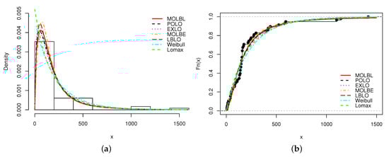
Figure 1. Plots of (a) estimated probability density function (pdf) and (b) estimated cumulative distribution function (cdf) of the MOLBL model with those of the other competitive models for Data set 1.

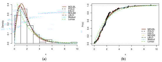
Figure 2. Plots of (a) estimated pdf and (b) estimated cdf of the MOLBL model with those of the other competitive models for Data set 2.

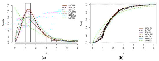
Figure 3. Plots of (a) estimated pdf and (b) estimated cdf of the MOLBL model with those of the other competitive models for Data set 3.

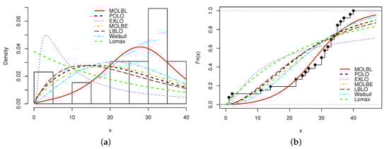
Figure 4. Plots of (a) estimated pdf and (b) estimated cdf of the MOLBL model with those of the other competitive models for Data set 4.

In all the figures, we see that the MOLBL model better adjusted the empirical objects, making enough pliancy to adapt to the right or left skewness property of the data, as well as versatile peakness.

4. Concluding Remarks

The present study completes the work of [23] about the Marshall–Olkin length-biased Lomax distribution by providing important theoretical and applied contributions. New results on the following subjects are proved: (i) compounding, (ii) stochastic ordering, (iii) asymptotic equivalences of the main functions, (iv) quantile, (v) incomplete and ordinary moments, and (vi) stress–strength parameter. Thanks to a simulation study, the maximum likelihood estimates of the parameters of the Marshall–Olkin length-biased Lomax model are proved to be numerically efficient in the convergence sense. New applications are given, revealing that the Marshall–Olkin length-biased Lomax model is more powerful than expected; it can outperform the famous power Lomax, exponentiated Lomax, Marshall–Olkin length-biased exponential, length-biased Lomax, Weibull and Lomax models. This fact is illustrated by the analysis of four different data sets coming from real-life experiments. Graphic evidence is also provided.

We hope that the present study has revealed the potential of the Marshall–Olkin length-biased Lomax distribution for various probabilistic and statistical purposes, also opening new application horizons.

References

- Lomax, K.S. Business failures: Another example of the analysis of failure data. J. Am. Stat. Assoc. 1954, 49, 847–852. [Google Scholar] [CrossRef]
- Johnson, N.L.; Kotz, S.; Balakrishnan, N. Continuous Univariate Distributions, 2nd ed.; Wiley: New York, NY, USA, 1994; Volume 1. [Google Scholar]
- Balakrishnan, N.; Ahsanullah, M. Relations for single and product moments of record values from Lomax distribution. Sankhya B 1994, 56, 140–146. [Google Scholar]
- Balkema, A.; de Haan, L. Residual life time at great age. Ann. Probab. 1974, 2, 792–804. [Google Scholar] [CrossRef]
- Bryson, M.C. Heavy-tailed distributions: Properties and tests. Technometrics 1974, 16, 61–68. [Google Scholar] [CrossRef]
- Abdullah, M.A.; Abdullah, H.A. Estimation of Lomax parameters based on generalized probability weighted moment. J. King Abdulaziz Univ. Sci. 2010, 22, 171–184. [Google Scholar]
- Afaq, A.; Ahmad, S.P.; Ahmed, A. Bayesian analysis of shape parameter of Lomax distribution under different loss functions. Int. J. Stat. Math. 2010, 2, 55–65. [Google Scholar]
- Ferreira, P.H.; Ramos, E.; Ramos, P.L.; Gonzales, J.F.B.; Tomazella, V.L.D.; Ehlers, R.S.; Silva, E.B.; Louzada, F. Objective Bayesian Analysis for the Lomax Distribution. Stat. Probab. Lett. 2020, 159, 108677. [Google Scholar] [CrossRef]
- Ahsanullah, M. Record values of Lomax distribution. Stat. Ned. 1991, 41, 21–29. [Google Scholar] [CrossRef]
- Ghitany, M.E.; Al-Awadhi, F.A.; Alkhalfan, L.A. Marshall–Olkin extended Lomax distribution and its application to censored data. Commun. Stat. Theor. Methods 2007, 36, 1855–1866. [Google Scholar] [CrossRef]
- Ashour, S.K.; Eltehiwy, M.A. Transmuted Lomax distribution. Am. J. Appl. Math. Stat. 2013, 1, 121–127. [Google Scholar] [CrossRef]
- Lemonte, A.J.; Cordeiro, G.M. An extended Lomax distribution. J. Theor. Appl. Stat. 2013, 47, 800–816. [Google Scholar] [CrossRef]
- Al-Zahrani, B.; Sagor, H. The Poisson–Lomax distribution. Rev. Colomb. Estad. 2014, 37, 225–245. [Google Scholar] [CrossRef]
- Salem, H.M. The exponentiated Lomax distribution: Different estimation methods. Am. J. Appl. Math. Stat. 2014, 2, 364–368. [Google Scholar] [CrossRef]
- El, A.H.; Abdo, N.F.; Shahen, H.S. Exponential Lomax Distribution. Int. J. Comput. Appl. 2015, 121, 24–29. [Google Scholar]
- Cordeiro, G.M.; Ortega, E.M.M.; Popović, B.V. Gamma–Lomax Distribution. J. Stat. Comput. Simul. 2015, 85, 305–319. [Google Scholar] [CrossRef]
- Tahir, M.H.; Cordeiro, G.M.; Mansoor, M.; Zubair, M. The Weibull–Lomax distribution: Properties and applications. Hacettepe J. Math. Stat. 2015, 44, 461–480. [Google Scholar] [CrossRef]
- Kilany, N.M. Weighted Lomax distribution. SpringerPlus 2016, 5, 1862. [Google Scholar] [CrossRef]
- Rady, E.H.A.; Hassanein, W.A.; Elhaddad, T.A. The power Lomax distribution with an application to bladder cancer data. SpringerPlus 2016, 5, 1838. [Google Scholar] [CrossRef]
- Ahmad, A.; Ahmad, S.P.; Ahmed, A. Length-biased weighted Lomax distribution: Statistical properties and application. Pak. Stat. Oper. Res. 2016, 12, 245–255. [Google Scholar] [CrossRef]
- Anwar, M.; Zahoor, J. The half-logistic Lomax distribution for lifetime Modeling. J. Probab. Stat. 2018, 2018, 3152807. [Google Scholar] [CrossRef]
- Haq, M.A.U.; Hamedani, G.G.; Elgarhy, M.; Ramos, P.L. Marshall–Olkin Power Lomax distribution: Properties and estimation based on complete and censored samples. Int. J. Stat. Probab. 2020, 9, 1–48. [Google Scholar]
- Mathew, J. Reliability test plan for the Marshall–Olkin length biased Lomax distribution. Reliab. Theory Appl. 2020, 15, 36–49. [Google Scholar]
- Fisher, R.A. The effects of methods of ascertainment upon the estimation of frequencies. Ann. Eugen. 1934, 6, 13–25. [Google Scholar] [CrossRef]
- Marshall, A.W.; Olkin, I. A new method for adding a parameter to a family of distributions with application to the exponential and Weibull families. Biometrica 1997, 84, 641–652. [Google Scholar] [CrossRef]
- Lee, E.T.; Wang, J.W. Statistical Methods for Survival Data Analysis, 3rd ed.; John Willey: New York, NY, USA, 2003. [Google Scholar]
- Bourguignon, M.; Silva, R.B.; Cordeiro, G.M. The Weibull-G Family of Probability Distributions. J. Data Sci. 2014, 12, 53–68. [Google Scholar]
- Shaked, M.; Shanthikumar, J.G. Stochastic Orders; Wiley: New York, NY, USA, 2007. [Google Scholar]
- Muller, A.; Stoyan, D. Comparison Methods for Stochastic Models and Risks; Wiley: Chicheste, UK, 2002. [Google Scholar]
- Boland, P.J.; El-Neweihi, E.; Proschan, F. Applications of the hazard rate ordering in reliability and order statistics. J. Appl. Probab. 1994, 31, 180–192. [Google Scholar] [CrossRef]
- Butler, R.J.; McDonald, J.B. Using incomplete moments to measure inequality. J. Econom. 1989, 42, 109–119. [Google Scholar] [CrossRef]
- Arnold, B.C. On Zenga and Bonferroni curves. Metron 2015, 73, 25–30. [Google Scholar] [CrossRef]
- Pepe, M.S. Receiver operating characteristic methodology. J. Am. Stat. Assoc. 2000, 95, 308–311. [Google Scholar] [CrossRef]
- Briggs, W.M.; Zaretzki, R. The skill plot: A graphical technique for evaluating continuous diagnostic tests. Biometrics 2008, 63, 250–261. [Google Scholar] [CrossRef]
- Church, J.D.; Harris, B. The estimation of reliability from stress-strength relationship. Technometrics 1970, 12, 49–54. [Google Scholar] [CrossRef]
- Gupta, R.C.; Ghitany, M.E.; Al-Mutairi, D.K. Estimation of reliability from Marshall–Olkin extended Lomax distributions. J. Stat. Comput. Simul. 2010, 80, 937–947. [Google Scholar] [CrossRef]
- Henningsen, A.; Toomet, O. maxLik: A package for maximum likelihood estimation in R. Comput. Stat. 2011, 26, 443–458. [Google Scholar] [CrossRef]
- Kirkpatrick, S.; Gelatt, C.D.; Vecchi, M.P. Optimization by simulated annealing. Science 1983, 220, 671–680. [Google Scholar] [CrossRef] [PubMed]
- Ramos, P.L.; Nascimento, D.C.; Ferreira, P.H.; Weber, K.T.; Santos, T.E.G.; Louzada, F. Modeling traumatic brain injury lifetime data: Improved estimators for the generalized Gamma distribution under small samples. PLOS ONE 2019, 14, e0221332. [Google Scholar] [CrossRef] [PubMed]
- Haq, M.A.U.; Usman, R.M.; Hashmi, S.; Al-Omeri, A.I. The Marshall–Olkin length-biased exponential distribution and its applications. J. King Saud Univ. Sci. 2019, 31, 246–251. [Google Scholar] [CrossRef]
- Shukla, K.K. A comparative study of one parameter lifetime distributions. Biomet. Biostat. Int. J. 2019, 8, 111–123. [Google Scholar] [CrossRef]
- Pobocikova, I.; Sedliackova, Z.; Michalkova, M. Transmuted Weibull distribution and its applications. MATEC Web Conf. 2018, 157, 08007. [Google Scholar] [CrossRef][Green Version]
- Alghamedi, A.; Dey, S.; Kumar, D.; Dobbah, S. A new extension of extended exponential distribution with applications. Ann. Data Sci. 2020, 7, 139–162. [Google Scholar] [CrossRef]
- Klein, J.P.; Moeschberger, M.L. Techniques for Censored and Truncated Data in Survival Analysis; Springer: New York, NY, USA, 1997. [Google Scholar]
Sample Availability: Samples of the compounds ...... are available from the authors. |
Publisher’s Note: MDPI stays neutral with regard to jurisdictional claims in published maps and institutional affiliations. |
© 2020 by the authors. Licensee MDPI, Basel, Switzerland. This article is an open access article distributed under the terms and conditions of the Creative Commons Attribution (CC BY) license (http://creativecommons.org/licenses/by/4.0/).