
An Intelligent Process Fault Diagnosis System Based on Neural Networks and Andrews Plot


School of Engineering, Merz Court, Newcastle University, Newcastle upon Tyne NE1 7RU, UK
*
Author to whom correspondence should be addressed.
Processes 2021, 9(9), 1659; https://doi.org/10.3390/pr9091659
Submission received: 7 August 2021
/
Revised: 3 September 2021
/
Accepted: 9 September 2021
/
Published: 14 September 2021
(This article belongs to the Special Issue Redesign Processes in the Age of the Fourth Industrial Revolution)
Abstract
:This paper proposes a neural network-based process fault diagnosis system with Andrews plot for information pre-processing to enhance the performance of online process fault diagnosis. By using features extracted from Andrews plot as the inputs to a neural network, as a classifier, the diagnosis speed and reliability are improved. A method for determining the important features in the Andrews function is proposed. The proposed fault diagnosis system is applied to a simulated continuous stirred tank reactor process and is compared with two conventional neural network-based fault diagnosis systems: scheme B where the monitored measurements are directly fed to a neural network after scaling and scheme C where the monitored measurements are converted to qualitative trend data before feeding to a neural network. Of all the considered faults, the proposed fault diagnosis system diagnosed the abrupt faults on average 5.45 s and 2.66 s earlier than schemes B and C, respectively and diagnosed the incipient faults on average 13.82 s and 5.09 s earlier than schemes B and C, respectively. The results reveal that Andrews plot method utilized in online process monitoring has a great potential in industrial process monitoring.
1. Introduction
The breakthroughs and advances in industrial technology have made modern industrial production processes more automatic and productive with complex operational functionalities. These improvements have enhanced the product quality and expanded the production scale during the past decades. The associated risk of potential failures of various components increases with the complexity and functionality of modern industrial processes. Any faults hidden in insignificance could potentially lead to colossal damages if they remain undetected. Faults are hard to be completely eliminated in chemical industry. Undetected faults in an industrial production process could be accompanied by large hidden risks, which will cause distressingly serious consequences and the subsequent indirect impacts. Degradation in product quality, as a quintessentially consequence, can ruin the brand reputation and corporate identity. Particularly to small-and-medium-sized enterprises, this perhaps can lead to capital chain rupture and disrupt the development of the enterprise. Environmental contamination is also a typical effect of chemical process accidents. Authoritativeness of local authorities may be challenged due to the duty of environmental conservation and enterprises may also risk heavy penalties. Disastrous consequences, such as casualties, usually bring inestimable lost, which should be completely avoided. Generally, with the advancement of industrial technology, the improvement of social environmental awareness and the increased demand for high-quality products, the importance of industrial process monitoring is becoming increasingly important. This paper aims to propose a novel fault diagnosis system to achieve a positive promotion in industrial process monitoring.
The various proposed fault detection and diagnosis approaches can broadly be classified into the following three main approaches: model-based approaches, knowledge-based approaches and data analysis-based approaches [1,2,3,4]. Currently, big data analytics and machine learning are popularly used in developing new fault diagnosis techniques. Previous works give plenty of diagnosis strategies based on multivariate statistical data analysis [5,6]. Qin [7] gave a detailed survey on data-driven industrial process monitoring and diagnosis using multivariate statistical data analysis techniques. Ge [8] reviewed data-driven modelling and monitoring techniques for plant-wide industrial processes. Wang et al. [9] reviewed theoretical research and engineering applications of multivariate statistical process monitoring algorithms for the period 2008–2017. Multitudinous positive research works evidenced that various neural networks, as an excellent classifier, can provide helpful fault diagnosis results in online process monitoring. Zhang and Morris [10] presented a fuzzy neural network for on-line process fault diagnosis where the on-line measurements are converted into fuzzy sets in the fuzzification layer of the fuzzy neural network. Zhang [11] presented using multiple neural networks to improve the fault diagnosis performance and different approaches for aggregating multiple neural networks were investigated. Jiang et al. [12] presented using deep learning for the fault diagnosis of rotating machinery. Li et al. [13] presented an approach for nonlinear industrial process fault diagnosis using autoencoder embedded dictionary learning. Li et al. [14] integrated wavelet transform with convolutional neural network for the monitoring of a large-scale fluorochemical process. The advantage of using neural networks is that the multiple independent and dependent variables can be handled synchronously by the neural network, without the need of deep knowledge on the process such as mechanistic models [15,16]. Process modelling and fault diagnosis using the latest development of neural networks, such as the gated recurrent neural network [17], deep belief networks [18] and autoencoder gated recurrent neural network [19], have also been reported recently.
Hybrid diagnosis strategy combining neural network with multivariate statistical analysis techniques also has positive impacts on process industries [20]. Wen and Xu [21] integrated ReliefF, principal component analysis and deep neural network for the fault diagnosis of a wind turbine. Shang et al. [22] presented using slow feature analysis for soft sensor development from process operation data. Yu and Zhang [23] presented a manifold regularized stacked autoencoder-based feature learning approach for industrial process fault diagnosis. Chen et al. [24] presented using one-dimensional convolutional auto-encoder based feature learning for the fault diagnosis of multivariate processes. Bao et al. [25] presented a combined deep learning approach for chemical process fault diagnosis.
A neural network-based fault diagnosis system is typically constituted by two sub-systems. The first is a data pre-processing system to extract relevant features from online monitoring measurements, via mathematical approaches, mainly the multivariate statistical data analysis techniques. Another is a process state analysis system to obtain the diagnosis results via a classifier, generally a neural network, to handle the multi-dimensional data. Using extracted features as the neural network inputs would help the neural network in classifying the various faults than directly using the monitored process measurements as the neural network inputs. This paper intends to explore the effectiveness of Andrews plot in extracting effective features for enhanced on-line process fault diagnosis.
The proposed data-driven intelligent fault diagnosis strategy in this paper is based on a neural network as the classifier and integrates Andrews plot to preliminarily process the monitoring information with the purpose of accelerating the diagnosis speed and enhancing the reliability of fault diagnosis. Andrews plot is a very useful visualization method for analyzing multivariate data. It has been applied to many areas including analyzing data from the 2001 Parliamentary General Election in the United Kingdom [26,27]. Its unique advantage includes the convenience in setting the dimension of the extracted feature space. Andrews plot is efficient in dealing with the issues with large number of correlated variables. A difficulty with Andrews plot is that the proper selection of the number of features. Nevertheless, Andrews plot has a great potential for improving fault detection and diagnosis performance through extracting useful features from the original monitored process measurements. This paper presents a method for determining the important features in Andrews function which give good separations between classes. The proposed fault diagnosis method is applied to a simulated continuous stirred tank reactor (CSTR) system. In order to demonstrate its superiority, it is compared with two traditional neural network-based diagnosis schemes.
The paper is organized as follows. Section 2 presents the proposed diagnosis system and details of parameter selection. Section 3 introduces the case study, a CSTR system and two traditional neural network-based fault diagnosis schemes. Section 4 presents the comparison of diagnosis performance. The determination of important features is also demonstrated. Section 5 concludes the paper.
2. The Proposed Fault Diagnosis System
2.1. Andrews Plot
Andrews plot is a visualization method for high-dimensional data originally proposed by the statistician David F. Andrews [28]. In this method, each sample of an -dimensional data set, is mapped into a curve using the following function:
where is in the range [−π, π]. Through the above function, each data sample is converted into a curve in the interval [−π, π]. In addition to the above function, Andrews [28] also suggested other functions as the following to be used in the curves.
where are different integers and t is in the range [−π, π].
In prior works, several variations to the functions of Andrews plot were proposed by some researchers such as the following functions suggested in [27,29,30], respectively:
where is in the range [−π, π] and the values of are mutually irrational and scaled between 0.5 and 1.
Utilizing the Andrews function to process information, the dimension of data can be changed to an appropriate dimension, by selecting a number of features in Andrews function, i.e., the number of t-values. In chemical process monitoring applications, multi-variable measurements are converted into an information-containing feature matrix via an Andrews function with a certain number of t-values.
2.2. The Proposed Fault Diagnosis System
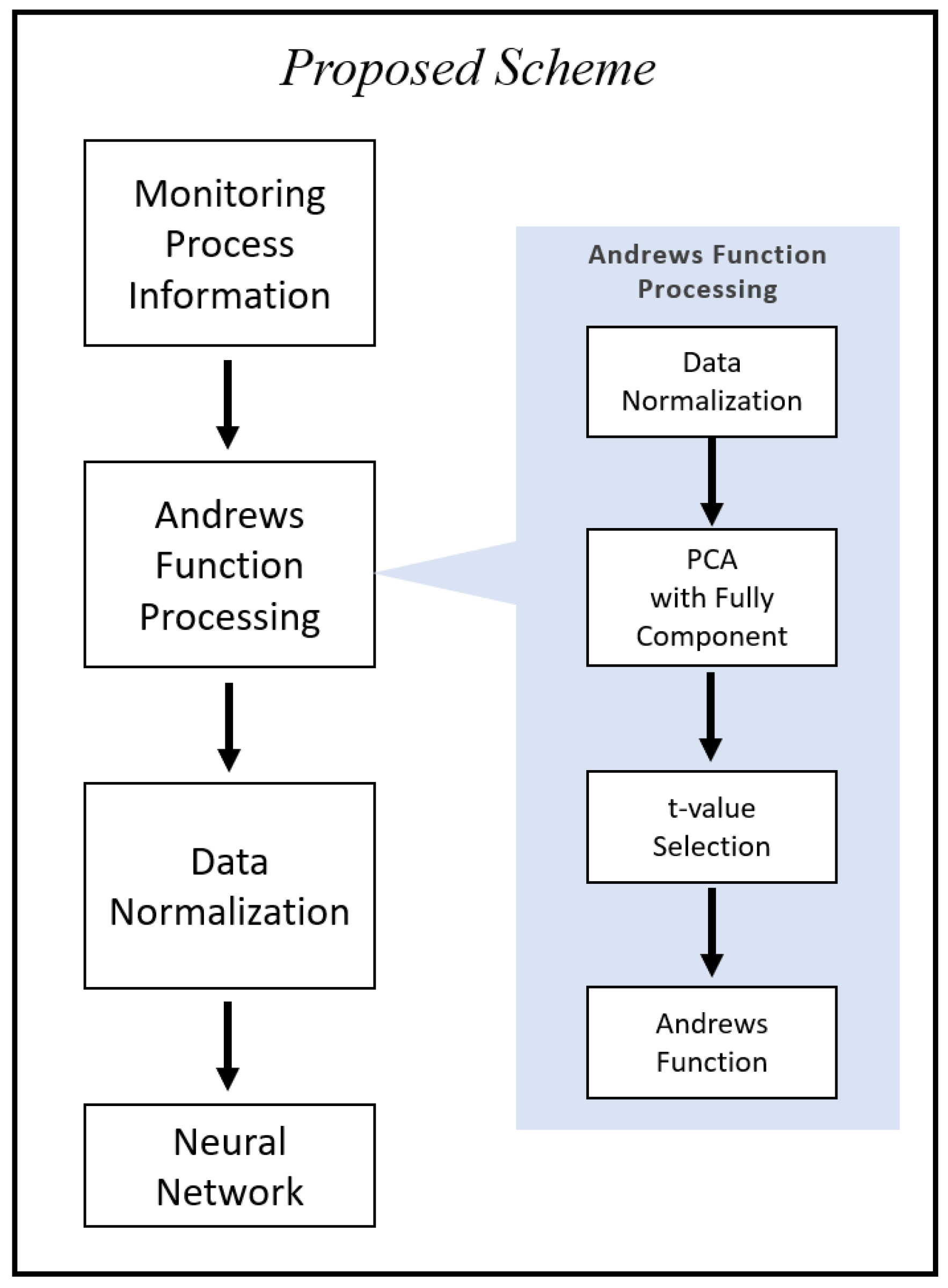
In this paper, the proposed fault diagnosis system (referred to as scheme A) includes two subsystems: data pre-processing subsystem and process state analysis subsystem. In the data pre-processing subsystem, Andrews function is used to pre-process the online measurements. The processed features are fed into process state analysis system, which is a neural network-based classifier. Figure 1 shows the framework of the proposed fault diagnosis system. Through the data pre-processing system, features are extracted from the online monitoring information. The dimension of the extracted features is given by the numbers of t-values in the Andrew function. The system uses the principal components instead of the original variables to eliminate the effects of variable ordering in the Andrew function. Then Andrews function given by Equation (1) with the selected t-values is used to obtain the information-containing feature dataset. Finally, the pre-processed features are used to train a neural network as a fault classifier.
The reason of using principal components in place of the original variables is as follows. Previous studies have shown that the multi-variable information processed by Andrews curve is highly sensitive to the ordering of variables in the data set, which can result in uncertainties [31,32]. In order to subside the effect of variable ordering on the outputs of Andrews function, principal components of the original data set are used as the inputs to Andrews function instead of the original variables [31,32]. An example to illustrate the effect of variable ordering will be given in Section 3.
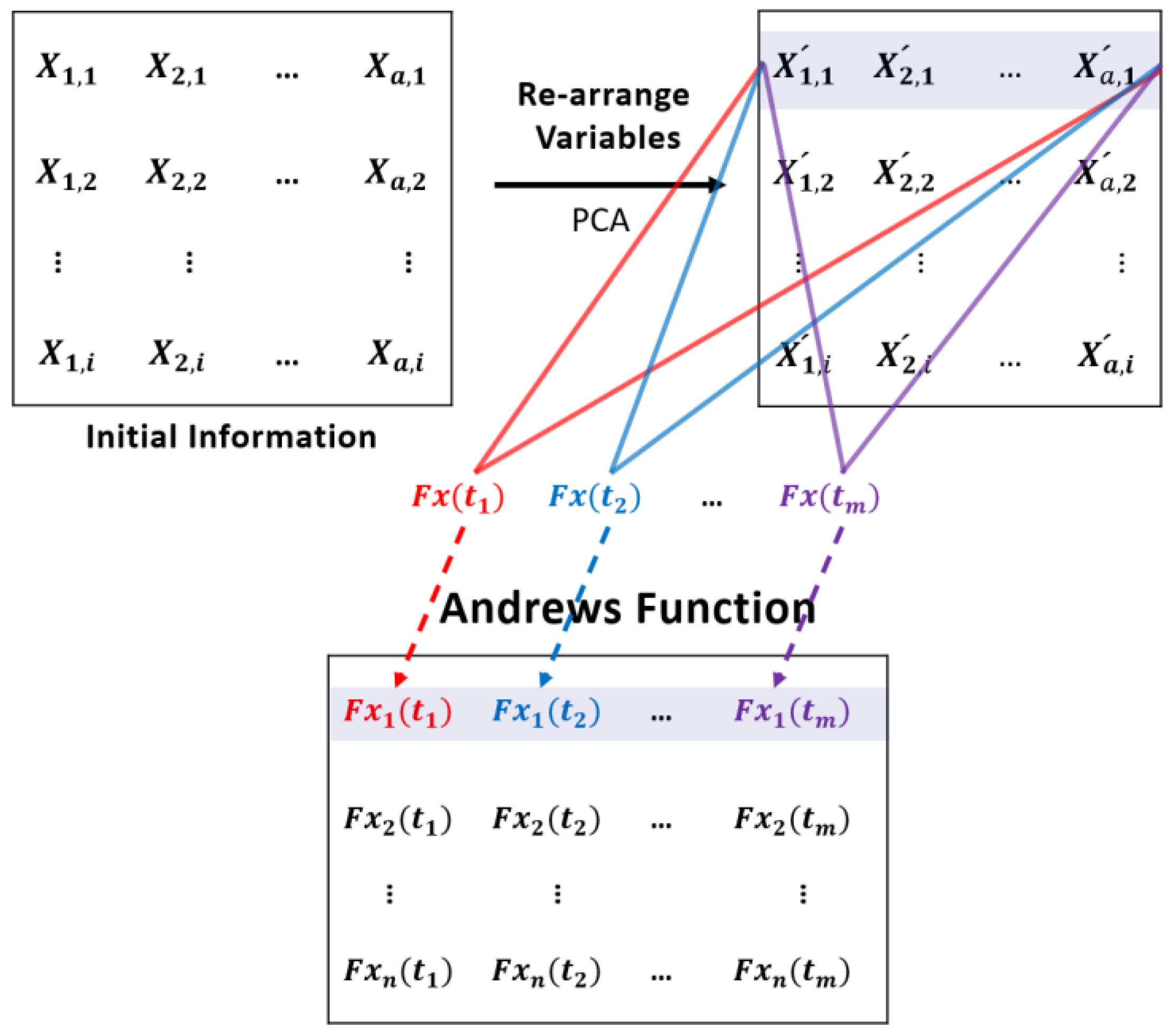
Figure 2 shows the procedure of Andrews function processing of the original data. In the proposed diagnosis scheme, an a-dimensional process data set, , is first scaled to zero mean and unit variance and then principal component analysis (PCA) is applied to the scaled data. All the principal components are used as the inputs to Andrews function with n t-values. A method for selection of the t-values (features) will be discussed later in this section. After Andrews function pre-processing, the dimension of the data is changed to n, which is the number of t-values used.
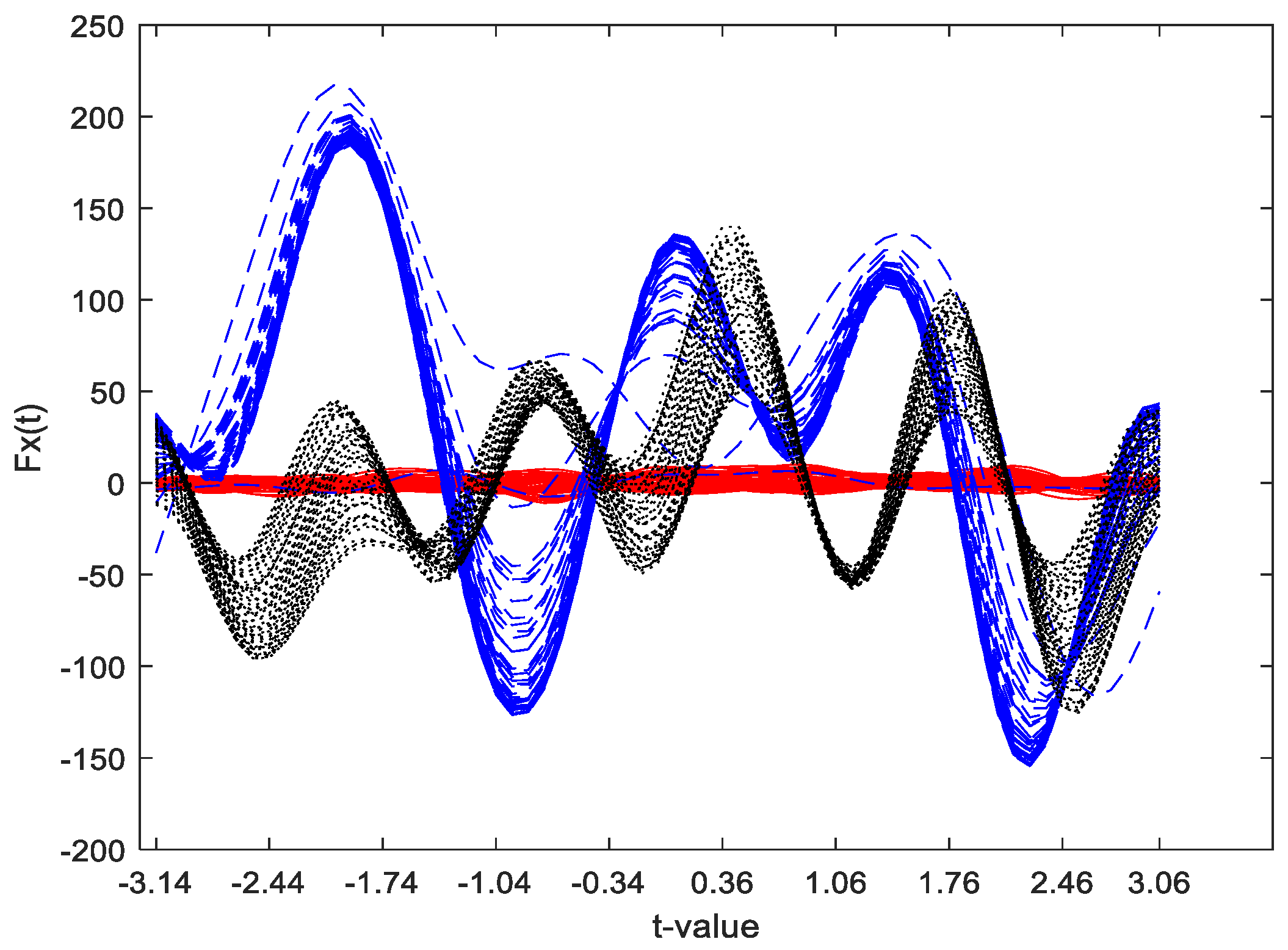
Figure 3 shows an example of Andrews plot using Equation (1) with 63 values of t uniformly distributed in the range [−π, π]. In Figure 3, the red solid curves represent the normal data, the blue dashed curves represent the data with fault No. 3 and the black dotted curves represent the data with fault No. 5. Figure 3 contains 50 samples from each class and each sample is shown as a curve calculated using Equation (1). Noted that in practice the appropriate number of t-values should properly selected. Here the 63 t-values are just used for clear visualization to observe the separations. It can be seen from Figure 3 that the monitoring information pre-processed by Andrews function can have more separations between normal data and fault data in certain values of t. This can ease the classification task leading to improved fault diagnosis performance.
It can be seen from Figure 3 that some values of t give better separations among the classes than other values. A method for determining the t-values is proposed in this paper as follows. First, using the Andrews function to process the data with a relatively large number (e.g., 100) of t-values, which are uniformly distributed in the range [−π, π]. Note here 100 is considered as sufficiently large number of t-values. Second, averaging the resulting Andrew function values at each t-value for each category (i.e., normal, fault No. 1, fault No. 2, …). Third, calculate the minimal distance among these Andrew function values at each t-value. Finally, select the first a few t-values with large minimal distance values, which indicate good separations among the classes.
3. A CSTR System
3.1. A Simulated Continuous Stirred Tank Reactor System
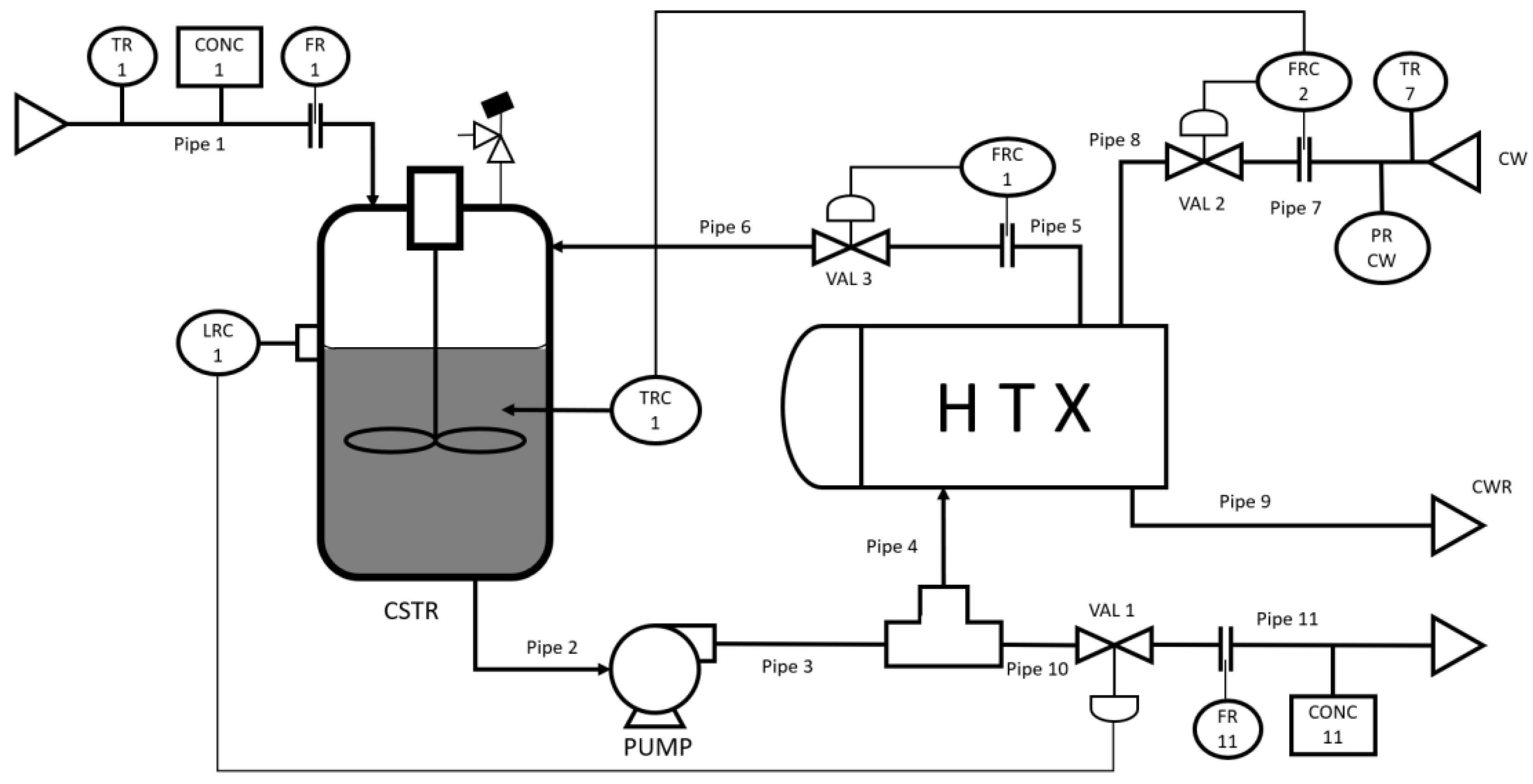
In order to demonstrate the advantages of the proposed fault diagnosis strategy, a simulated CSTR system, which is taken from [33], is used to demonstrate and compare diagnosis performance. Figure 4 shows the diagram of the CSTR system. An irreversible heterogeneous catalytic exothermic reaction takes place in the CSTR. The product concentration is indirectly maintained at a desired level by controlling temperature, residence time and mixing conditions in the CSTR. Part of the reactor outlet stream is recycled to the reactor through a heat exchanger to provide temperature control by manipulating the flow rate of the cold water fed to the heat exchanger via a cascade control system. The residence time is controlled through the reactor level controller and the mixing condition is controlled by maintaining the recycle flow rate. Constant physical properties and constant boundary pressures of all input and output streams are assumed. Perfect mixing in the reactor is assumed. Under these assumptions, a mechanistic model is developed from mass balance and energy balance and is used to simulate the process.
The simulated process measurements are generated under the normal condition and various abnormal conditions with typical measurement noise. The simulated online measurements are composed of 10 online measured process variables and 3 controller outputs. The sampling time of controllers is 4 s. Table 1 shows the 11 considered faults which are typical faults in industrial processes [33]. Table 2 shows the measurement noise ranges.
An example is given here to illustrate how the feature extraction is affected by variable ordering. Figure 5 shows Andrews plots using data under Fault No. 7 with three different process variable ordering. The 13 online information sources, , represent the 10 measured variables in the simulated CSTR system, which are temperature of input reactant, temperature in reactor, tank level, flow rate of input reactant, flow rate of recycled reactant, flow rates of product, flow rates of cold-water entering the heat exchanger, concentration of product in the reactor, concentration of the reactant in the input stream, pressure of liquid leaving the pump and 3 controller outputs.
Variable ordering No. 1 is , variable ordering No. 2 is and variable ordering No. 3 is . The left column of Figure 5 shows the results using the principal components instead of the scaled original monitoring information and the right column shows the results using the scaled original monitoring information. Note that the original monitoring information is scaled to zero mean and unit variance before applying PCA and Andrews function. The top plots (red curves) represent variable ordering No. 1, the middle plots (blue curves) represent variable ordering No. 2, and the bottom plots (black curves) represent variable ordering No. 3. The curves are produced using 100 t-values uniformly distributed in the range [−π, π] and 50 samples of the original data. From Figure 5, it can be seen that Andrews plots from the original measurements can give different results for different variable orderings. However, Andrews plots from the principal components can obviously eliminate the impacts of variable ordering. Note that the principal components are always arranged in the order of the data variance that they explained.
3.2. Baseline Fault Diagnosis Scheme in CSTR System
In this paper, a conventional neural network-based fault diagnosis system is developed as a comparative study. In this baseline diagnosis scheme (referred to as scheme B), the original measurements are scaled and then directly fed into a neural network. To generate the data used for neural network training and testing, normal operation data and faulty operation data for each fault in the form of abrupt fault are generated from simulation. Table 3 gives the variable values corresponding to the 11 faults. These values are utilized in the simulated CSTR system to generate the considered fault dataset for neural network training. Figure 6 shows the baseline scheme. The scaling equation in this case is given by the following:
where is the actual value, is pre-processed values for the th on-line measurement, is the mean value of normal data and is the standard deviation of normal data.
In addition to this baseline scheme, another scheme (referred to as scheme C) is also used to compare with the proposed scheme. In scheme C, the monitored process information (xi) is converted into qualitative trend values (xi,p): increase (1), steady (0) and decrease (−1) as follows:
where σi is the standard deviation of the ith measurement under a normal operating condition.
3.3. Abrupt Faults and Incipient Faults in the CSTR System
In this paper, both abrupt faults and incipient faults are considered. An abrupt fault means that the process parameter related to the fault varies suddenly when the fault occurs. An abrupt fault is simulated as a step change in the associated process parameter. An incipient fault means that the fault magnitude is gradually growing. At the early stage of an incipient fault, its effect is hidden in trifle and then it will cumulate sufficient damages if it remains undetected. The growth of an incipient fault can be described by the following equation:
where is the normal value of a process parameter, represents the faulty value of the same process parameter at time , is the fault developing speed of an incipient fault and is the time from the initiation of the incipient fault. The above equation can be used to represent common incipient faults in industrial processes [33].
In this study, three groups of abrupt faults and three groups of incipient faults under different fault conditions were generated as unseen validation data for evaluating the developed fault diagnosis systems. Table 4 gives three groups of relative fault magnitudes (Mag. 1, Mag. 2 and Mag. 3) corresponding to the 11 abrupt faults. Table 5 gives three groups of fault developing speeds (γ1, γ2 and γ3) corresponding to the 11 incipient faults.
4. Results
4.1. Fault Diagnosis System Development
The performance of the proposed diagnosis scheme A is compared with the conventional schemes B and C under abrupt faults and incipient faults. In the proposed scheme A, the selection of t values (the number of features) in Andrews function is important and can affect the final diagnosis performance. In practical application, since the infinite number of t-value in Andrews function and large number of variables in a chemical engineering process, the selection of appropriate t-values may be time consuming.
The method for determining the important features (t-values) presented in Section 2 is used here. Andrew function values for all the data at 100 t-values uniformly distributed in the range [−π, π] are calculated. The minimum distance between all the classes (normal, fault No. 1, …, fault No. 11) is calculated at each of these t-values. Figure 7 shows the top 30 minimal distance values in descending order. It can be seen that the minimal distance values drop quickly after about the first 11 t-values. Therefore, the first 11 t-values are selected, i.e., the final selected values of t are [−3.1414, −0.6846, −0.5586, −0.4956, −0.4326, −0.3696, 0.2604, 2.9064, 209694, 3.3024, 3.0954].
The training and testing data were produced using simulation based on the mechanistic model of the process. Simulated process operational data under the normal operation and the 11 faults with the fault conditions given in Table 3 were generated. For each fault, 80 samples were collected when one or more of the process variables exist 3 times of their normal standard deviations. The normal operation data also contains 80 samples. For the 80 samples corresponding to each category, 50 samples were randomly selected as training data while the remaining 30 samples were used as the testing data. Thus, the training data set contains 600 samples and the testing data sets contains 360 samples. The neural networks were trained on the training data set and the testing data set was used for network structure determination and implementing the “early stopping” mechanism during network training [15]. In all the three schemes, the neural networks are single hidden layer feedforward networks with sigmoid function in the hidden layer and output layer. All networks have 11 output layer neurons corresponding to the 11 faults. The networks were trained using the backpropagation training method with the learning rate, momentum constant and maximum training steps selected as 0.01, 0.9 and 1000, respectively. The training objective is to minimize the mean squared errors of the network. During network training, a target output of 1 is assigned to the network output corresponding to the fault while the targets for other network outputs are 0. During diagnosis, the neural network outputs should be lower than 0.2 when the samples are under the normal operating condition. A diagnosis result is issued when the neural network output corresponding to the fault is higher than 0.8 while other network outputs are below 0.2. An advance warning is issued when the neural network output corresponding to the fault is higher than 0.4. Evaluation of fault diagnosis systems is mainly based on accuracy, robustness and speed of diagnosis. The diagnosis time is measured as the time between a fault being initiated and being successfully diagnosed. The advance warning time is defined as the time between the fault being initiated and a correct advance warning being issued.
The number of hidden neurons was determined through cross validation on the testing data. A number of neural networks with different numbers of hidden neurons were trained on the training data and tested on the testing data. The network gives the overall best performance on the testing data is considered as having the appropriate number of hidden neurons. Table 6, Table 7 and Table 8 give the accuracy of different numbers of hidden neurons in diagnosis schemes A, B and C on the testing data, respectively. In Table 6, Table 7 and Table 8, the best performance is marked with bold font. It can be seen that the best numbers of hidden neurons for schemes A, B and C are 15, 17 and 13, respectively. Table 9 summarizes the numbers of neurons in different layers of the neural networks.
4.2. Performance under Abrupt Faults
The proposed scheme A and the conventional schemes B and C are tested on three groups of abrupt faults given by Table 4 to demonstrate the superiorities of the proposed method. All of the abrupt faults were initiated at 40 s. Table 10 indicates that all diagnosis systems successfully diagnosed all the considered abrupt faults. In terms of diagnosis speed, the proposed diagnosis scheme A diagnosed the abrupt faults 5.45 s and 2.66 s earlier on average than schemes B and C, respectively. Note that as the sampling time is given, traditional metrics such as the fault detection rate (FDR) and the missed detection rate (MDR) can be easily obtained from the fault diagnosis times given in Table 10. Table 11 gives the FDR for abrupt faults. In all the considered faults here, there are no incorrect diagnosis cases and the undetected samples are during the early stages of the faults. Thus, for all the considered faults here, MDR can be simply obtained as 1-FDR. It can be seen from Table 11 that the proposed scheme A gives overall higher FDR than schemes B and C. Table 11 also indicates that the FDR is higher when the fault magnitude is higher as a fault with higher magnitude is generally easier to detect and diagnosis than the same fault with lower magnitude. Figure 8 and Figure 9 show two sets of diagnosis outputs in abrupt faults as examples to show the robustness of the proposed scheme.
Figure 8 shows the performance of schemes A and B in diagnosing abrupt fault No. 2, with the fault relative magnitude being 1.67%. In Figure 8 and the subsequent diagnosis output plots, F1 to F11 represent the neural network outputs corresponding to Fault No. 1 to No. 11 listed in Table 1, respectively. The upper dash-dotted lines indicate the diagnosis threshold (0.8) while the lower dash-dotted lines indicate the advance warning threshold (0.4). Figure 8a shows that scheme A successfully diagnosed the fault at 20 s after the fault being initiated. Figure 8b shows that the outputs from scheme B responded quickly, when the abnormal condition occurred but with fluctuations. Eventually the fault was diagnosed at 32 s after the fault being initiated. The output curve then still oscillates with a certain magnitude over the 0.8. It can be seen that the proposed scheme A diagnosed the fault 12 s earlier than scheme B and the output curve is steadier than scheme B.
Figure 9 shows the performance of schemes A and B in diagnosing abrupt fault No. 7, with the fault relative magnitude being 27.86%. As in the previous case, the outputs in scheme A have isolated points exceeding the diagnosis threshold (0.8) before the oscillation stabilized. Figure 9a shows that scheme A successfully diagnosed the fault at 16 s after the fault being initiated. Figure 9b shows that scheme B successfully diagnosed the fault at 36 s after fault being initiated. The diagnosis time of scheme A for this fault is 20 s shorter than that of scheme B.
4.3. Performance under Incipient Faults
The proposed scheme A and the conventional schemes B and C are applied to three groups of incipient faults given by Table 5 to compare fault diagnosis results. All of the incipient faults were initiated at 0 s. Table 12 indicates that all diagnosis systems successfully diagnosed all the considered incipient faults. In terms of the diagnosis speed, the proposed diagnosis scheme A diagnosed the incipient faults 13.82 s and 5.09 s earlier on average than schemes B and C, respectively. Table 13 gives the FDR values for the considered incipient faults of the three schemes. In can be seen that the proposed scheme A gives overall higher FDR than schemes B and C. Table 13 also indicates that the FDR is higher when the fault developing speed is higher as a faster developing fault is generally easier to detect and diagnosis than a slower developing fault. As with the abrupt fault cases, there are no incorrect diagnosis cases and all the undetected samples are during the early stages of the faults when their magnitudes are low. Thus, MDR can be simply worked out as 1-FDR and are not shown here. The following figures show three sets of diagnosis outputs in incipient faults as examples to show the good performance of the proposed scheme.
Figure 10 shows the performance of scheme A and scheme B in diagnosing incipient fault No. 3, with the fault developing speed as . It can be seen from Figure 10a that, under scheme A, the network output corresponding to fault No. 3 raises to over 0.8 with some slight oscillations after a period fault developing, while all other network outputs remain close to 0. As shown in Figure 10b, under scheme B, the network output corresponding to fault No. 3 gradually raises accompanied with some large oscillations until across the diagnosis threshold, then it becomes steady, while all other network outputs remain close to 0. Hence, both schemes successful diagnosed fault No. 3 occurred in this process. Figure 10a shows that scheme A successfully diagnosed the fault at 104 s. Figure 10b shows that scheme B successfully diagnosed the fault at 152 s. For this particular incipient fault, scheme A diagnosed the fault 48 s earlier than scheme B, and the output curves of scheme A also stabilize earlier than those of scheme B.
Figure 11 shows the performance of schemes A and B in diagnosing incipient fault No. 5, with the fault developing speed being . As shown in Figure 11a, after the period of fault progressing, the network output corresponding to fault No. 5 raises up and exceeds 0.8 rapidly, while all other network outputs remain close to 0. Hence, scheme A successfully diagnosed the fault at 116 s. As shown in Figure 11b, the network output corresponding to fault No. 5 gradually increases across the diagnosis threshold 0.8, while all other network outputs remain close to 0. Hence, scheme B successfully diagnosed the fault at 152 s. For this particular incipient fault, the proposed scheme A diagnosed the fault 36 s earlier than scheme B, and the output curves of scheme A also stabilize earlier than those of scheme B.
Figure 12 shows the performance of schemes A and B in diagnosing incipient fault No. 10, with the fault developing speed being . It can be seen from Figure 12 that, after an initial period of fault progressing, the network output corresponding to fault No. 10 gradually increases close to 1 with some slight oscillations, while all other network outputs remain lower than 0.2. Figure 12a shows that scheme A successfully diagnosed the fault at 96 s. Figure 12b shows that scheme B successfully diagnosed the fault at 124 s. It can be seen that the output curve corresponding to fault No. 10 from scheme B is slower in reaching the diagnosis threshold when the abnormal condition occurred. In this case, the proposed scheme A diagnosed the fault 28 s earlier than scheme B.
5. Conclusions
This paper proposes an enhanced intelligent neural network based online process fault diagnosis system by integrating Andrews plot and neural network techniques. By using features extracted from Andrews plot as the inputs to a neural network, the diagnosis speed and reliability are improved. A method for determining the important features in Andrews function is also proposed. Applications to a simulated CSTR process show very encouraging results. It is shown that the proposed method can give good performance in terms of diagnosis speed and accuracy. In addition, the proposed data pre-processing method is highly effective in adjusting the high dimensional data to an appropriate size. As with other neural network-based fault diagnosis systems, one limitation of the proposed method is that it requires the availability of process data covering various faults. Coping with imbalanced data sets and unavailability of certain fault data deserves future investigation. Integrating Andrews plot with other machine learning methods such as support vector machines or random forests could be carried out in the future. Furthermore, the combined use of Andrew plot and other feature extraction approaches could be investigated in the future to reduce uncertainty. Applications to real-world systems could be considered in the future.
Author Contributions
Conceptualization, S.W. and J.Z.; methodology, S.W. and J.Z.; software, S.W. and J.Z.; validation, S.W.; formal analysis, S.W.; investigation, S.W.; resources, J.Z.; data curation, S.W. and J.Z.; writing—original draft preparation, S.W.; writing—review and editing, J.Z.; visualization, S.W.; supervision, J.Z.; project administration, J.Z.; funding acquisition, J.Z. Both authors have read and agreed to the published version of the manuscript.
Funding
This research was funded by the EU (Project No. PIRSES-GA-2013-612230) and National Natural Science Foundation of China (61673236).
Institutional Review Board Statement
Not applicable.
Informed Consent Statement
Not applicable.
Conflicts of Interest
The authors declare no conflict of interest.
References
- Venkatasubramanian, V.; Rengaswamy, R.; Yin, K.; Kavuri, S.N. A review of process fault detection and diagnosis: Part I: Quantitative model-based methods. Comput. Chem. Eng. 2003, 27, 293–311. [Google Scholar] [CrossRef]
- Venkatasubramanian, V.; Rengaswamy, R.; Kavuri, S.N. A review of process fault detection and diagnosis: Part II: Qualitative models and search strategies. Comput. Chem. Eng. 2003, 27, 313–326. [Google Scholar] [CrossRef]
- Venkatasubramanian, V.; Rengaswamy, R.; Kavuri, S.N.; Yin, K. A review of process fault detection and diagnosis: Part III: Process history based methods. Comput. Chem. Eng. 2003, 27, 327–346. [Google Scholar] [CrossRef]
- Zhang, J.; Roberts, P. Process fault diagnosis with diagnostic rules based on structural decomposition. J. Process. Control. 1991, 1, 259–269. [Google Scholar] [CrossRef]
- MacGregor, J.; Kourti, T. Statistical process control of multivariate processes. Control. Eng. Pr. 1995, 3, 403–414. [Google Scholar] [CrossRef]
- Zhang, J.; Martin, E.B.; Morris, A.J. Fault-detection and diagnosis using multivariate statistical techniques. Chem. Eng. Res. Des. 1996, 74, 89–96. [Google Scholar]
- Qin, S.J. Survey on data-driven industrial process monitoring and diagnosis. Annu. Rev. Control. 2012, 36, 220–234. [Google Scholar] [CrossRef]
- Ge, Z. Review on data-driven modeling and monitoring for plant-wide industrial processes. Chemom. Intell. Lab. Syst. 2017, 171, 16–25. [Google Scholar] [CrossRef]
- Wang, Y.; Si, Y.; Huang, B.; Lou, Z. Survey on the theoretical research and engineering applications of multivariate statistics process monitoring algorithms: 2008–2017. Can. J. Chem. Eng. 2018, 96, 2073–2085. [Google Scholar] [CrossRef]
- Zhang, J.; Morris, A.J. Process modelling and fault diagnosis using fuzzy neural networks. Fuzzy Sets Syst. 1996, 10, 313–326. [Google Scholar] [CrossRef]
- Zhang, J. Improved on-line process fault diagnosis through information fusion in multiple neural networks. Comput. Chem. Eng. 2006, 30, 558–571. [Google Scholar] [CrossRef]
- Jiang, W.; Wang, C.; Zou, J.; Zhang, S. Application of deep learning in fault diagnosis of rotating machinery. Processes 2021, 9, 919. [Google Scholar] [CrossRef]
- Li, Y.; Chai, Y.; Yin, H. Autoencoder embedded dictionary learning for nonlinear industrial process fault diagnosis. J. Process. Control. 2021, 101, 24–34. [Google Scholar] [CrossRef]
- Li, X.; Zhou, K.; Xue, F.; Chen, Z.; Ge, Z.; Chen, X.; Song, K. A wavelet transform-assisted convolutional neural network multi-model framework for monitoring large-scale fluorochemical engineering processes. Processes 2021, 8, 1480. [Google Scholar] [CrossRef]
- Bishop, C.M. Neural Networks for Pattern Recognition; Oxford University Press, Inc.: Oxford, UK, 1995. [Google Scholar]
- Venkatasubramanian, V.; Chan, K. A neural network methodology for process fault diagnosis. AIChE J. 1989, 35, 1993–2002. [Google Scholar] [CrossRef]
- Ouyang, H.; Zeng, J.; Li, Y.; Luo, S. Fault detection and identification of blast furnace ironmaking process using the gated recurrent unit network. Processes 2020, 8, 391. [Google Scholar] [CrossRef] [Green Version]
- Zhu, C.-H.; Zhang, J. Developing soft sensors for polymer melt index in an industrial polymerization process using deep belief networks. Int. J. Autom. Comput. 2020, 17, 44–54. [Google Scholar] [CrossRef] [Green Version]
- Lu, Y.-W.; Hsu, C.-Y.; Huang, K.-C. An autoencoder gated recurrent unit for remaining useful life prediction. Processes 2020, 8, 1155. [Google Scholar] [CrossRef]
- Ramezani, J.; Jassbi, J. Quality 4.0 in action: Smart hybrid fault diagnosis system in plaster production. Processes 2020, 8, 634. [Google Scholar] [CrossRef]
- Wen, X.; Xu, Z. Wind turbine fault diagnosis based on ReliefF-PCA and DNN. Expert Syst. Appl. 2021, 178, 115016. [Google Scholar] [CrossRef]
- Shang, C.; Huang, B.; Yang, F.; Huang, D. Probabilistic slow feature analysis-based representation learning from massive process data for soft sensor modeling. AIChE J. 2015, 61, 4126–4139. [Google Scholar] [CrossRef]
- Yu, J.; Zhang, C. Manifold regularized stacked autoencoders-based feature learning for fault detection in industrial processes. J. Process Control 2020, 92, 119–136. [Google Scholar] [CrossRef]
- Chen, S.; Yu, J.; Wang, S. One-dimensional convolutional auto-encoder-based feature learning for fault diagnosis of multivariate processes. J. Process Control 2020, 87, 54–67. [Google Scholar] [CrossRef]
- Bao, Y.; Wang, B.; Guo, P.; Wang, J. Chemical process fault diagnosis based on a combined deep learning method. Can. J. Chem. Eng. 2021. [Google Scholar] [CrossRef]
- Spencer, N.H. Investigating data with Andrews plots. Soc. Sci. Comput. Rev. 2003, 21, 244–249. [Google Scholar] [CrossRef] [Green Version]
- Khattree, R.; Naik, D.N. Andrews plots for multivariate data: Some new suggestions and applications. J. Stat. Plan. Inference 2002, 100, 411–425. [Google Scholar] [CrossRef]
- Andrews, D.F. Plots of high-dimensional data. Biometrics 1972, 28, 125. [Google Scholar] [CrossRef]
- Kulkarni, S.; Paranjape, S. Use, of Andrews’ function plot technique to construct control curves for multivariate process. Commun. Stat. Theory Methods 1984, 13, 2511–2533. [Google Scholar] [CrossRef]
- Wegman, E.J.; Shen, J. Three-dimensional Andrews plots and the grand tour. Comput. Sci. Stat. 1993, 25, 284–288. [Google Scholar]
- Moustafa, R.E. Andrews curves. Wiley Interdiscip. Rev. Comput. Stat. 2011, 3, 373–382. [Google Scholar] [CrossRef]
- Boonprong, S.; Cao, C.; Torteeka, P.; Chen, W. A novel classification technique of Landsat-8 OLI image-based data visualization: The application of Andrews’ plots and fuzzy evidential reasoning. Remote Sens. 2017, 9, 427. [Google Scholar] [CrossRef] [Green Version]
- Zhang, J.; Roberts, P. On-line process fault diagnosis using neural network techniques. Trans. Inst. Meas. Control. 1992, 14, 179–188. [Google Scholar] [CrossRef]
Figure 1.
Framework of the proposed fault diagnosis system.

Figure 2.
Data processing using Andrews function.

Figure 3.
Andrews plot on a set of data from the CSTR system.

Figure 4.
A CSTR system with recycle.

Figure 5.
Results of Andrews function for the data under fault No. 7 with different variable orderings.
Figure 5.
Results of Andrews function for the data under fault No. 7 with different variable orderings.

Figure 6.
Framework of conventional neural network based fault diagnosis scheme.
Figure 7.
The top 30 minimal distance values in descending order.

Figure 8.
Diagnosis performance of scheme A (a) and scheme B (b) under abrupt fault No. 2 with relative magnitude of 1.67%.
Figure 8.
Diagnosis performance of scheme A (a) and scheme B (b) under abrupt fault No. 2 with relative magnitude of 1.67%.
Figure 9.
Diagnosis performance of scheme A (a) and scheme B (b) under abrupt fault No. 7 with relative magnitude of 27.86%.
Figure 9.
Diagnosis performance of scheme A (a) and scheme B (b) under abrupt fault No. 7 with relative magnitude of 27.86%.
Figure 10.
Diagnosis performance of scheme A (a) and scheme B (b) under incipient fault No. 3 with developing speed of .
Figure 10.
Diagnosis performance of scheme A (a) and scheme B (b) under incipient fault No. 3 with developing speed of .

Figure 11.
Diagnosis performance of scheme A (a) and scheme B (b) under incipient fault No. 5 with developing speed of .
Figure 11.
Diagnosis performance of scheme A (a) and scheme B (b) under incipient fault No. 5 with developing speed of .

Figure 12.
Diagnosis performance of scheme A (a) and scheme B (b) under incipient fault No. 10 with developing speed of .
Figure 12.
Diagnosis performance of scheme A (a) and scheme B (b) under incipient fault No. 10 with developing speed of .

Table 1.
List of faults.
| Fault No. | Fault Descriptions |
|---|---|
| 1 | Blockage of pipe 1 |
| 2 | External feed-reactant flow rate too high |
| 3 | Blockage of pipe 2 or 3 or pump fails |
| 4 | Blockage of pipe 10 or 11 or control valve 1 fails low |
| 5 | External feed-reactant temperature abnormal |
| 6 | Control valve 2 stuck high |
| 7 | Blockage of pipe 7, 8 or 9 or control valve 2 stuck low |
| 8 | Control valve 1 stuck high |
| 9 | Blockage of pipe 4, 5 or 6 or control valve 3 stuck low |
| 10 | Control valve 3 stuck high |
| 11 | External feed-reactant concentration too low |
Table 2.
Measurement noise.
| Measurements | Noise Range |
|---|---|
| Flow | −1~1 |
| Temperature | −0.25~0.25 °C |
| Level | −0.1~0.1 |
| Concentration | −0.5%~0.5% |
Table 3.
Process parameter values for building the neural network models.
| Fault No. | Related Variable | Relative Magnitudes |
|---|---|---|
| 1 | Flow rate of the input reactant | 6.67% |
| 2 | Flow rate of the input reactant | 6.67% |
| 3 | Pressure increase caused by pump | 60% |
| 4 | Fractional opening of valve 1 | 77.78% |
| 5 | Temperature of input reactant | 20% |
| 6 | Fractional opening of valve 2 | 54.54% |
| 7 | Fractional opening of valve 2 | 90.91% |
| 8 | Fractional opening of valve 1 | 11.11% |
| 9 | Fractional opening of valve 3 | 75% |
| 10 | Fractional opening of valve 3 | 25% |
| 11 | Concentration of the reactant in the input stream | 50% |
Table 4.
Relative magnitudes in abrupt faults.
| Fault No. | Mag. 1 | Mag. 2 | Mag. 3 |
|---|---|---|---|
| 1 | 1.67% | 2.33% | 3.33% |
| 2 | 1.67% | 2.00% | 2.33% |
| 3 | 6.50% | 7.50% | 10.00% |
| 4 | 4.56% | 6.78% | 11.22% |
| 5 | 9.09% | 14.29% | 19.49% |
| 6 | 38.73% | 49.83% | 66.48% |
| 7 | 16.76% | 27.86% | 33.41% |
| 8 | 2.10% | 3.65% | 4.32% |
| 9 | 2.46% | 4.97% | 7.47% |
| 10 | 2.54% | 3.79% | 5.03% |
| 11 | 6.25% | 8.75% | 12.50% |
Table 5.
Fault developing speeds in incipient faults.
| Fault No. | γ1 (s−1) | γ2 (s−1) | γ3 (s−1) |
|---|---|---|---|
| 1 | |||
| 2 | |||
| 3 | |||
| 4 | |||
| 5 | |||
| 6 | |||
| 7 | |||
| 8 | |||
| 9 | |||
| 10 | |||
| 11 |
Table 6.
Accuracy on testing data in scheme A.
| Numbers of HN | 12 | 13 | 14 | 15 | 16 | 17 | 18 |
| Accuracy | 90.56% | 95.27% | 93.61% | 96.94% | 92.22% | 90.83% | 91.39% |
Table 7.
Accuracy on testing data in scheme B.
| Numbers of HN | 12 | 13 | 15 | 17 | 18 | 19 |
| Accuracy | 71.67% | 68.33% | 75% | 76.67% | 71.67% | 68.33% |
Table 8.
Accuracy on testing data in scheme C.
| Numbers of HN | 12 | 13 | 14 | 15 | 17 | 18 |
| Accuracy | 76.94% | 86.38% | 81.39% | 84.16% | 85.28% | 83.06% |
Table 9.
Number of neurons.
| Scheme A | Scheme B | Scheme C | |||
|---|---|---|---|---|---|
| Layer | Neuron | Layer | Neuron | Layer | Neuron |
| Input | 11 | Input | 13 | Input | 13 |
| Hidden | 15 | Hidden | 17 | Hidden | 13 |
| Output | 11 | Output | 11 | Output | 11 |
Table 10.
Fault diagnosis time (s) in abrupt faults.
| Fault No. | Scheme A | Scheme B | Scheme C | ||||||
|---|---|---|---|---|---|---|---|---|---|
| Mag. 1 | Mag. 2 | Mag. 3 | Mag. 1 | Mag. 2 | Mag. 3 | Mag. 1 | Mag. 2 | Mag. 3 | |
| 1 | 24 | 12 | 4 | 48 | 24 | 12 | 16 | 12 | 4 |
| 2 | 20 | 8 | 4 | 32 | 12 | 12 | 12 | 12 | 4 |
| 3 | 36 | 28 | 12 | 44 | 32 | 28 | 64 | 56 | 52 |
| 4 | 32 | 12 | 4 | 32 | 28 | 8 | 16 | 16 | 12 |
| 5 | 32 | 16 | 8 | 36 | 24 | 8 | 36 | 32 | 28 |
| 6 | 60 | 28 | 12 | 12 | 8 | 8 | 16 | 16 | 16 |
| 7 | 36 | 16 | 8 | 52 | 36 | 16 | 16 | 16 | 16 |
| 8 | 24 | 8 | 8 | 52 | 20 | 4 | 20 | 16 | 16 |
| 9 | 20 | 8 | 8 | 40 | 8 | 8 | 24 | 12 | 8 |
| 10 | 20 | 8 | 4 | 36 | 20 | 4 | 20 | 12 | 8 |
| 11 | 16 | 8 | 8 | 12 | 8 | 8 | 12 | 12 | 12 |
| Average | 16.73 | 22.18 | 19.39 | ||||||
Table 11.
Fault detection rates for abrupt faults.
| Fault No. | Scheme A | Scheme B | Scheme C | ||||||
|---|---|---|---|---|---|---|---|---|---|
| Mag. 1 | Mag. 2 | Mag. 3 | Mag. 1 | Mag. 2 | Mag. 3 | Mag. 1 | Mag. 2 | Mag. 3 | |
| 1 | 85.0% | 92.5% | 97.5% | 70.0% | 85.0% | 92.5% | 90.0% | 92.5% | 97.5% |
| 2 | 87.5% | 95.0% | 97.5% | 80.0% | 92.5% | 92.5% | 92.5% | 92.5% | 97.5% |
| 3 | 77.5% | 82.5% | 92.5% | 72.5% | 80.0% | 82.5% | 60.0% | 65.0% | 67.5% |
| 4 | 80.0% | 92.5% | 97.5% | 80.0% | 82.5% | 95.0% | 90.0% | 90.0% | 92.5% |
| 5 | 80.0% | 90.0% | 95.0% | 77.5% | 85.0% | 95.0% | 77.5% | 80.0% | 82.5% |
| 6 | 62.5% | 82.5% | 92.5% | 92.5% | 95.0% | 95.0% | 90.0% | 90.0% | 90.0% |
| 7 | 77.5% | 90.0% | 95.0% | 67.5% | 77.5% | 90.0% | 90.0% | 90.0% | 90.0% |
| 8 | 85.0% | 95.0% | 95.0% | 67.5% | 87.5% | 97.5% | 87.5% | 90.0% | 90.0% |
| 9 | 87.5% | 95.0% | 95.0% | 75.0% | 95.0% | 95.0% | 85.0% | 92.5% | 95.0% |
| 10 | 87.5% | 95.0% | 97.5% | 77.5% | 87.5% | 97.5% | 87.5% | 92.5% | 95.0% |
| 11 | 90.0% | 95.0% | 95.0% | 92.5% | 95.0% | 95.0% | 92.5% | 92.5% | 92.5% |
| Average | 89.6% | 86.1% | 87.9% | ||||||
Table 12.
Fault diagnosis time (s) in incipient faults.
| Fault No. | Scheme A | Scheme B | Scheme C | ||||||
|---|---|---|---|---|---|---|---|---|---|
| γ1 (s−1) | γ2 (s−1) | γ3 (s−1) | γ1 (s−1) | γ2 (s−1) | γ3 (s−1) | γ1 (s−1) | γ2 (s−1) | γ3 (s−1) | |
| 1 | 96 | 52 | 40 | 92 | 64 | 48 | 96 | 52 | 44 |
| 2 | 80 | 48 | 44 | 88 | 56 | 44 | 108 | 44 | 48 |
| 3 | 104 | 48 | 40 | 152 | 68 | 52 | 136 | 64 | 60 |
| 4 | 76 | 48 | 40 | 84 | 76 | 44 | 72 | 44 | 56 |
| 5 | 116 | 64 | 44 | 152 | 72 | 60 | 132 | 92 | 76 |
| 6 | 132 | 100 | 80 | 156 | 136 | 88 | 104 | 96 | 56 |
| 7 | 144 | 96 | 60 | 160 | 100 | 64 | 144 | 104 | 80 |
| 8 | 88 | 76 | 32 | 96 | 80 | 40 | 76 | 68 | 40 |
| 9 | 88 | 44 | 44 | 136 | 72 | 48 | 68 | 60 | 44 |
| 10 | 96 | 68 | 44 | 124 | 80 | 40 | 80 | 68 | 52 |
| 11 | 128 | 88 | 52 | 144 | 96 | 44 | 148 | 88 | 68 |
| Average | 72.73 | 86.55 | 77.82 | ||||||
Table 13.
Fault detection rates for incipient faults.
| Fault No. | Scheme A | Scheme B | Scheme C | ||||||
|---|---|---|---|---|---|---|---|---|---|
| γ1 (s−1) | γ2 (s−1) | γ3 (s−1) | γ1 (s−1) | γ2 (s−1) | γ3 (s−1) | γ1 (s−1) | γ2 (s−1) | γ3 (s−1) | |
| 1 | 52% | 74% | 80% | 54% | 68% | 76% | 52% | 74% | 78% |
| 2 | 60% | 76% | 78% | 56% | 72% | 78% | 46% | 78% | 76% |
| 3 | 48% | 76% | 80% | 24% | 66% | 74% | 32% | 68% | 70% |
| 4 | 62% | 76% | 80% | 58% | 62% | 78% | 64% | 78% | 72% |
| 5 | 42% | 68% | 78% | 24% | 64% | 70% | 34% | 54% | 62% |
| 6 | 34% | 50% | 60% | 22% | 32% | 56% | 48% | 52% | 72% |
| 7 | 28% | 52% | 70% | 20% | 50% | 68% | 28% | 48% | 60% |
| 8 | 56% | 62% | 84% | 52% | 60% | 80% | 62% | 66% | 80% |
| 9 | 56% | 78% | 78% | 32% | 64% | 76% | 66% | 70% | 78% |
| 10 | 52% | 66% | 78% | 38% | 60% | 80% | 60% | 66% | 74% |
| 11 | 36% | 56% | 74% | 28% | 52% | 78% | 26% | 56% | 66% |
| Average | 63.6% | 56.7% | 61.1% | ||||||
Publisher’s Note: MDPI stays neutral with regard to jurisdictional claims in published maps and institutional affiliations. |
© 2021 by the authors. Licensee MDPI, Basel, Switzerland. This article is an open access article distributed under the terms and conditions of the Creative Commons Attribution (CC BY) license (https://creativecommons.org/licenses/by/4.0/).
Share and Cite
MDPI and ACS Style
Wang, S.; Zhang, J. An Intelligent Process Fault Diagnosis System Based on Neural Networks and Andrews Plot. Processes 2021, 9, 1659. https://doi.org/10.3390/pr9091659
AMA Style
Wang S, Zhang J. An Intelligent Process Fault Diagnosis System Based on Neural Networks and Andrews Plot. Processes. 2021; 9(9):1659. https://doi.org/10.3390/pr9091659
Chicago/Turabian StyleWang, Shengkai, and Jie Zhang. 2021. "An Intelligent Process Fault Diagnosis System Based on Neural Networks and Andrews Plot" Processes 9, no. 9: 1659. https://doi.org/10.3390/pr9091659
Note that from the first issue of 2016, this journal uses article numbers instead of page numbers. See further details here.