
A TITO Control Strategy to Increase Productivity in Uncertain Exothermic Continuous Chemical Reactors


1
CINVESTAV-IPN, Department of Biotechnology and Bioengineering, San Pedro Zacatenco, Mexico City 07360, Mexico
2
Department of Advanced Technologies, Instituto Politecnico Nacional, UPIITA, Mexico City 07340, Mexico
3
Instituto Politecnico Nacional, UPIITA, Mechatronics Engineering, Mexico City 07340, Mexico
*
Authors to whom correspondence should be addressed.
†
These authors contributed equally to this work.
Processes 2021, 9(5), 873; https://doi.org/10.3390/pr9050873
Submission received: 26 March 2021
/
Revised: 10 May 2021
/
Accepted: 12 May 2021
/
Published: 16 May 2021
(This article belongs to the Special Issue Neural Networks, Fuzzy Systems and Other Computational Intelligence Techniques for Advanced Process Control)
Abstract
:In this manuscript, a two-input two-output (TITO) control strategy for an exothermic continuous chemical reactor is presented. The control tasks of the continuous chemical reactor are related to temperature regulation by a standard proportional-integral (PI) controller. The selected set point increases reactor productivity due to the temperature effect and prevents potential thermal runaway, and the temperature increases until it reaches isothermal operating conditions. Then, an optimal controller is activated to increase the mass reactor productivity. The optimal control strategy is based on a Euler-Lagrange framework, in which the corresponding Lagrangian is based on the model equations of the reactor, and the optimal controller is coupled with an uncertainty estimator to infer the unknown terms required by the proposed controller. As a benchmark, a continuous stirred tank reactor (CSTR) with a Van de Vusse chemical reaction is considered as an application case study. Notably, the proposed methodology is generally applicable to any continuous stirred tank reactor. The results of numerical experiments verify the satisfactory performance of the proposed control strategy.
1. Introduction
The chemical reactor is widely regarded as the most important equipment in the transformation industry since it houses chemical reactions that produce highly valuable compounds or, conversely, degrade toxic pollutants. Given its significance, the design, optimization, and control of chemical reactors have been an important focus for process engineers. However, highly nonlinear behavior related to steady-state multiplicity, input multiplicity, instabilities, and sustained oscillation, among other factors, presents difficulties in the operation of these instruments [1,2,3]. Therefore, research on these topics remains challenging for scientists and engineers. In particular, the control of continuous chemical reactors has been studied for several years. One of the main control strategies for these devices is related to temperature regulation; this is an important issue because an appropriate temperature control strategy leads to the adequate yield of chemical products. Furthermore, the operation of an isotherm reactor is generally conditionally stable, and temperature regulation is essential for process security to prevent hot points during reactor operations [4]. Conventional proportional–integral–derivative (PID) controllers are widely used because of their simple structures and tuning methods. Although these devices are simple, they fail to perform well for nonlinear processes. The fundamental requirement for these controllers is the use of a tuning algorithm to maintain the desired levels of outputs. In general, PID controllers are locally robust to parametric uncertainty since their design is independent of the phenomenological model of the system, but they are strongly dependent on tuning [5,6].
A feedback linearization controller for an exothermic reactor with a single reaction is introduced in [7,8], but the corresponding design is based on the state-space model of the reactors, which can be a significant drawback. However, this can be avoided by employing observer-based uncertainty estimators, and stabilization by state feedback has been proven effective for a well-defined domain [9,10]. Another control technique applied to temperature regulation is input–output linearizing control, which aims to reduce the original nonlinear control problem to a linear control problem under a differential geometry framework, but technical difficulties may arise in constructing the required diffeomorphisms [11,12]. Various solutions have been proposed to overcome the robustness problem. In particular, an integral action has been added to the controller obtained from input–output linearization to develop generic control. However, the main drawback of this approach is the over-parameterization of the controller [13,14]. Thus, several control strategies have been presented in the open literature, including linear and nonlinear back-stepping control, mass concentration regulation controllers, etc. [15,16,17,18].
The necessity of high process performance has led to efforts to improve the operation of reactors by optimizing operational trajectories, which include operation security, maximum productivity, and optimal cost, among others, leading to the tracking trajectory control problem, where optimal control designs have been successful. Model-based Hamiltonian techniques have been applied to nonlinear systems as optimal control approaches. In such cases, Hamiltonian equations must be developed, and then an adequate functional related to the objective function and corresponding restrictions must be applied to obtain an optimal controller for the required task. In this case, Pontryagin’s principle is applied to determine the best possible control strategy under constraints for the state or input controls. Although Lagrangian-based optimal control approaches have been studied as well, they are mostly oriented to the control of mechanical systems [19].
Chemical processes frequently involve structured uncertainties and output disturbances. Some examples are variations in feed quality, uncertain initial and ambient conditions, and uncertainty in model parameters [20,21]. Failing to account for uncertainties in the optimal design may lead to a nonoptimal and potentially high-risk solution. Therefore, methodologies that compensate for uncertainty in chemical processes are essential for realizing a robust process [22,23,24,25,26].
To compensate for uncertainty, a probabilistic approach based on the polynomial chaos expansion (PCE) was proposed by [27]. PCE is used to calculate an approximation of the expected values and variances, such as the first two statistical moments of the objective function and nonlinear inequality constraints. A similar approach is presented in [28], which also used PCE to optimize biological networks under model parameter uncertainty. Additionally, in [29], a multi-model approach was applied to manage uncertainties for the optimization of semi-batch processes; in this method, multiple worst-case parameter scenarios are selected based on a heuristic approach, but the corresponding real-time implementation is complex due to the large algorithms and the control effort. Another approach that is increasing in popularity is the application of the unscented transformation (UT) for optimization under uncertainty. The UT is a method for the approximation of the statistical moments of nonlinearly transformed probability distributions in the context of nonlinear filtering [30]. For implementation purposes, the UT shares similarities with certain numerical integration techniques, such as cubature rules, which are well known in the numerical integration literature. Cubature rules are used to approximate multi-dimensional integrals and have been applied for optimization under uncertainty (see [31,32]).
However, the above procedures can lead to complex control structures, often with high computing requirements. Heuristic optimization is another control approach, which does not usually involve assumptions about the problem to be optimized. The heuristic approach can search large spaces of candidate solutions to identify optimal or near-optimal solutions at a reasonable computational cost, but it is unable to guarantee either feasibility or optimization, and, in many cases, it does not indicate how close a certain feasible solution is to the optimum [33,34,35]. A wide range of direct search methods have been developed from heuristic optimization, such as genetic algorithms, evolutionary programming, differential evolution, genetic programming, evolutionary strategy, particle swarm optimization, and artificial bee colonies [36,37]; however, a theoretical analysis of convergence is not available, which is a major shortcoming [16,38]. A variety of approaches considering uncertainties in the optimization of chemical processes have been reported in the open literature [39,40].
Therefore, this work proposes a method to increase reactor productivity by employing standard temperature regulation with an appropriate set point via a PI controller. The proposed method increases reactor productivity via thermal effects until reaching an isothermal operating condition. After that, an optimal control law is applied in the Euler–Lagrange framework, in which the corresponding Lagrangian is based on the state equations of the reactor. This allows the construction of a controller for optimal reactor productivity as an objective function. However, this controller is based on the kinetic reaction rate, which is unavailable. To overcome this drawback, a reduced-order uncertainty estimator is coupled with the proposed optimal controller. The proposed method results in the satisfactory operating performance of the reactor and increases the corresponding productivity of the desired chemical product.
2. Mathematical Model of a Continuous Stirred Tank Reactor(CSTR)
In general, let us consider an exothermic CSTR model. According to mass and energy conservation principles, the reactor model represents the following system:
where denotes the concentration vector of the chemical species; is the reactor temperature; denotes the stoichiometric matrix; represents the vector of reaction rates, with and ; defines the vector of reaction enthalpies; the positive defined real scalar denotes the quotient between the inlet flow F and reactor volume V; represents the heat transfer coefficient; and is the coolant temperature (the manipulable control variable). The system (1)–(2) is a standard model that satisfies general conditions for the design of controllers for chemical reactors (see, for instance, the classical contribution by [41]).
As an application case study, let us consider the following chemical pathway from the Van de Vusse reaction [42]:
This chemical reaction pathway contains series and parallel reactions. The above chemical reactions are considered elemental chemical reactions, that is, those that occur in a single stage, where the order of the reaction coincides with the corresponding stoichiometric coefficient of the chemical reaction, as is assumed for the Van de Vusse kinetic model [43].
From the above, a continuous stirred tank reactor mathematical model can be constructed via the mass conservation principle under the following assumptions: the reacting mixture is perfectly mixed to avoid temperature and concentration gradients; the reacting mixture volume remains constant; the inlet mass flow is equal to the outlet mass flow; and physical properties such as mixture density, heat capacity, transport coefficients, inlet concentration, and inlet temperature to the reactor are constant. In addition, the cooling jacket temperature is assumed to be the same as the temperature control input, and the mass input flow to the reactor is considered to be the same as the other control input.
Therefore, the mass and energy balance equations are as follows:
- Mass balance equations:
- Energy balance equation:
3. Control Strategy Design
3.1. PI Temperature Control
Most temperature controllers in industrial chemistry are classical PI controllers [41]. There are many reasons for this, including their proven operating performance and the fact that their operation is well understood by technicians, industrial operators, and maintenance personnel. Furthermore, the fact that a properly designed and well-tuned PID controller achieves control objectives makes it attractive for many applications. The general structure of PI controllers is defined by the following well-known equation:
3.2. Optimal Control Design
The general framework of optimal control designs relies on the calculus of variations, which is involved in the trajectory optimization problem, where a functional is a scalar, namely, the cost index, cost function, or performance index, which is minimizing or maximizing. The corresponding objective can be attained by solving the well-known Euler–Lagrange equation [47]:
The term ℓ denotes the Lagrangian of the system under study.
In general, the cost functional can be represented as follows:
where is an algebraic term to be minimized (or maximized) in final conditions, subject to the following constraints:
- The state equation:
- The terminal constraints:
- The initial conditions:
In Equation (15), is the state vector; is a nonlinear function, where and is a compact set; is a smooth and invertible bounded function; and , with , is the exogenous control input.
Next, consider the following functional form:
The problem is to minimize the functional (18); therefore,
Here, the differential of the Lagrangian ℓ is
The second term in Equation (20) is integrated by parts:
Next, let us consider the following nonlinear control affine dynamic system representation of Equation (15):
From Equation (25),
Note that a useful characteristic of the Lagrangian in Equation (28) is the dependence on the state Equation (25).
Then,
The optimum productivity is then determined by the following restriction:
In (37), .
According to the above, the control law (38) is realizable only if the nonlinear term is available. However, as is well known, nonlinear terms are challenging to model accurately and serve as a significant source of parametric and/or structured uncertainties [16,36,37,38].
Therefore, an alternative form of the controller (38) must be considered to avoid this drawback.
If there are non-ideal conditions and uncertain terms, then the control approach in Equation (38) cannot be realized. Thus, a strategy must be proposed to compensate for the uncertain terms and obtain a realizable control design. For this purpose, an uncertainty observer-based controller is considered.
3.3. Uncertainty Estimator Design
Let us consider the system (25) where the nonlinear term is unknown, which is now viewed as a new unknown state variable. The extended dynamical system is defined as
coupled with a measured linear output, .
In Equations (39) and (40), and are bounded unknown nonlinear terms.
Let us assume that the state variable can be measured online, i.e., . This is a typical assumption in chemical systems, where the mass concentrations can be regarded as the output measurements. Therefore, the following reduced-order observer is applied to estimate the unknown term [48,49].
In (41), is the estimated value of f, and is the observer gain.
The corresponding output injection for this reduced-order observer is f, which is the unknown term to be estimated. To circumvent this issue, the nonlinear term f is obtained from Equation (39) as follows:
By substituting (42) into Equation (41) and considering the above assumption of , the following is obtained:
With a change in the variable,
In consequence,
Finally, the reduced-order observer (41) can be expressed as
Note that the uncertainty estimator (46) contains only known variables and parameters, where k is the observer gain.
From Equation (44), the uncertain term can be estimated by
Finally, the designed optimal controller is
An important characteristic of the Lagrangian in (28) is that its inclusion in the corresponding functional (Equation (27)) results in an analytic and explicit form of the corresponding controller, which avoids the high computational effort required to numerically calculate the controller system, which is a common issue in other optimization strategies.
Finally, the following closed-loop stability analysis is considered.
The closed-loop stability of the reactor is evaluated via zero-dynamic analysis. Let us consider the following representation of Equation (39):
where denotes controller state variables, and represents uncontrolled state variables. The dynamical system (49) is closed-loop stable for t > 0 if and only if (50)–(52) are fully satisfied.
where
This analysis is based on a Lyapunov framework, and the proof of this proposition is in [50].
4. Numerical Results and Discussion
The process in the application case study is described by the exothermic CSTR modeled by Equations (5)–(9), which were solved by employing the ordinary differential equation (ODE) 23s library from Matlab, v2020a, on a PC with an Intel i7 processor. The open-loop behavior of the reactor is based on the conditions in Table 1.
The proposed control strategy is as follows. The reactor operation is initiated together with the implementation of the temperature regulation via a standard PI controller. A temperature set point is selected to increase the chemical conversion of the corresponding compounds. The abovementioned process increases the reactor temperature, and the thermal effects increase the chemical conversion of reactant A. Because the reaction rate is related to temperature via the Arrhenius model, reactant A can react to generate chemical products B and D, in accordance with the kinetic pathway shown above. In fact, this presents an interesting selectivity problem that must be solved if an intermediate chemical product is desired. Once the temperature is stabilized, the reactor operates under isothermal conditions, at which point, the optimal controller is activated, and the selected control input is the mass input flow. This controller acts to optimize the mass productivity of chemical compound B.
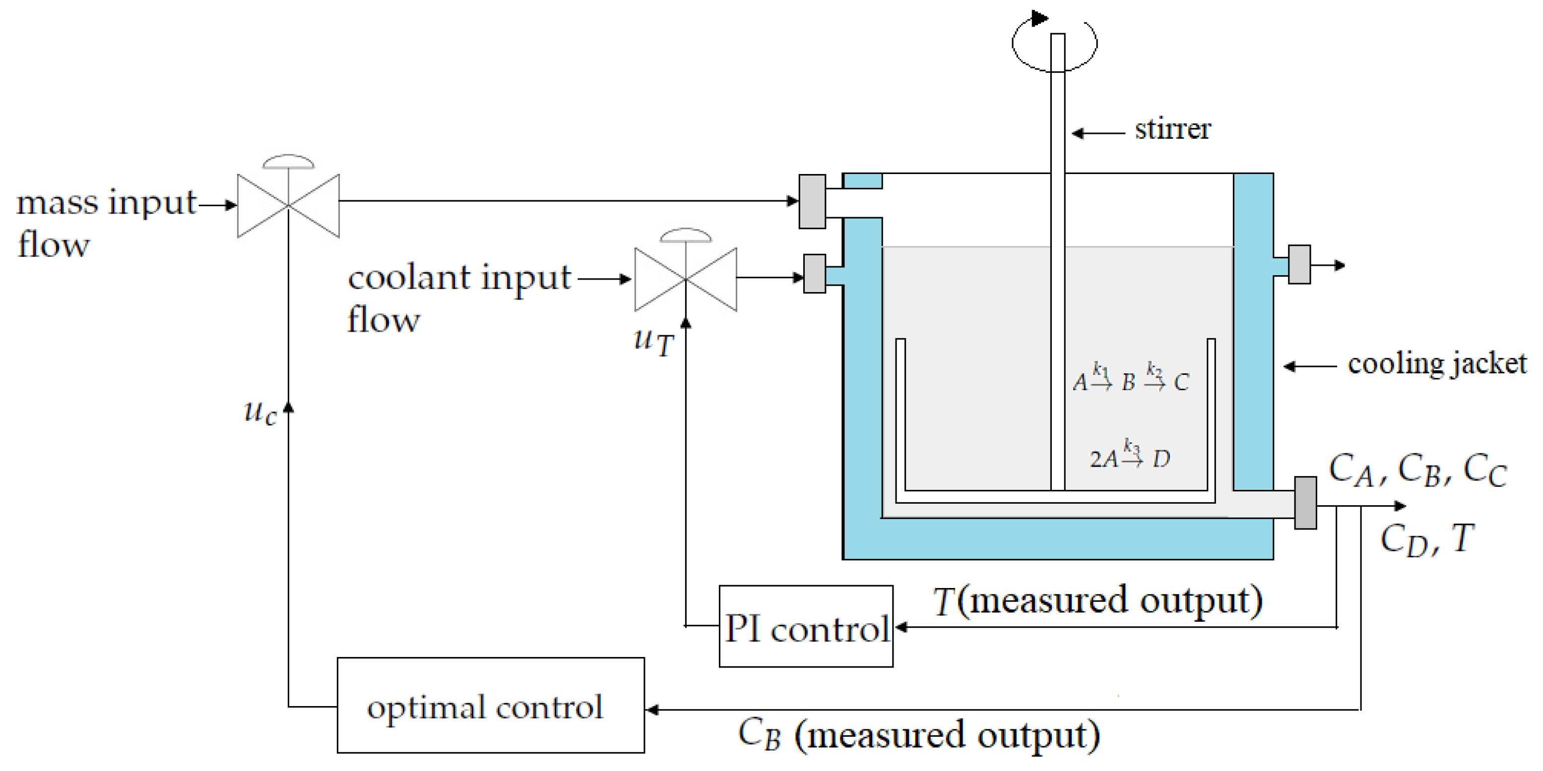
Upon initiation of the proposed closed-loop operation, the temperature of the reactor is regulated via the temperature of the cooling jacket, which is considered the manipulated variable , under a standard PI control structure. The controller gains are min and min, which are calculated by an identification process via a step disturbance in the temperature control input and the application of internal model control (IMC) tuning rules [51]. Figure 1 shows a generalized scheme of the closed-loop operation of an exothermic CSTR.
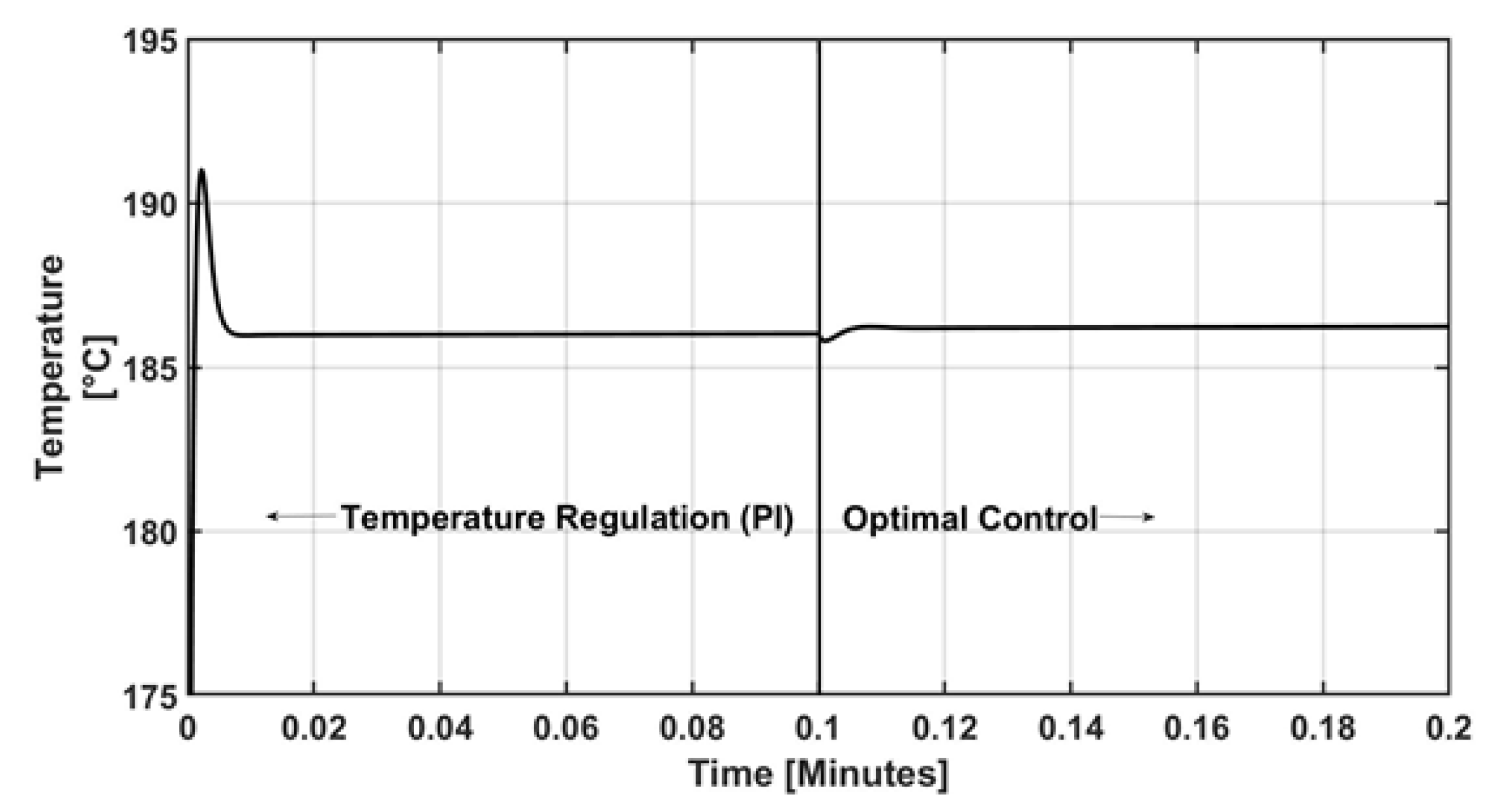
As can be observed in Figure 2, the temperature response of the closed-loop reactor is increasingly close to the required set point ( 185 °C), maintaining a small offset of 2.3 °C. Furthermore, when the reactor temperature is in the steady state (isothermal operation), at min, the optimal controller is activated. This is a significant disturbance in the thermal behavior of the reactor, but the temperature PI controller is able to resist it with an acceptable margin and maintains a temperature of 187 °C, again with a small offset of °C from the required set point. Thus, the PI controller is able to maintain the isothermal operation of the reactor, as illustrated in Figure 3, which shows that the temperature control input has a brief temperature decrease to 50 °C but, almost immediately, it behaves as a first order-type response and reaches a steady state of 97 °C. The temperature of the reactor is maintained within a small range around the required set point. When the optimal controller has been activated, an increase in the mass input flow is required to increase the concentration of chemical reactant A. Then, the temperature controller increases the temperature of the cooling jacket to 116 °C, initiating the chemical pathway that forms product B, which is the desired product. This reaction pathway has a high activation energy (see Table 1), so sufficient energy must be maintained to continue generating product B. In this sense, the temperature controller facilitates the supply of the necessary energy to generate product B.
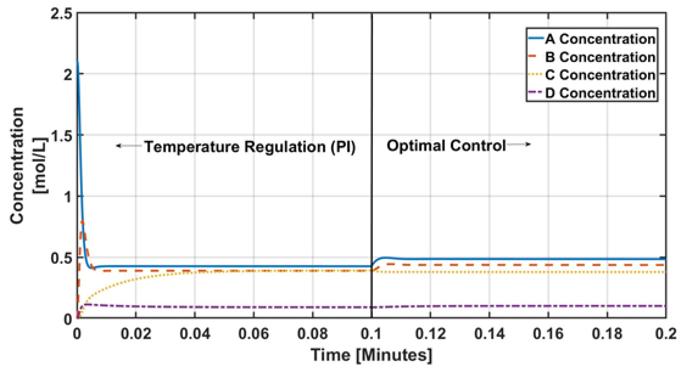
As previously mentioned, the objective is to optimize the productivity of the generation of chemical product B, which is an intermediate compound in the reaction network. Compound B is simultaneously a product and a reactant, so the optimal control must solve this chemical selectivity problem. As observed in Figure 4, after the operation is initiated, the concentration of the main reactant A is consumed from the initial condition via temperature effects (recall that compound A reacts in a parallel reaction). Then, the concentration of compound B increases due to temperature effects and reaches a steady-state value of mol/L, and when the optimal controller is activated, this concentration increases to mol/L. However, as can be seen below, the optimal controller increases the outlet mass flow and significantly increases the productivity. Furthermore, the dynamic behavior of the uncontrolled concentration is stable. Therefore, the results of numerical experiments show that the zero or inner dynamic of the reactor is stable and, as a consequence, the reactor is stabilizable.
Figure 5 shows the control effort of the optimal controller. The corresponding mass control input is adjusted to a nominal value ( mol/L) when the process is operating under the temperature regulation regimen. When the optimal controller is activated at min, the corresponding input flow drastically and rapidly increases to mol/L. This is an important characteristic of the behavior of the control input. Because of this substantial flow increase, the productivity of the reactor increases, as shown below (recall that the reactor productivity P is defined as ).
As mentioned previously, the optimal controller requires online information about the reaction rate term of chemical compound B. To provide this information, an observer-based uncertainty estimator (see Equation (41)) is coupled with the control algorithm. Figure 6 shows the performance of the proposed observer, where the observer gain is . The results of numerical experiments show that the controller has adequate performance, despite the significant disturbances related to the activation of the temperature and productivity controllers.
Finally, as one of the main results, Figure 7 shows the productivity performance of compound B in the reactor. When the reactor operates in the open-loop regimen, the steady-state productivity is reached at mol/L min, and when the proposed control strategy is applied, the productivity is increased to mol/L min in the first step of control temperature operation. When the optimal controller is activated, the corresponding productivity of compound B is successfully increased to mol/L min.
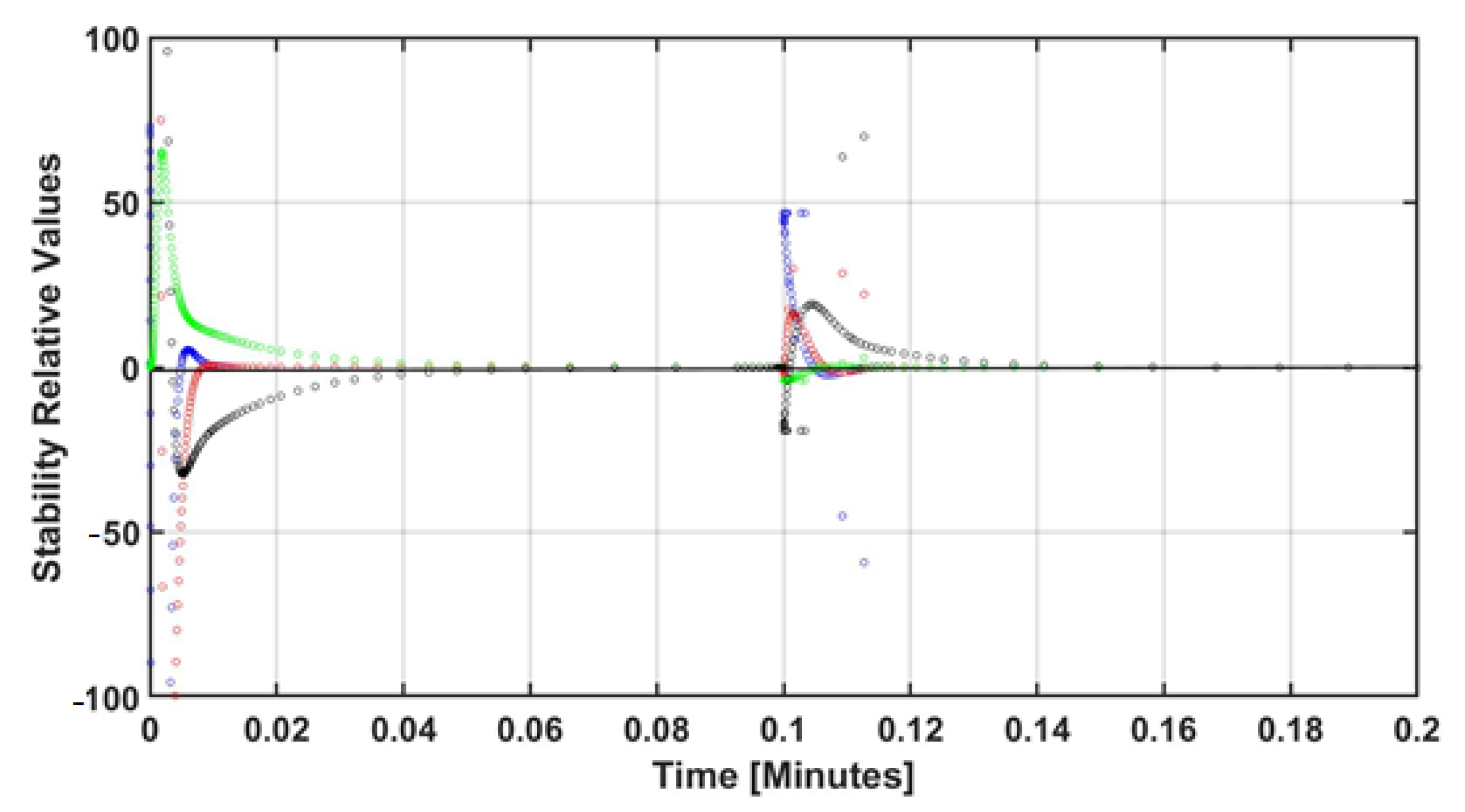
Figure 8 depicts the behavior of the relative stability values, i.e., the time derivatives of the uncontrolled concentrations, from the analysis of closed-loop stability in accordance with inequality (52). After the startup of the reactor under the temperature closed-loop regimen, compounds B and C are unstable because their relative values are positive, but their corresponding relative stability values asymptotically approach zero, becoming stable state variables. Compounds A and D show dynamic trajectories that are close to zero, indicating that they are acting as stable state variables. When the optimal controller is activated, the reactor dynamics undergo a considerable disturbance, and all relative stability values become positive, with the exception of compound D, whose relative value is always close to zero. As observed in the figure, all the zero dynamics of the reactor asymptotically reach a stable operating condition. These results agree with the dynamic behavior of the uncontrolled concentrations shown in Figure 4.
5. Conclusions
This work presents a two-input two-output (TITO) control strategy in which the control pairs are the reactor temperature/jacket temperature and productivity/input mass flow. At the first stage, the proposed closed-loop strategy aims to regulate the reactor temperature via a standard PI control law to increase the concentration of chemical compound B via a temperature increase until the reactor operation reaches isothermal conditions. Furthermore, an optimal controller designed by using the Euler–Lagrange approach is proposed. An important characteristic is that the Lagrangian is based on the model equation of the reactor, and when it is included in the corresponding functional, an analytic and explicit form of the corresponding controller can be obtained. This avoids the high computational effort required to numerically calculate the controller system, which is a common issue in other optimization strategies. The reactor productivity, which is the objective function, is optimized for compound B. The optimal controller design depends on online measurement of the reaction rate, which is unavailable. However, a reduced-order uncertainty observer is coupled with the controller to provide the required feedback term. The numerical results show the efficiency of the proposed TITO control methodology, and the temperature regulation regimen is confirmed to increase the productivity of the reactor by 40% in comparison with the open-loop operation. The increase in productivity after temperature regulation achieves optimal control is 32.15%, and the global productivity increase with the optimal control operation is 85.4% compared with the open-loop operation. To build on the theoretical results for the optimal controller design and the initial positive results of numerical experiments, future work will be oriented to real-time implementation to validate the performance of the proposed control strategy.
Author Contributions
Conceptualization, R.A.-L. and J.L.M.-M.; methodology, R.A.-L.; software, J.L.M.-M. and V.G.-C.; validation, R.A.-L., J.L.M.-M. and V.G.-C.; formal analysis, R.A.-L. and J.L.M.-M.; investigation, R.A.-L.; writing—original draft preparation, R.A.-L.; writing—review and editing, J.L.M.-M. and V.G.-C. All authors have read and agreed to the published version of the manuscript.
Funding
The APC was funded by the Comisión de Operación y Fomento de Actividades Académicas del Instituto Politécnico Nacional.
Institutional Review Board Statement
Not applicable.
Informed Consent Statement
Not applicable.
Data Availability Statement
Not applicable.
Conflicts of Interest
The authors declare no conflict of interest.
References
- Roberge, D.; Noti, C.; Irle, E.; Eyholzer, M.; Rittiner, B.; Penn, G.; Schenkel, B. Control of Hazardous Processes in Flow: Synthesis of 2-Nitroethanol. J. Flow Chem. 2014, 4, 26–34. [Google Scholar] [CrossRef] [Green Version]
- Chehade, G.; Dincer, I. Advanced Kinetic Modelling and Simulation of a New Small Modular Ammonia Converter. Chem. Eng. Sci. 2021, 236, 116512. [Google Scholar] [CrossRef]
- Contreras, L.A.; Franco, H.A.; Alvarez, J. Saturated output-feedback nonlinear control of a 3-continuous exothermic reactor train. IFAC-Pap. Online 2018, 51, 425–430. [Google Scholar] [CrossRef]
- Gavalas, G.R. Uniform Systems with Chemical Change. In Nonlinear Differential Equations of Chemically Reacting Systems; Springer Tracts in Natural Philosophy; Springer: Berlin/Heidelberg, Germany, 1968; Volume 17. [Google Scholar]
- Ackermann, J.; Kaesbauer, D. Design of robust PID controllers. In Proceedings of the European Control Conference (ECC), Porto, Portugal, 4–7 September 2001; pp. 522–527. [Google Scholar]
- Aguilar, R.; Poznyak, A.; Martínez-Guerra, R.; Maya-Yescas, R. Temperature control in catalytic cracking reactors via a robust PID controller. J. Process Control 2002, 12, 695–705. [Google Scholar] [CrossRef]
- Oriolo, G.; De Luca, A.; Vendittelli, M. WMR control via dynamic feedback linearization: Design, implementation, and experimental validation. IEEE Trans. Control Syst. Technol. 2002, 10, 835–852. [Google Scholar] [CrossRef]
- Barkhordari, M.; Jahed-Motlagh, M.R. Stabilization of a CSTR with two arbitrarily switching modes using modal state feedback linearization. Chem. Eng. J. 2009, 155, 838–843. [Google Scholar] [CrossRef]
- Rubio, J.J. Robust feedback linearization for nonlinear processes control. ISA Trans. 2018, 74, 155–164. [Google Scholar] [CrossRef]
- Zhang, Z.; Wu, Z.; Durand, H.; Albalawi, F.; Christofides, P.D. On integration of feedback control and safety systems: Analyzing two chemical process applications. Chem. Eng. Res. Des. 2018, 132, 616–626. [Google Scholar] [CrossRef] [Green Version]
- Kravaris, C.; Kantor, J.C. Geometric methods for nonlinear process control. 2. Controller synthesis. Ind. Eng. Chem. Res. 1990, 29, 2310–2323. [Google Scholar] [CrossRef]
- Alvarez-Gallegos, J. Nonlinear regulation of a Lorenz system by feedback linearization techniques. Dyn. Control 1994, 4, 277–298. [Google Scholar] [CrossRef]
- Jana, A.K. Nonlinear State Estimation and Generic Model Control of a Continuous Stirred Tank Reactor. Int. J. Chem. React. Eng. 2007, 5, A42. [Google Scholar] [CrossRef]
- Cott, B.J.; Macchietto, S. Temperature control of exothermic batch reactors using generic model control. Ind. Eng. Chem. Res. 1989, 28, 1177–1184. [Google Scholar] [CrossRef]
- Chu, Y.; You, F. Model-based integration of control and operations: Overview, challenges, advances, and opportunities. Comput. Chem. Eng. 2015, 83, 2–20. [Google Scholar] [CrossRef]
- Baruah, S.; Dewan, L. A comparative study of PID based temperature control of CSTR using Genetic Algorithm and Particle Swarm Optimization. In Proceedings of the International Conference on Emerging Trends in Computing and Communication Technologies (ICETCCT), Dehradun, India, 17–18 November 2017; pp. 1–6. [Google Scholar]
- Khanduja, N.; Bhushan, B. CSTR Control Using IMC-PID, PSO-PID, and Hybrid BBO-FF-PID Controller. In Applications of Artificial Intelligence Techniques in Engineering; Malik, H., Srivastava, S., Sood, Y., Ahmad, A., Eds.; Advances in Intelligent Systems and Computing; Springer: Singapore, 2019; Volume 697. [Google Scholar]
- Romero-Bustamante, J.A.; Moguel-Castañeda, J.G.; Puebla, H.; Hernandez-Martinez, E. Robust Cascade Control for Chemical Reactors: An Approach based on Modelling Error Compensation. Int. J. Chem. React. Eng. 2017, 15. [Google Scholar] [CrossRef]
- Murugesan, R.; Solaimalai, J.; Chandran, K. Computer-Aided Controller Design for a Nonlinear Process Using a Lagrangian-Based State Transition Algorithm. Circuits Syst. Signal Process 2020, 39, 977–996. [Google Scholar] [CrossRef]
- Zerari, N.; Chemachema, M. Robust adaptive neural network prescribed performance control for uncertain CSTR system with input nonlinearities and external disturbance. Neural Comput. Applic. 2020, 32, 10541–10554. [Google Scholar] [CrossRef]
- Zhang, R.; Wu, S.; Cao, Z.; Lu, J.; Gao, F. A Systematic Min–Max Optimization Design of Constrained Model Predictive Tracking Control for Industrial Processes against Uncertainty. IEEE Trans. Control Syst. Technol. 2018, 26, 2157–2164. [Google Scholar] [CrossRef]
- Maurer, J.; Freund, H. Efficient calculation of constraint back-offs for optimization under uncertainty: A case study on maleic anhydride synthesis. Chem. Eng. Sci. 2018, 192, 306–317. [Google Scholar]
- Rodríguez-Pérez, B.E.; Flores-Tlacuahuac, A.; Ricardez-Sandoval, L.; Lozano, F.J. Optimal Water Quality Control of Sequencing Batch Reactors Under Uncertainty. Ind. Eng. Chem. Res. 2018, 57, 9571–9590. [Google Scholar] [CrossRef]
- Jia, R.; You, F. Multi-stage economic model predictive control for a gold cyanidation leaching process under uncertainty. AIChE J. 2021, 67, e17043. [Google Scholar] [CrossRef]
- Aguilar, R.; Martínez-Guerra, R.; Poznyak, A. Reaction heat estimation in continuous chemical reactors using high gain observers. Chem. Eng. J. 2002, 87, 351–356. [Google Scholar] [CrossRef]
- Aguilar-López, R. State estimation for nonlinear systems under model unobservable uncertainties: Application to continuous reactor. Chem. Eng. J. 2005, 108, 139–144. [Google Scholar] [CrossRef]
- Harinath, E.; Foguth, L.C.; Paulson, J.A.; Braatz, R.D. Nonlinear model predictive control using polynomial optimization methods. In Proceedings of the IEEE American Control Conference (ACC), Boston, MA, USA, 6–8 July 2016; pp. 1–6. [Google Scholar]
- Hashem, I.; Telen, D.; Nimmegeers, P.; Logist, F.; Van Impe, J. A novel algorithm for fast representation of a Pareto front with adaptive resolution: Application to multi-objective optimization of a chemical reactor. Comput. Chem. Eng. 2017, 106, 544–558. [Google Scholar] [CrossRef]
- Puschke, J.; Djelassi, H.; Kleinekorte, J.; Hannemann-Tamás, R.; Mitsos, A. Robust dynamic optimization of batch processes under parametric uncertainty: Utilizing approaches from semi-infinite programs. Comput. Chem. Eng. 2018, 116, 253–267. [Google Scholar] [CrossRef]
- Maurer, J.; Freund, H. Optimization under uncertainty in chemical engineering: Comparative evaluation of unscented transformation methods and cubature rules. Chem. Eng. Sci. 2018, 183, 329–345. [Google Scholar]
- Bernardo, F.P.; Pistikopoulos, E.N.; Saraiva, P.M. Integration and computational issues in stochastic design and planning optimization problems. Ind. Eng. Chem. Res. 1999, 38, 3056–3068. [Google Scholar] [CrossRef]
- Bernardo, F.P.; Pistikopoulos, E.N.; Saraiva, P.M. Quality costs and robustness criteria in chemical process design optimization. Comput. Chem. Eng. 2001, 25, 27–40. [Google Scholar] [CrossRef] [Green Version]
- Zhang, C.; Seow, V.Y.; Chen, X.; Too, H.P. Multidimensional heuristic process for high-yield production of astaxanthin and fragrance molecules in Escherichia coli. Nat. Commun. 2018, 9, 1–12. [Google Scholar] [CrossRef] [Green Version]
- Yuan, J.; Liu, C.; Zhang, X.; Xie, J.; Feng, E.; Yin, H.; Xiu, Z. Optimal control of a batch fermentation process with nonlinear time-delay and free terminal time and cost sensitivity constraint. J. Process Control 2016, 44, 41–52. [Google Scholar] [CrossRef] [Green Version]
- Gurubel, K.J.; Osuna-Enciso, V.; Coronado-Mendoza, A.; Cuevas, E. Optimal control strategy based on neural model of nonlinear systems and evolutionary algorithms for renewable energy production as applied to biofuel generation. J. Renew. Sustain. Energy 2017, 9, 033101. [Google Scholar] [CrossRef]
- Goud, H.; Swarnkar, P. Investigations on Metaheuristic Algorithm for Designing Adaptive PID Controller for Continuous Stirred Tank Reactor. MAPAN 2019, 34, 113–119. [Google Scholar] [CrossRef]
- Zhang, Y.; Li, S.; Liao, L. Near-optimal control of nonlinear dynamical systems: A brief survey. Annu. Rev. Control 2019, 47, 71–80. [Google Scholar] [CrossRef]
- Bailo, R.; Bongini, M.; Carrillo, J.A.; Kalise, D. Optimal consensus control of the Cucker-Smale model. IFAC-Pap. OnLine 2018, 51, 1–6. [Google Scholar] [CrossRef]
- Lara-Cisneros, G.; Aguilar-López, R.; Femat, R. On the dynamic optimization of methane production in anaerobic digestion via extremum-seeking control approach. Comput. Chem. Eng. 2015, 75, 49–59. [Google Scholar] [CrossRef]
- Verleysen, K.; Coppitters, D.; Parente, A.; De Paepe, W.; Contino, F. How can power-to-ammonia be robust? Optimization of an ammonia synthesis plant powered by a wind turbine considering operational uncertainties. Fuel 2020, 266, 117049. [Google Scholar] [CrossRef]
- Alvarez-Ramirez, J.; Puebla, H. On classical PI control of chemical reactors. Chem. Eng. Sci. 2001, 56, 2111–2121. [Google Scholar] [CrossRef]
- Amte, V.; Nistala, S.; Malik, R.; Mahajani, S. Attainable regions of reactive distillation—Part III. Complex reaction scheme: Van de Vusse reaction. Chem. Eng. Sci. 2011, 66, 2285–2297. [Google Scholar] [CrossRef]
- Van de Vusse, J.G. Plug-flow type reactor versus tank reactor. Chem. Eng. Sci. 1964, 19, 994–997. [Google Scholar] [CrossRef]
- Trierweiler, J.O. A Systematic Approach to Control Structure Design. Ph.D. Thesis, Universität Dortmund, Dortmund, Germany, 1997. [Google Scholar]
- Rubi, V.A.; Deo, A.; Kumar, N. Temperature control of CSTR using PID Controller. Int. J. Eng. Comput. Sci. 2015, 4, 11902–11905. [Google Scholar]
- Kumar, M.; Prasad, D.; Giri, B.S.; Singh, R.S. Temperature control of fermentation bioreactor for ethanol production using IMC-PID controller. Biotechnol. Rep. 2019, 22, e00319. [Google Scholar] [CrossRef]
- Aguilar-López, R. Chaos Suppression via Euler-Lagrange Control Design for a Class of Chemical Reacting System. Math. Probl. Eng. 2018, 3802801. [Google Scholar] [CrossRef]
- Flores-Flores, J.P.; Martínez-Guerra, R. PI observer design for a class of nondifferentially flat systems. Int. J. Appl. Math. Comput. Sci. 2019, 29, 655–665. [Google Scholar] [CrossRef] [Green Version]
- Martínez-Guerra, R.; Cruz-Victoria, J.C.; Gonzalez-Galan, R.; Aguilar-Lopez, R. A new reduced-order observer design for the synchronization of Lorenz systems. Chaos Solitons Fractals 2006, 28, 511–517. [Google Scholar] [CrossRef]
- Aguilar-Lopez, R.; Maya-Yescas, R. Inverse dynamics: A problem on transient controllability for industrial plants. Inverse Probl. Sci. Eng. 2008, 16, 811–827. [Google Scholar] [CrossRef]
- Babatunde, A.O.; Ray, W.H. Process Dynamics Modeling Control; Oxford University Press: Oxford, UK, 1994. [Google Scholar]
Figure 1.
Exothermic CSTR.

Figure 2.
Closed-loop dynamic behavior of the reactor temperature.

Figure 3.
Control effort for temperature regulation.
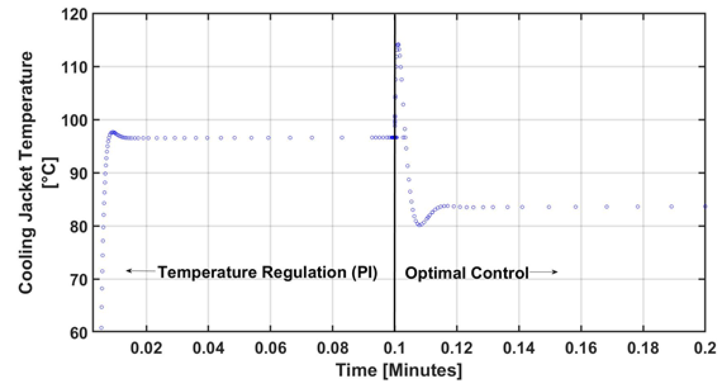
Figure 4.
Closed-loop dynamic behavior of concentrations.

Figure 5.
Control effort of the optimal controller.
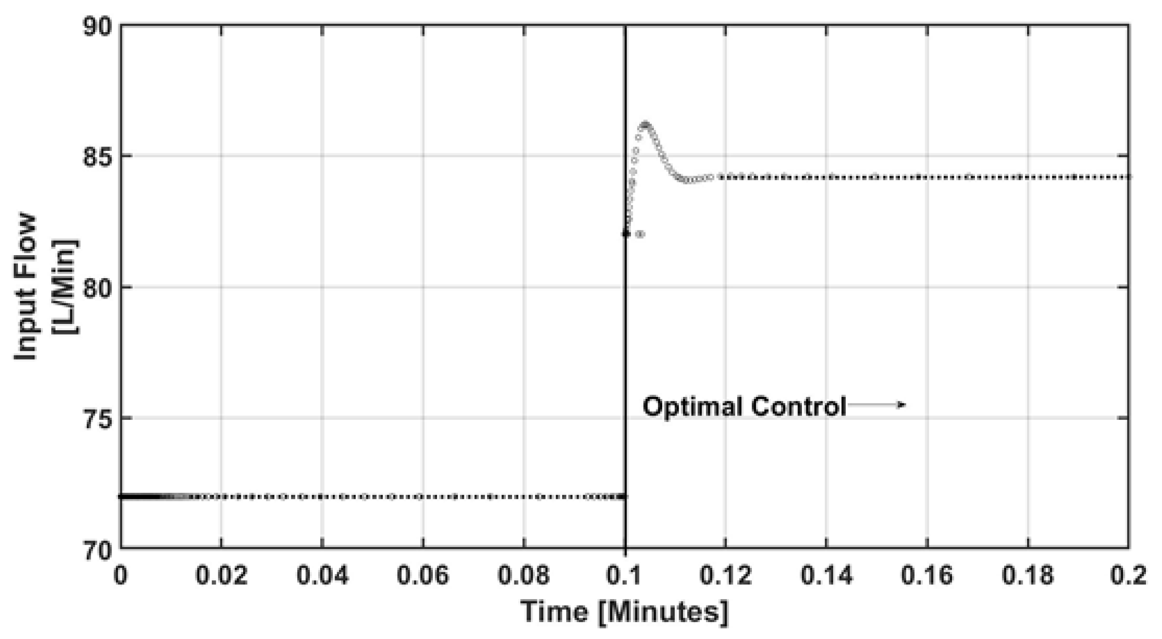
Figure 6.
Dynamic performance of the uncertainty estimator.
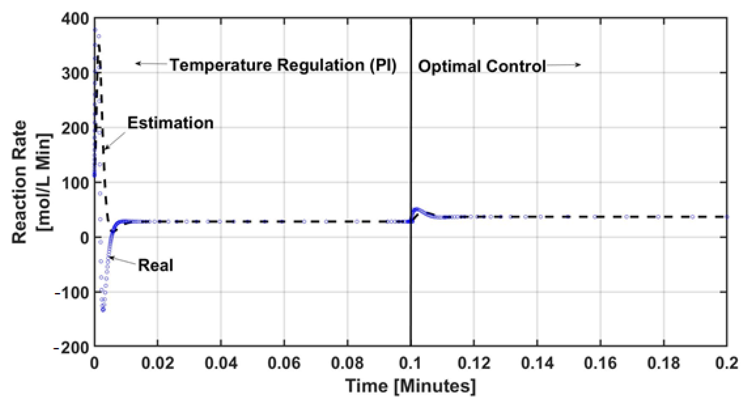
Figure 7.
Open-loop and closed-loop dynamic behaviors of reactor productivity for compound B.
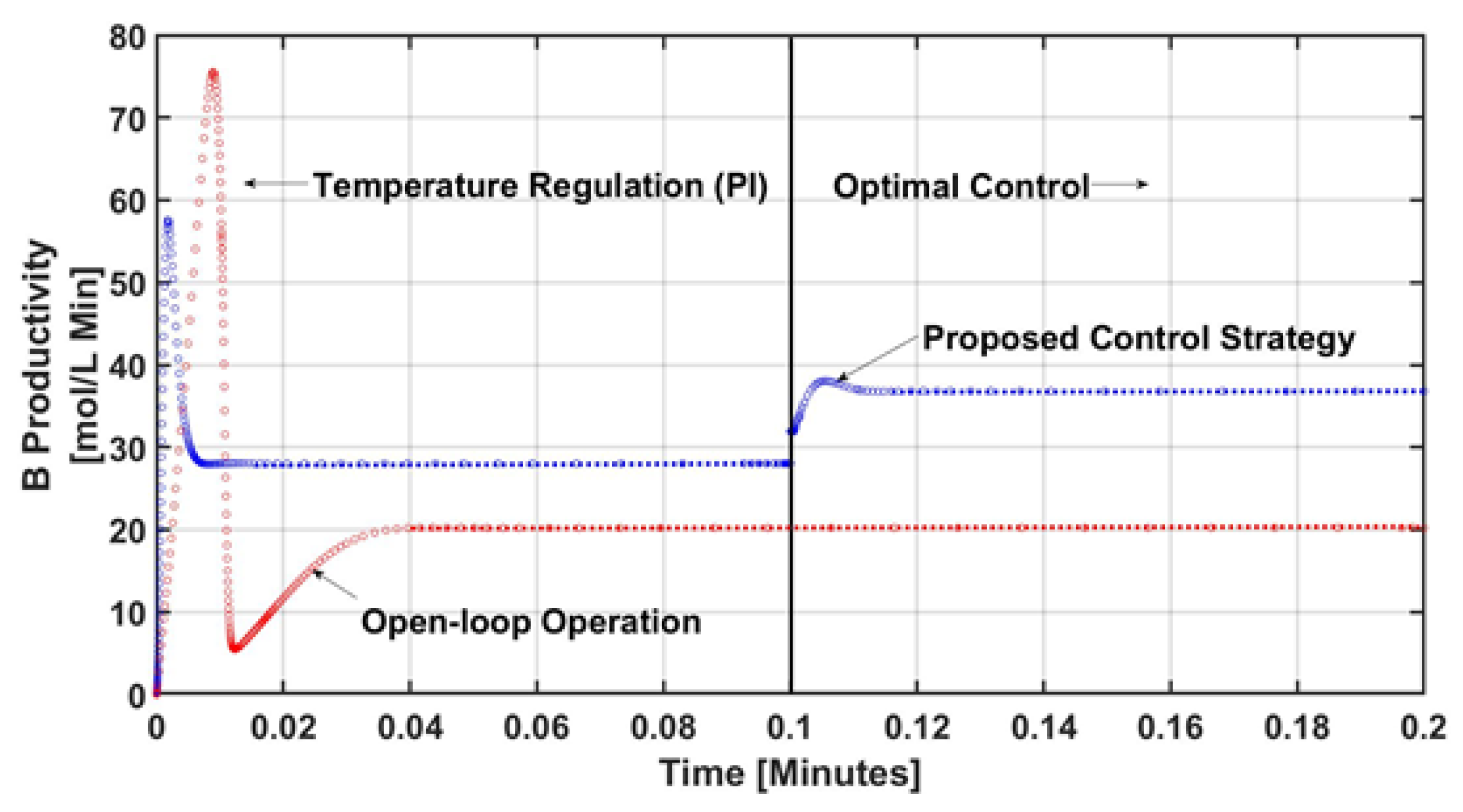
Figure 8.
Relative stability values for uncontrolled concentrations (red—compound A; blue—compound B; green—compound C; black—compound D).
Figure 8.
Relative stability values for uncontrolled concentrations (red—compound A; blue—compound B; green—compound C; black—compound D).


Table 1.
Reactor parameters.
| Description | Parameter | Value | Units |
|---|---|---|---|
| Heat transfer area | A | 0.215 | m |
| Temperature initial condition | 387.05 | K | |
| Heat transfer coefficient | U | 67.2 | kJ·minmK |
| Heat capacity | kJ·kg K | ||
| Nominal cooling jacket temperature | 125 | C | |
| Reacting mixture density | 934.2 | kg·m | |
| Reactor volume | V | 0.01 | m |
| Concentration initial conditions | |||
| Pre-exponential kinetic factors | |||
| Activation energies | |||
| Reaction heat |
Publisher’s Note: MDPI stays neutral with regard to jurisdictional claims in published maps and institutional affiliations. |
© 2021 by the authors. Licensee MDPI, Basel, Switzerland. This article is an open access article distributed under the terms and conditions of the Creative Commons Attribution (CC BY) license (https://creativecommons.org/licenses/by/4.0/).
Share and Cite
MDPI and ACS Style
Aguilar-López, R.; Mata-Machuca, J.L.; Godinez-Cantillo, V. A TITO Control Strategy to Increase Productivity in Uncertain Exothermic Continuous Chemical Reactors. Processes 2021, 9, 873. https://doi.org/10.3390/pr9050873
AMA Style
Aguilar-López R, Mata-Machuca JL, Godinez-Cantillo V. A TITO Control Strategy to Increase Productivity in Uncertain Exothermic Continuous Chemical Reactors. Processes. 2021; 9(5):873. https://doi.org/10.3390/pr9050873
Chicago/Turabian StyleAguilar-López, Ricardo, Juan Luis Mata-Machuca, and Valeria Godinez-Cantillo. 2021. "A TITO Control Strategy to Increase Productivity in Uncertain Exothermic Continuous Chemical Reactors" Processes 9, no. 5: 873. https://doi.org/10.3390/pr9050873
Note that from the first issue of 2016, this journal uses article numbers instead of page numbers. See further details here.