Determination of a Bubble Drag Coefficient during the Formation of Single Gas Bubble in Upward Coflowing Liquid


Faculty of Chemical Engineering and Technology, Cracow University of Technology, ul. Warszawska 24, 31-155 Kraków, Poland
*
Authors to whom correspondence should be addressed.
Processes 2020, 8(8), 999; https://doi.org/10.3390/pr8080999
Submission received: 26 July 2020
/
Revised: 11 August 2020
/
Accepted: 12 August 2020
/
Published: 17 August 2020
(This article belongs to the Section Chemical Processes and Systems)
Abstract
:Bubble flow is present in many processes that are the subject of chemical engineering research. Many correlations for determination of the equivalent bubble diameter can be found in the scientific literature. However, there are only few describing the formation of gas bubbles in flowing liquid. Such a phenomenon occurs for instance in airlift apparatuses. Liquid flowing around the gas bubble creates a hydraulic drag force that leads to reduction of the formed bubble diameter. Usually the value of the hydraulic drag coefficient, , for bubble formation in the flowing liquid is assumed to be equal to the drag coefficient for bubbles rising in the stagnant liquid, which is far from the reality. Therefore, in this study, to determine the value of the drag coefficient of bubbles forming in flowing liquid, the diameter of the bubbles formed at different liquid velocity was measured using the shadowgraphy method. Using the balance of forces affecting the bubble formed in the coflowing liquid, the hydraulic drag coefficient was determined. The obtained values of the drag coefficient differed significantly from those calculated using the correlation for gas bubble rising in stagnant liquid. The proposed correlation allowed the determination of the diameter of the gas bubble with satisfactory accuracy.
1. Introduction
Multiphase flows are omnipresent in the chemical engineering processes [1]. One example of the multiphase flow is the flow of gas through a liquid layer. When the gas flow rate is high enough so that a large number of gas bubbles simultaneously flows through the liquid, such a process is known as bubbling. The use of this phenomenon is crucial in many fields, including chemical and process engineering, bioprocess engineering, environmental engineering, and wastewater treatment. A classic example of the bubbling application can be seen in microbiological sewage treatment [2,3,4]. Typical apparatuses employing the phenomenon of bubbling are bubble column [5] and airlift apparatus [6]. More sophisticated systems from the design point of view in which the bubble flow occurs are hybrid airlift apparatuses [7,8].
Despite decades of research, a large number of new scientific papers is published each year regarding the flow of gas bubbles through liquid layer. Kulkarni and Joshi [9] made a comprehensive review of the available models of bubble formation, bubble rise, and drag coefficient. Prediction of the hydrodynamic properties of the gas bubbles, as well as determination of the characteristics of their detachment from the orifice are key in the design of apparatuses and processes of heat and mass transfer in bubble flows. Knowing the size of the liquid–gas interface area is crucial, as its increase leads to the intensification of the mass and heat transfer phenomena. The process of bubble formation and detachment is a complex problem, due to the large number of forces acting in the system (i.e., gravity, buoyancy, surface tension, drag, momentum flux of the gas phase, added mass inertial forces, or influence of the wake of previous bubble) and a large number of parameters determining these phenomena (e.g., physical properties or process parameters) [10].
Due to the benefits of the development of a liquid–gas interface, the flow of single bubbles through a liquid layer is rare in industry. Nevertheless, knowledge of the hydrodynamic properties and parameters of single bubbles is also essential, because many mathematical models describing bubbling contain expressions concerning the flow of single bubbles.
The flow of the gas phase through a stagnant liquid is a phenomenon relatively well-known and comprehensively described in the literature. Parameters such as bubble diameter [11,12], drag coefficient [13,14], or rise velocity [15,16] were the subject of many publications in the last decades. Despite the lack of universal correlations, hydrodynamics of bubbles formed in stationary liquid is considered a relatively well-known issue.
For a stagnant liquid layer and infinitely small volumetric flow rate of the gas phase, bubble diameter can be calculated using simple force balance approach. In these conditions, three main forces act on a bubble—buoyancy, gravity, and surface tension. The gravity and surface tension forces are pointed downwards, so they prevent the bubble detachment. The buoyancy force is pointed upward, because gas density is lower than the liquid density. At the moment of detachment of a gas bubble, the three forces are in balance, which could be written as:
where,
- —bubble diameter, m
- —gravitational acceleration, m/s2
- —liquid density, kg/m3
- —gas density, kg/m3
- —inner nozzle diameter, m
- —liquid surface tension, N/m
The terms on the left-hand side of Equation (1) represent buoyancy and gravity forces, respectively, whereas the term on the right-hand side represents surface tension force. By rearranging the equation, bubble diameter could be calculated:
It can be observed, that lowering the nozzle diameter, , or surface tension (e.g., by adding surfactants), , results in a decrease of the bubble size. Equation (2) can be used to calculate bubble diameter only for small volumetric gas flow rates. Surface tension then plays an important role in the formation of gas bubbles. As the gas flow increases, the momentum flux of the gas phase and the added mass inertial force increase.
Volumetric gas flow rate can be expressed as a product of bubble volume and bubble detachment frequency, that is:
where,
- —gas volumetric flow rate, m3/s
- —bubble detachment frequency, Hz
Usually, the volumetric flow rate is a known process variable and detachment frequency need to be calculated. Rearranging the above equation, bubble detachment frequency could be obtained using the following formula:
On the other hand, description of the gas phase flow in the flowing liquid is poorly examined. As already mentioned, concurrent flow of a liquid phase and gas bubbles occurs among others in airlift apparatuses. According to the experimental results presented in the literature, bubble size distribution is strongly dependent on the liquid flow velocity [17,18,19]. Chuang and Goldschmidt [20] proposed a simple model based on a force balance approach. The model proposed by the authors could be expressed as:
where,
- —drag coefficient, -
- —area of influence of drag force, m2
- —liquid velocity, m/s
- —displacement of the center of mass of the bubble, m
- —time, s
- —mass, kg
In Equation (5), the terms on the left side of the equation, respectively, represent the buoyancy force of the gas bubble, and the drag force referred to the velocity, relative to the center of the formed bubble. The terms on the right represent surface tension force and the added mass inertial force, respectively. The value of the hydraulic drag coefficient was calculated using the following equation:
where:
—Reynolds number, -
The above correlation is valid in the range of Reynolds number . In the definition of the Reynolds number Chuang and Goldschmidt [20] referred to the liquid velocity relative to the center of the bubble with the bubble diameter used as the characteristic length:
where:
—liquid dynamic viscosity coefficient, Pa·s
The distance from the center of the bubble to the orifice tip, , can be calculated using the Pythagorean theorem, as:
Thus, the rising velocity of the center of mass of the formed bubble attached to orifice, , at the moment of its detachment, could be calculated using the following equation:
from the definition of volumetric flow rate we obtain:
where,
- —gas volumetric flow rate, m3/s
- —volume, m3
Combining Equation (10) with Equation (3) yields:
considering that , Equation (9) could be simplified into:
the displaced mass, , could be calculated as:
whereas the last term in Equation (5), i.e., the added mass inertial force could be calculated as:
The influence of the gas bubble weight and the gas phase momentum flux was omitted in the above model because their contribution was several orders of magnitude smaller than the contribution of the other terms of the model. In study [20], authors examined nozzles with a relatively small internal diameter, which was 13.6 and 48.1 μm. The liquid velocity varied in the range of 0–2.7 m/s and the bubbles were formed at a frequency of 10 Hz and 170 Hz. The formed bubble diameters ranged between 50–1200 μm.
A similar approach was used by Terasaka et al. [21]; in comparison to the model developed by Chuang and Goldschmidt [20], their model was supplemented with bubble weight and gas phase momentum flux, which yielded the following expression:
The authors examined in their work the influence of such parameters like liquid velocity (0–0.173 m/s), nozzle inner diameter (1.19–3.00 mm), gas phase volumetric flow rate (0.13 10−6–5.11 10−6 m3/s), and gas chamber volume (33.3 10−6–89.9 10−6 m3). The nozzle outer diameter, , was about 4 mm and analyzed bubble diameter, , ranged between 3.5–12 mm.
Sada et al. [22] proposed a model connecting the bubble diameter with the modified Froude number. In their study, the authors presented a model that took into account the buoyancy force and the drag force of the bubble detaching from the orifice. It was assumed that the value of the drag coefficient, , was equal to 0.44, which corresponded to the drag coefficient of the turbulent sedimentation of spherical particles in fluids. Based on such assumptions, the authors used the concept of a modified Froude number relative to the diameter of the bubble and accounted for the liquid velocity. The modified Froude number could be expressed as:
where,
- —modified Froude number (Sada et al. [22]), -
- —gas velocity, m/s
- —superficial liquid velocity, m/s
According to [22], the diameter of the bubble could be determined, depending on the adopted flow range, from equations in the following form:
where,
, —experimental coefficients,
In their work, Sada et al. [22] examined the influence of volumetric gas flow rate (0.33 10−6–36.2 10−6 m3/s) and superficial liquid flow velocity (0–1.549 m/s). The authors used two different gas orifices of 0.86/1.30 mm and 3.05/4.00 mm (). The generated bubble diameter, , ranged between 3–12 mm.
Muilwijk and Van den Akker [23] studied the formation of gas bubbles in Newtonian liquids, both in stagnant and flowing states, concurrent with the gas phase liquids. They correlated the diameters of gas bubbles with the dimensionless Bond, , and Froude, , numbers. Based on the conducted experimental research, the authors proposed the following formula for the calculation of the diameter of gas bubble in a stagnant liquid, detached from the nozzle:
where,
- —Bond number,
- —Froude number,
The correlation regarding the diameter of gas bubbles forming in the coflowing liquid is an extension of the formula referring to the stagnant liquid, Equation (18), and is expressed as:
where Bond and Froude numbers are defined as:
In their study, Muilwijk and Van den Akker [23] examined the influence of nozzle internal diameter (0.79–2.06 mm), nozzle external diameter (1.59 mm or 3.18 mm), volumetric gas flow rate (0.5 10−6–4.5 10−6 m3/s), and liquid velocity (0–0.4 m/s), on bubble formation rates (10–55 Hz) and bubble sizes (3.4–6.7 mm).
It could be observed that two different approaches were used in the literature to determine the diameter of bubbles forming in a flowing liquid. One of them was based on dimensionless numbers (Sada et al. [22], Muilwijk, and Van den Akker [23]). By using classical or modified definitions of a selected dimensionless number (i.e., , , ), the authors tried to correlate their values with the diameter of the bubbles. Such correlations were derived from a certain specific range of experimental data, therefore, outside this range the correlations could be characterized by significant discrepancies between the calculated and experimental results.
Another way is to use a balance of forces acting on the bubble when it is detached from the nozzle (as in Chuang and Goldschmidt [20] or Terasaka et al. [21]). In theory, a given model is valid as long as the ranges of applicability of the appropriate terms are met, so such a model can be used even outside the range of the parameter values used during experiments. An additional advantage of models based on the balance of forces is the fact, that based on the apparatus operating conditions, such models can be easily simplified. If the contribution of some term is smaller by several orders of magnitude than the contribution of other terms, then it can be neglected without introducing a significant error in the results. This often leads to a major simplification of the employed model.
However, some inconsistency can be found in the models based on the force balance approach. One such inconsistency is the usage of the inappropriate correlation for calculating the value of the drag coefficient . The authors use correlations derived for the rise of bubbles in the stagnant liquid quite often. In such conditions, the velocity of the rising bubbles is closely correlated with their diameter. The drag coefficient is, therefore, actually only a function of the diameter of the flowing bubble. During the formation of gas bubbles in the flowing liquid, the relative velocity of the liquid can be arbitrarily changed. This might suggest that correlations for bubble flow in a stationary liquid might give erroneous results when describing bubble formation in a flowing liquid.
Various authors also disagree as to the surface that should be used in the term describing the impact of the bubble drag force. Chuang and Goldschmidt [20], in the original version of their model, suggest that the drag force should refer to the cross-sectional area of the bubble, i.e., . However, in the further part of their study they suggest that since the liquid flowing near the gas bubble that is formed must bypass the nozzle, the drag force acts only on the surface of the ring, limited from the outside by the diameter of the bubble, , and from the inside by the outer diameter of the nozzle, , which results in the surface equal to . Terasaka et al. [21] suggests, however, that the surface should refer to the horizontal diameter of the bubble, , therefore, it should be calculated as .
Similar inconsistences also concern the definition of Reynolds number. Chuang and Goldschmidt [20] use the bubble diameter, , as the characteristic length. However, since the liquid must bypass the nozzle, it seems more accurate to adopt an equivalent diameter for the annular surface, i.e., . On the other hand, under the conditions of bubble detachment, the bubble is connected with the inner edge of the nozzle, so in this case it seems more reasonable to use an equivalent diameter for the annulus, limited by the diameter of the bubble, , and by the internal diameter of the nozzle, , which gives an equivalent diameter of .
In addition, very often, the effect of the nozzle wall thickness is not explicitly specified. For instance, Chuang and Goldschmidt [20] did not specify the value of the outer diameter of the nozzles used, while Terasaka et al. [21] used nozzles with different internal diameters, but similar outer diameter ( mm).
The objective of this study was, therefore, to clarify discrepancies found in the literature related to gas bubble formation in the flowing Newtonian liquid. The main aims included determination of the value of the drag coefficient during the formation of bubbles in the concurrently flowing liquid, analysis of the impact of the gas distributor wall thickness, and identification of characteristic dimensions that should be used when determining the drag force.
2. Materials and Methods
2.1. Materials
In this work, air was used as the gas phase and tap water as the liquid phase. The average water temperature was 10 °C. The nozzle through which the air was injected was immersed in the liquid and had a length of about 0.15 m. During the flow through the nozzle, the air temperature decreased, therefore, it was assumed in the calculations that the air temperature was an average between the ambient temperature (20 °C) and the water temperature, i.e., 15 °C. The physical properties of the media that were used in the calculations are presented in Table 1. During the experiments, water temperature deviated no more than ±1 °C. In such a narrow temperature interval, liquid density and surface tension should not deviate more than ±1% and water viscosity should deviate no more than ±3%. On the other hand, air temperature did not deviate more than ±5 °C, which resulted in ±3% deviation in air density value.
2.2. Experimental Setup
A schematic drawing of the test stand is shown in Figure 1. The main part (denoted with number 1 in Figure 1) consisted of a square channel made of poly (methyl methacrylate), with a side length of 0.08 m. The water flow rate was controlled using a valve (2 in Figure 1) and its value was measured using a rotameter (3 in Figure 1). Water from the water supply network was introduced at the bottom of the column (4 in Figure 1). First, water flowed through two layers of packing consisting of Raschig rings, with a diameter of 5 mm and 16 mm, respectively (5 in Figure 1), to flatten the liquid velocity profile. Then, it flowed through two layers of flow straighteners (6 in Figure 1) to laminarize the liquid velocity profile. The third flow straightener was mounted near the column outlet to minimize the stream contraction. The air was supplied using an air compressor (7 in Figure 1) and its flow rate was controlled using a valve (8 in Figure 1). The nozzle (9 in Figure 1) was mounted at a distance of about 0.1 m from the second flow straightener. In the upper part of the column, there was a liquid and a gas phase outlet (10 in Figure 1). The images of flowing bubbles were recorded using a CMOS camera, allowing for high-speed image recording (11 in Figure 1). For better illumination of the bubbles, LED lighting was mounted on the opposite side of the column (12 in Figure 1).
Nine nozzles differing in internal and external diameters were used in this study. The internal diameter varied in the range of 0.8–2.1 mm. The wall thickness of the tubes was 0.1 mm or 0.45 mm. The nozzles were made of brass pipes bent at an angle of 90°. The length of the straight part of the nozzle was at least 20x the nozzle inner diameter, . The nozzle outlet was finished using precision files and fine sandpaper. The internal and external diameters of the nozzles used are reported in Table 2.
CMOS IDS UI-3130CP-C-HQ Rev.2 camera [24] was used to record the formation and flow of gas bubbles. The camera allowed to record images with a maximum frequency of 396 fps, with a maximum resolution of 800 × 600 pixels. LED backlighting was used to illuminate the bubbles evenly.
2.3. Experimental Procedures
The diameter of the forming gas bubbles was determined using the shadowgraphy method [25,26]. This was a non-invasive method based on image analysis. The backlight passing through the gas–liquid interface refracted on the bubble surface. In the recorded image, this was visible as a dark border around the bubble perimeter.
Image analysis was carried out using the Matlab software. The script developed in Matlab processed each frame of the analyzed fragments of the recorded videos. The first stage of the image recognition process was the conversion of an RGB color image to a grayscale image. The next step was to compare the frame with the identically processed background image (video frame with no bubbles). The final stage was the conversion of the grayscale image into a binary image with appropriate threshold. The binary image obtained in this way allowed the determination of the projection surface, , of the bubble, which could then be translated to the projection bubble diameter, that is, the diameter of the circle with the same surface as the bubble projection surface. Matlab “regionprops” function was used for this purpose, yielding the bubble surface expressed in pixels. The resulting surface was converted into the diameter of the gas bubble, using the following formula:
where is a conversion factor that allowed the conversion of the diameter expressed in pixels to millimeters. The camera was positioned so that the walls of the column could be seen. Thus, knowing the column width (0.08 m), it was possible to calculate the value of correction factor, .
The bubble diameter was calculated from subsequent video frames, visualizing the bubble rise in the liquid, thus, the bubble diameter was measured 50–150 times for each bubble. Moreover, for each orifice diameter, at least three bubbles were analyzed and the mean diameter was calculated. The diameter measurement uncertainty was estimated using the standard deviation of the mean bubble diameter for the 95% confidence level. The estimated uncertainties were not greater than ±1.3%.
The frequency of bubble detachment was determined using recorded videos. By measuring the time of formation of a specific number of bubbles, it was possible to determine the average frequency of their formation, . Based on the diameter of the bubbles and the frequency of their formation, the volumetric gas flow rate was calculated. In order to provide conditions as close as possible to static bubble formation, the gas flow rate was set to such low values, that the bubble formation frequency was as low as possible. For experimental data presented in this work, it was in the range of 0.3–1.2 bubbles per second (Hz).
2.4. Model Formulation
To determine the value of the drag coefficient, a model similar to the one proposed by Chuang and Goldschmidt [20], Equation (5) was used. Analysis of the terms present in the model equation showed that under the conditions of conducted experiments, the term describing the influence of the inertia force of the mass displaced by the resulting gas bubble (Equation (14)), was several orders of magnitude smaller than the terms present in the equation, so neglecting its contribution did not cause a significant error. Taking into account Equation (12), the initial form of the proposed model equation could be written as:
The above equation could then be transformed to the following form, from which could be calculated:
As was said earlier, the surface affected by the drag force, , could be expressed in the different ways, namely:
Combining Equations (25)–(27) with Equation (24), we obtain:
Equations (28)–(30) were complex, so simplified formulas for error propagation could not be used. Approximation of the uncertainty of the drag coefficient could be calculated using the general error propagation method, based on the partial derivatives of the analyzed function. Estimated uncertainty strongly depended on the liquid velocity, , and for the 95% confidence level, it ranged from ±3% (for higher velocity values) to ±10% (for lower velocity values).
For the Reynolds number determination, the relative velocity between the center of the gas bubble and the flowing liquid was taken as the characteristic velocity. The characteristic length, however, could again be represented in three different ways, which gave us three different definitions of , that is:
To evaluate the formulas given by Equations (28)–(30) and Equations (31)–(33), it was necessary to know the velocity of the flowing liquid. The outlet from the gas distributor was in the axis of the column. Therefore, the local velocity of the flowing liquid was used for calculations. The velocity profile of the flowing liquid, depending on the average liquid flow velocity, was determined on the basis of the tracer experiments method. Instead of air, a colored liquid marker was introduced through the orifice. Diluted ink solution was used as the tracer. The tracer flow pattern was recorded using a video camera. Then, the tracer flow time through a part of the column of known height was measured. Dividing the distance traveled by the flow time, the tracer flow velocity was obtained. Measurements were repeated for different positions of the nozzle outlet. The tracer solution had a slightly higher density than the water flowing through the column, so the tracer was constantly descending in the stream of flowing water, due to the slight density difference. The settling velocity of tracer was determined by measuring the time of tracer settling at a known height. The calculated tracer settling velocity was equal to:
The resulting tracer settling velocity, , was added to the experimentally determined local tracer flow velocity, which gave the local liquid velocity . For each orifice location, three measurements were conducted and the mean velocity was calculated. Individual measurements deviated no more than ±5% from the calculated mean local velocity. The orifice outlet position was measured with an accuracy of ±1 mm. The velocity profiles obtained for various mean liquid flow velocities were approximated by the equation proposed by Shah and London [27]. The equation was proposed for a channel with a rectangular cross-section. Assuming the symmetry of the velocity profile, it could be presented for a square section in the following form:
where,
- —local liquid velocity at the point , m/s
- —mean liquid velocity in the column, m/s
- —coefficient depending on the velocity profile shape, -
- —column width, m
- , —location coordinates in the column cross-section relative to the column axis, m
3. Results
3.1. Velocity Profile
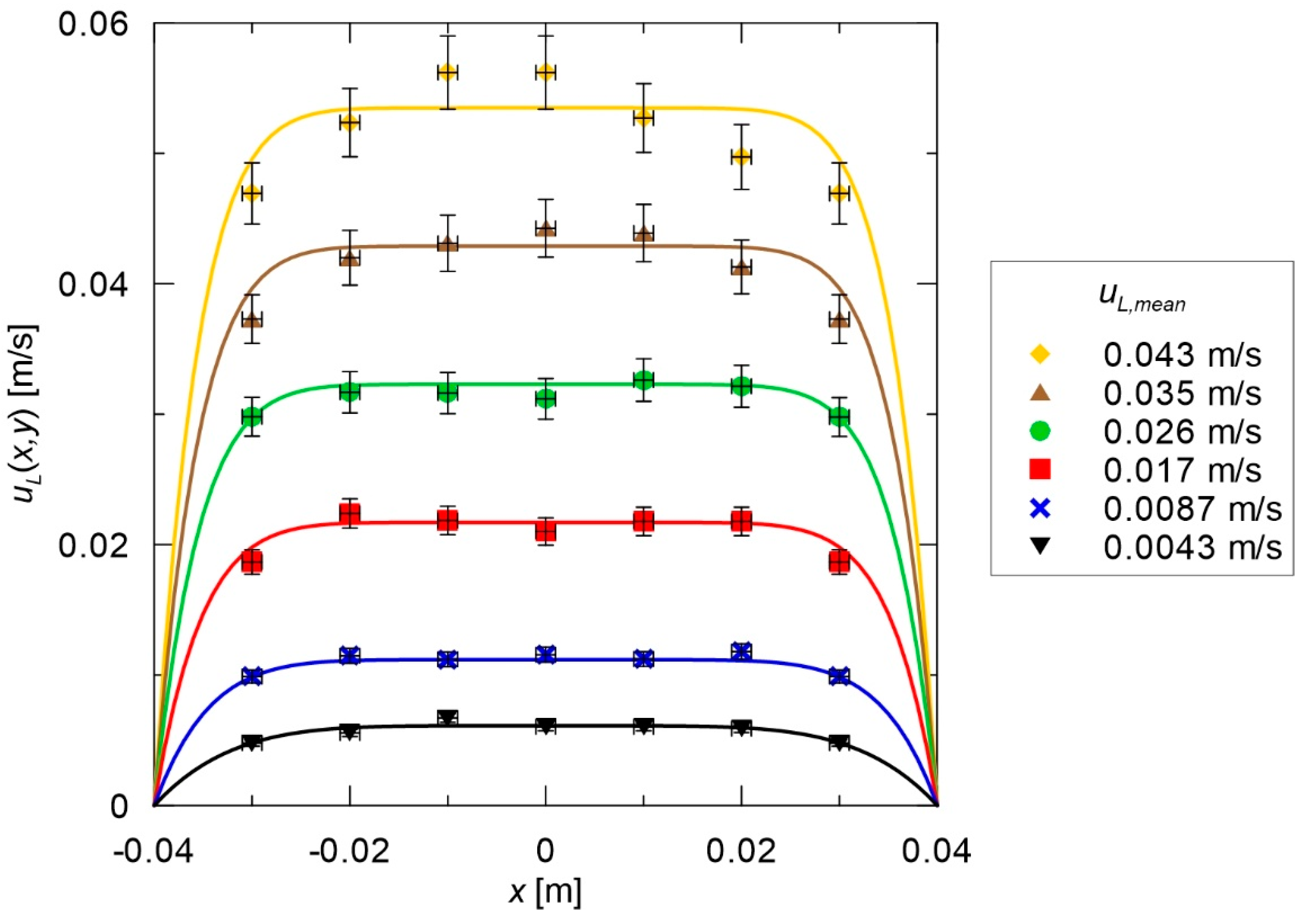
The liquid velocity profile was determined for the average liquid flow velocity in the range of 0.0043–0.043 m/s. For each experimentally obtained velocity profile, the experimental data were approximated using Equation (35). The results obtained are shown in Figure 2. The local velocity of the fluid flowing on the wall was assumed to be equal to zero (no slip conditions). The assumption was confirmed experimentally by injecting the tracer near the wall. The part of the tracer that was in direct contact with the apparatus wall was practically motionless. Velocity at a distance smaller than 0.01 m from the wall was not determined, because a large value of the velocity gradient would cause high uncertainty of the obtained results. The experiments confirmed that the velocity profile approached the plug flow velocity profile. At the same time, the experiments also confirmed that the liquid flow was laminar because the introduced tracer cloud was practically not affected by cross-mixing.
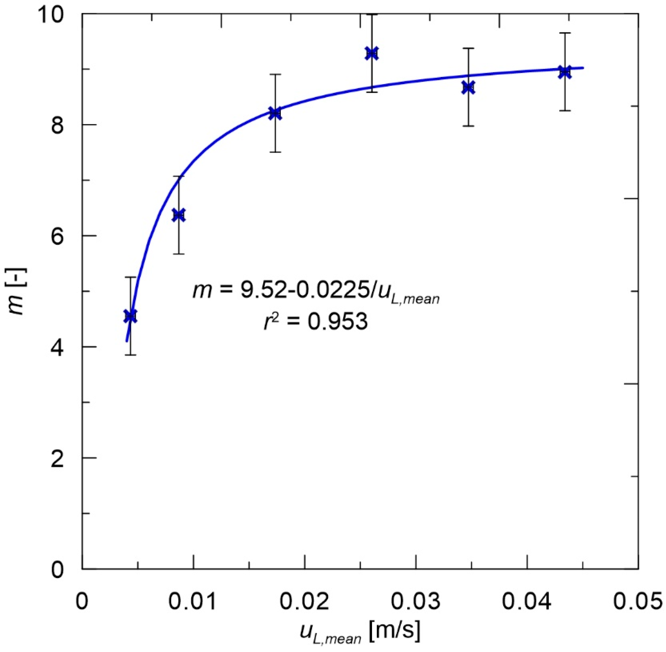
After determining the value of the parameter (Equation (35)) for each examined average liquid velocity, the obtained results were regressed to determine the dependence of on the average liquid velocity, . Along with the parameter, its confidence interval was calculated. For each individual parameter value, the 95% confidence level interval was calculated. For each value it was less than ± 0.7. It could be observed in Figure 3 that the value of the parameter asymptotically tended to be a certain constant value. Assuming that the value of was inversely proportional to the average liquid velocity, and by regressing the obtained data using the equation of type (Figure 3), the following formula was obtained:
Determination of the formula describing the liquid velocity profile permitted the calculation of the local velocity at any point in the apparatus cross-section, without needing to re-measure the local velocity. However, it should be noted, that the proposed Equation (36) was only valid for a particular apparatus design. In order to apply the equation to another type of apparatus, it was necessary to re-run the experiments for a new case and reformulate the equation.
3.2. Drag Coefficient
The drag coefficient was determined using three different reference surfaces defined by Equations (28)–(30). The value of the coefficient was correlated with the Reynolds number for the bubble formed in the flowing liquid. Three different definitions of the characteristic dimension (Equations (31)–(33)) were also employed in the calculation of the Reynolds number. In order to establish the definition that allowed for the most accurate representation of the value of the drag coefficient, , a regression of experimental data was performed using all available combinations of equations. The following power model was adopted for regression:
This model is the one used most often in correlations expressing the value of the drag coefficient, , as a function of the number. Given three different definitions of the characteristic dimensions, three possible reference surface nine correlation equations were obtained. The assessment of the quality of the fit was based on the value of the coefficient of determination, , which was calculated for each case. In statistics, this is used to determine the quality of data representation by means of an analyzed mathematical model. The closer the value was to 1, the better the model fit the experimental data. The results obtained are presented in Table 3.
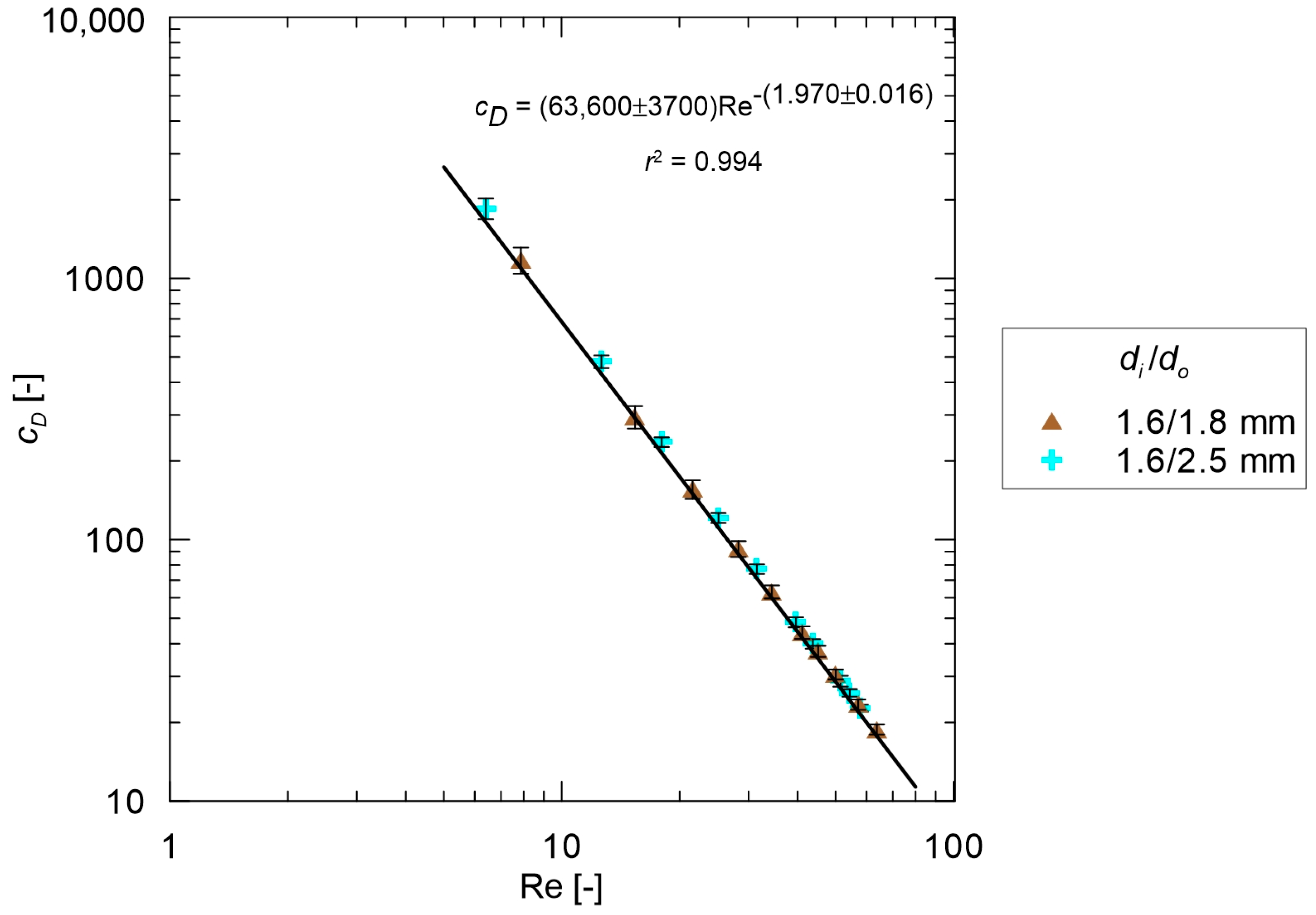
The best fit was obtained for the definition of the drag coefficient, , referring to the cross-sectional area of the bubble (28), and the equivalent diameter of the annulus limited by the diameter of the bubble and the internal nozzle diameter used as the characteristic length in the Reynolds number (32). This case for different internal and external diameters of the nozzle is shown in Figure 4. For the remaining combinations of Equations (28)–(30) and (31)–(33), the individual data series for each nozzle diameter were arranged in parallel series in the resulting graphs, making the model fit much worse than in the case shown in Figure 4.
Based on the combination of definitions given by Equations (28) and (32) and the data shown in Figure 4, the following form of the expression, which allowed the determination of the value of the drag coefficient, , as a function of the Reynolds number was obtained:
In Figure 5, part of the experimental data for the two nozzles with identical internal diameter ( = 1.6 mm) and differing by wall thicknesses, are shown. In the first case, the wall was 0.1 mm thick and in the second one it was 0.45 mm thick. It could be observed that despite large difference in the wall thickness (especially compared to the inner diameter of the nozzle), the results obtained were in line. In fact, none of the used model equations accounted for the outer diameter of the nozzle, so it could be concluded that in the analyzed case, it did not affect the value of the drag coefficient, .
3.3. Comparison with Drag Coefficient Calculated Using the Equation for Bubble Rising
In the scientific literature, there exist many correlations for calculation of the drag coefficient for single bubbles rising in a stagnant liquid. Tomiyama et al. [28] proposed the following formula for bubbles rising in a pure liquid:
Equation (33) was validated in the wide range of experimental conditions and was valid for , , and .
The values of the drag coefficient, , calculated using Equation (28) were then compared with the values obtained from Equation (39) proposed by Tomiyama et al. [28]. The results of the comparison are shown in Figure 6. It could be observed here that the values of the drag coefficient calculated using the proposed Equation (28) differed, even by several orders of magnitude, from the values calculated from Equation (39). In fact, the experimentally derived values of the drag coefficient were much higher than those calculated from the equation used for bubbles rising in a stagnant liquid. This meant that in the case of bubbles forming in the flowing liquid, correlations accounting for the liquid flow must be used.
3.4. Validation of Experimental Drag Coefficient Correlation
In order to verify the obtained results, the correlation derived for (38) was used to calculate the diameter of gas bubbles forming in the concurrently flowing liquid. For this purpose, Equation (28) was introduced into the correlation for the drag coefficient, , given by Equation (38) and the definition of the Reynolds number (Equation (32)). The final form of the obtained equation could be written as:
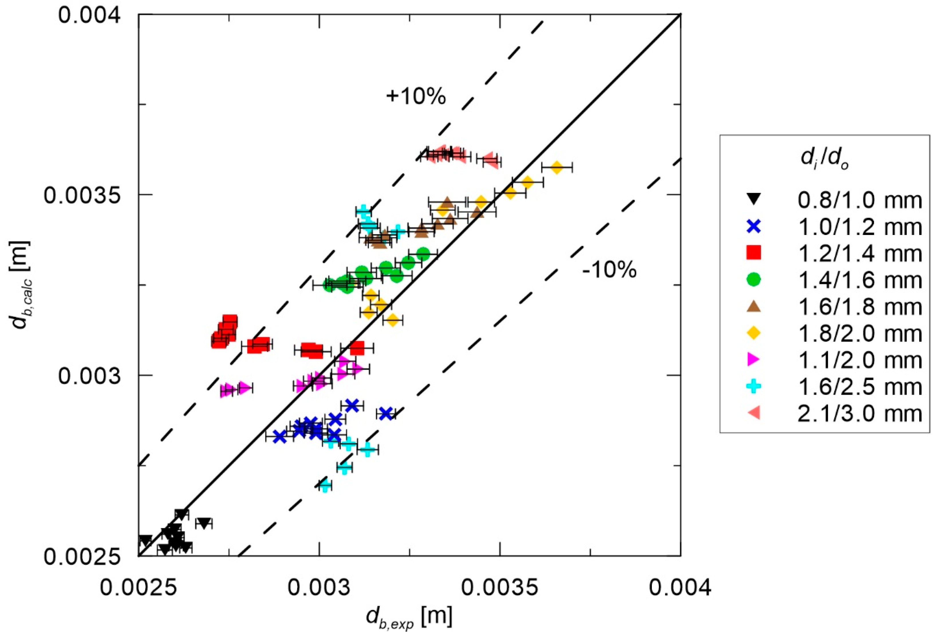
The above equation is a polynomial in which the exponents were real numbers. To determine the diameter of bubbles using Equation (40), it was necessary to solve this using numerical methods. A comparison of the calculated (using “fzero” function of Matlab) and the experimentally determined diameters is shown in Figure 7. It can be seen that most of the results were in very good agreement with the proposed model. The discrepancy between the experimental and calculated results was less than 10% in most cases.
4. Discussion
In this study, an empirical correlation that allows to determine the drag coefficient, , for bubbles formed in the coflowing liquid was derived. It was shown, that even very low liquid flow velocity significantly reduced the diameter of the bubbles, as compared to bubbles forming in a stagnant liquid. The obtained correlation differed significantly from the equations used to determine the drag coefficient, , for the bubble rising in the stagnant liquid. The main reason was a slightly different flow mechanism. When the gas bubbles rose in the stagnant liquid, the rising velocity and bubble diameter were closely related. A bubble of a given diameter rose in the liquid phase at one specific velocity. If the bubbles formed in the flowing liquid, the velocity of this liquid could be changed arbitrarily and the bubble rise velocity would not depend directly on the diameter of the bubble any longer. Moreover, when the bubble was attached to the nozzle, the velocity distribution was slightly different, as in the case of a freely rising bubble. In addition, bubbles with a diameter larger than 1 mm, usually rose along zigzag or spiral flow paths, which could also affect the average drag coefficient value.
The process through which the reference surface should be defined in the terms referring to the drag force, was also specified in this study. Until now, various authors suggested different definitions, depending on the assumptions made. A similar situation applied to the definition of the characteristic length in the Reynolds number definition. The results of the study suggested that the impact of the drag force should be related to the cross-sectional area of the bubble. The Reynolds number should be calculated based on the equivalent diameter of the annulus, limited by the diameter of the bubble and the internal diameter of the nozzle, i.e., .
Additionally, the results presented indicate that in the studied range of nozzle diameters, the nozzle wall thickness practically did not affect the value of the drag coefficient, . In the case of larger wall thicknesses, this effect would probably start to manifest, however, for thin-walled tubes, even up to 4.5x increase in wall thickness did not cause a noticeable effect on the value of the factor.
The diameters of the bubbles calculated using the proposed model based on the force balance and the obtained correlation describing the relationship between the drag coefficient, , and the value of the number, were also validated against experimental results. The calculated bubble diameters proved to be in good agreement with the experimental data, which confirmed the correctness of the proposed model.
The next step might consist of performing measurements for a wider variability range of the process parameters. Apparatuses used in industry often achieve liquid velocities higher than those tested in this work. The frequency of gas bubble formation was selected so that its impact on the diameters of the resulting gas bubbles was as small as possible, however, a much higher gas bubble formation frequency occur in industry. Thus, testing a wider range of gas flow rates might be another parameter to be analyzed.
Author Contributions
Conceptualization, M.P.; methodology, P.L. and M.P.; software, M.P.; validation, P.L. and M.P.; formal analysis, P.L. and M.P.; investigation, P.L.; resources, M.P.; writing—original draft preparation, P.L. and M.P.; writing—review and editing, P.L. and M.P.; visualization, M.P.; supervision, M.P.; funding acquisition, M.P. All authors have read and agreed to the published version of the manuscript.
Funding
The research was supported by subsidy of the Ministry of Science and Higher Education of Poland for Cracow University of Technology in the year 2020.
Conflicts of Interest
The authors declare no conflict of interest. The funders had no role in the design of the study; in the collection, analyses, or interpretation of data; in the writing of the manuscript, or in the decision to publish the results.
Nomenclature
| Symbols: | |
| area of influence of drag force, m2 | |
| , | coefficients, - |
| Bond number, - | |
| drag coefficient, - | |
| conversion factor for conversion diameter in pixels to meters, m/pixel | |
| bubble diameter, m | |
| horizontal bubble diameter, m | |
| inner nozzle diameter, m | |
| outer nozzle diameter, m | |
| bubble detachment frequency, Hz | |
| Froude number, - | |
| modified Froude number (Sada et al. [22]), - | |
| gravitational acceleration, m/s2 | |
| column width, m | |
| mass, kg | |
| coefficient depending on the velocity profile shape, - | |
| gas volumetric flow rate, m3/s | |
| Reynolds number, - | |
| bubble projection surface, pixels | |
| displacement of the center of mass of the bubble, m | |
| time, s | |
| superficial liquid velocity, m/s | |
| gas velocity, m/s | |
| liquid velocity, m/s | |
| mean liquid velocity in the column, m/s | |
| tracer settling velocity, m/s | |
| volume, m3 | |
| , | location coordinates in the column cross-section relative to the column axis, m |
| Greek Symbols: | |
| liquid dynamic viscosity coefficient, Pa·s | |
| gas density, kg/m3 | |
| liquid density, kg/m3 | |
| liquid surface tension, N/m | |
References
- Brennen, C.E.; Brennen, C.E. Fundamentals of Multiphase Flow; Cambridge University Press: New York, NY, USA, 2005. [Google Scholar]
- Curds, C.R. The ecology and role of protozoa in aerobic sewage treatment processes. Ann. Rev. Microbiol. 1982, 36, 27–28. [Google Scholar] [CrossRef]
- Pronk, M.; De Kreuk, M.K.; De Bruin, B.; Kamminga, P.; Kleerebezem, R.V.; Van Loosdrecht, M.C.M. Full scale performance of the aerobic granular sludge process for sewage treatment. Water Res. 2015, 84, 207–217. [Google Scholar] [CrossRef]
- Hasan, M.N.; Khan, A.A.; Ahmad, S.; Lew, B. Anaerobic and aerobic sewage treatment plants in Northern India: Two years intensive evaluation and perspectives. Environ. Technol. Innov. 2019, 15, 100396. [Google Scholar] [CrossRef]
- Besagni, G.; Inzoli, F.; Ziegenhein, T. Two-phase bubble columns: A comprehensive review. ChemEngineering 2018, 2, 13. [Google Scholar] [CrossRef] [Green Version]
- Merchuk, J.C. Airlift bioreactors: Review of recent advances. Can. J. Chem. Eng. 2003, 81, 324–337. [Google Scholar] [CrossRef]
- Prończuk, M.; Bizon, K.; Grzywacz, R. Experimental investigations of hydrodynamic characteristics of a hybrid fluidized bed airlift reactor with external liquid circulation. Chem. Eng. Res. Des. 2017, 126, 188–198. [Google Scholar] [CrossRef]
- Prończuk, M.; Bizon, K. Investigation of the liquid mixing characteristic of an external-loop hybrid fluidized-bed airlift reactor. Chem. Eng. Sci. 2019, 210, 115231. [Google Scholar] [CrossRef]
- Kulkarni, A.A.; Joshi, J.B. Bubble Formation and bubble rise velocity in gas-liquid systems: A review. Ind. Eng. Chem. Res. 2005, 44, 5873–5931. [Google Scholar] [CrossRef]
- Clift, R.; Grace, J.R.; Weber, M.E. Bubbles, Drops, and Particles; Courier Corporation: North Chelmsford, MA, USA, 2005. [Google Scholar]
- Sarkar, M.S.K.A.; Evans, G.M.; Donne, S.W. Bubble size measurement in electroflotation. Miner. Eng. 2010, 23, 1058–1065. [Google Scholar] [CrossRef]
- Besagni, G.; Brazzale, P.; Fiocca, A.; Inzoli, F. Estimation of bubble size distributions and shapes in two-phase bubble column using image analysis and optical probes. Flow Meas. Instrum. 2016, 52, 190–207. [Google Scholar] [CrossRef]
- Wenyuan, F.; Youguang, M.; Shaokun, J.; Ke, Y.; Huaizhi, L. An experimental investigation for bubble rising in non-Newtonian fluids and empirical correlation of drag coefficient. J. Fluid Eng. 2010, 132, 021305. [Google Scholar] [CrossRef]
- Yan, X.; Jia, Y.; Wang, L.; Cao, Y. Drag coefficient fluctuation prediction of a single bubble rising in water. Chem. Eng. J. 2017, 316, 553–562. [Google Scholar] [CrossRef]
- Maldonado, M.; Quinn, J.J.; Gomez, C.O.; Finch, J.A. An experimental study examining the relationship between bubble shape and rise velocity. Chem. Eng. Sci. 2013, 98, 7–11. [Google Scholar] [CrossRef]
- Liu, L.; Yan, H.; Zhao, G.; Zhuang, J. Experimental studies on the terminal velocity of air bubbles in water and glycerol aqueous solution. Exp. Therm. Fluid Sci. 2016, 78, 254–265. [Google Scholar] [CrossRef]
- Patel, S.A.; Glasgow, L.A.; Erickson, L.E.; Lee, C.H. Characterization of the downflow section of an airlift column using bubble size distribution measurements. Chem. Eng. Commun. 1986, 44, 1–20. [Google Scholar] [CrossRef]
- Wongsuchoto, P.; Charinpanitkul, T.; Pavasant, P. Bubble size distribution and gas-liquid mass transfer in airlift contactors. Chem. Eng. J. 2003, 92, 81–90. [Google Scholar] [CrossRef]
- Ruen-ngam, D.; Wongsuchoto, P.; Limpanuphap, A.; Charinpanitkul, T.; Pavasant, P. Influence of salinity on bubble size distribution and gas–liquid mass transfer in airlift contactors. Chem. Eng. J. 2008, 141, 222–232. [Google Scholar] [CrossRef]
- Chuang, S.C.; Goldschmidt, V.W. Bubble formation due to a submerged capillary tube in quiescent and coflowing streams. J. Basic Eng. 1970, 92, 705. [Google Scholar] [CrossRef]
- Terasaka, K.; Tsuge, H.; Matsue, H. Bubble Formation in Cocurrently Upward Flowing Liquid. Can. J. Chem. Eng. 1999, 77, 458–464. [Google Scholar] [CrossRef]
- Sada, E.; Yasunishi, A.; Katoh, S.; Nishioka, M. Bubble formation in flowing liquid. Can. J. Chem. Eng. 1978, 56, 669. [Google Scholar] [CrossRef]
- Muilwijk, C.; Van den Akker, H.E.A. Experimental investigation on the bubble formation from needles with an without liquid co-flow. Chem. Eng. Sci. 2019, 202, 318–335. [Google Scholar] [CrossRef]
- IDS UI-3130CP Rev. 2. Available online: https://en.ids-imaging.com/store/ui-3130cp-rev-2.html (accessed on 12 July 2020).
- Zaruba, A.; Krepper, E.; Prasser, H.M.; Vanga, B.R. Experimental study on bubble motion in a rectangular bubble column using high-speed video observations. Flow Meas. Instrum. 2005, 16, 277–287. [Google Scholar] [CrossRef]
- Nishino, K.; Kato, H.; Torii, K. Stereo imaging for simultaneous measurement of size and velocity of particles in dispersed two-phase flow. Meas. Sci. Technol. 2010, 11, 633. [Google Scholar] [CrossRef]
- Shah, R.K.; London, A.L. Laminar Flow Forced Convection in Ducts: A Source Book for Compact Heat Exchanger Analytical Data; Academic Press: New York, NY, USA, 1978. [Google Scholar]
- Tomiyama, A.; Kataoka, I.; Zun, I.; Sakaguchi, T. Drag coefficients of single bubbles under normal and micro gravity conditions. JSME Int. J. Ser. B Fluids Therm. Eng. 1998, 41, 472–479. [Google Scholar] [CrossRef]
Figure 1.
Schematic drawing of the experimental setup. 1—bubbling zone, 2—liquid valve, 3—rotameter, 4—water inlet, 5—Raschig rings, 6—flow straighteners, 7—air compressor, 8—air valve, 9—orifice, 10—water and air outlet, 11—high fps camera connected to PC, and 12—LED backlight.
Figure 1.
Schematic drawing of the experimental setup. 1—bubbling zone, 2—liquid valve, 3—rotameter, 4—water inlet, 5—Raschig rings, 6—flow straighteners, 7—air compressor, 8—air valve, 9—orifice, 10—water and air outlet, 11—high fps camera connected to PC, and 12—LED backlight.
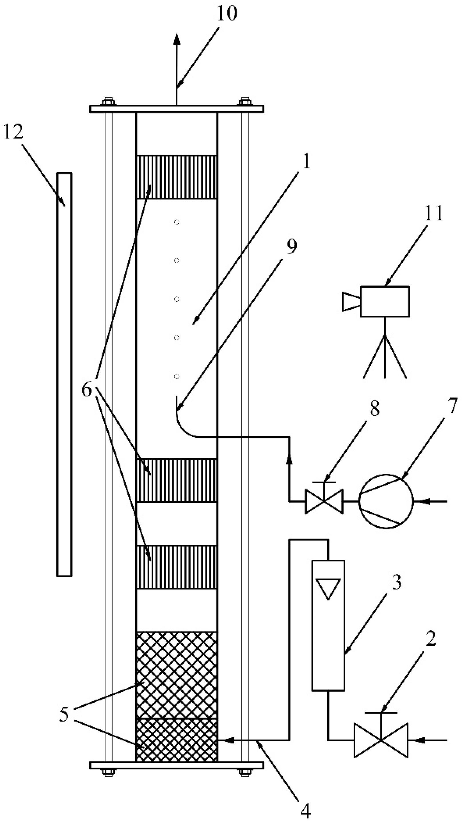
Figure 2.
Liquid velocity profiles for various mean liquid flow velocity; the points represent experimental data and the solid lines represent the calculated velocity profiles.
Figure 2.
Liquid velocity profiles for various mean liquid flow velocity; the points represent experimental data and the solid lines represent the calculated velocity profiles.

Figure 3.
Value of the parameter versus mean liquid velocity, .

Figure 4.
Drag coefficient, , (28) versus Reynolds number (32).

Figure 5.
Drag coefficient, , (28) versus Reynolds number (32) for two nozzles with identical inner diameter ( 1.6 mm) and two different values of outer diameter ( 1.8 mm and 2.5 mm).
Figure 5.
Drag coefficient, , (28) versus Reynolds number (32) for two nozzles with identical inner diameter ( 1.6 mm) and two different values of outer diameter ( 1.8 mm and 2.5 mm).

Figure 6.
Comparison of drag coefficient, , calculated using Equation (28) versus drag coefficient calculated using Equation (39).
Figure 6.
Comparison of drag coefficient, , calculated using Equation (28) versus drag coefficient calculated using Equation (39).
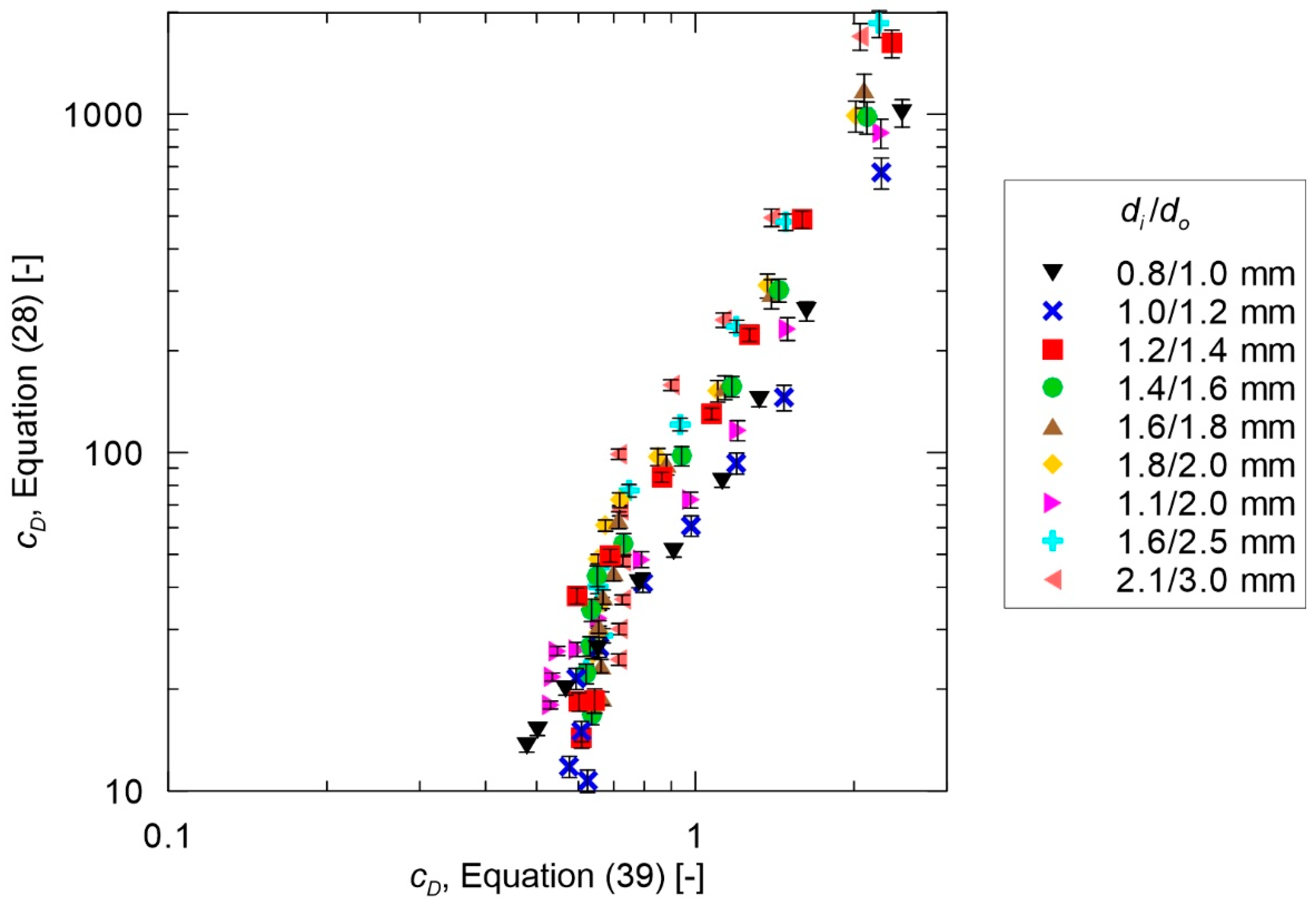
Figure 7.
Comparison of experimental and calculated data, using Equation (40) bubble diameters.


Table 1.
Physical properties of the gas phase (air at 15 °C) and the liquid phase (water at 10 °C).
| Parameter | Symbol | Value |
|---|---|---|
| Gas density | 1.23 kg/m3 | |
| Liquid density | 1000 kg/m3 | |
| Liquid viscosity | 1.31 10−3 Pa·s | |
| Liquid surface tension | 7.42 10−2 N/m |
Table 2.
Nozzle diameters.
| Nozzle Number | Symbol | ||
|---|---|---|---|
| I | 0.8/1.0 | 0.80 ± 0.01 | 1.00 ± 0.01 |
| II | 1.0/1.2 | 1.00 ± 0.01 | 1.20 ± 0.01 |
| III | 1.2/1.4 | 1.20 ± 0.01 | 1.40 ± 0.01 |
| IV | 1.4/1.6 | 1.40 ± 0.01 | 1.60 ± 0.01 |
| V | 1.6/1.8 | 1.60 ± 0.01 | 1.80 ± 0.01 |
| VI | 1.8/2.0 | 1.80 ± 0.01 | 2.00 ± 0.01 |
| VII | 1.1/2.0 | 1.10 ± 0.01 | 2.00 ± 0.02 |
| VIII | 1.6/2.5 | 1.60 ± 0.01 | 2.50 ± 0.02 |
| IX | 2.1/3.0 | 2.10 ± 0.01 | 3.00 ± 0.02 |
Table 3.
Coefficient of determination, , for different combinations of drag coefficient, , and Reynolds number, , definitions.
Table 3.
Coefficient of determination, , for different combinations of drag coefficient, , and Reynolds number, , definitions.
| (28) | (29) | (30) | ||
|---|---|---|---|---|
| (31) | 0.916 | 0.861 | 0.709 | |
| (32) | 0.994 | 0.987 | 0.903 | |
| (33) | 0.727 | 0.772 | 0.936 | |
© 2020 by the authors. Licensee MDPI, Basel, Switzerland. This article is an open access article distributed under the terms and conditions of the Creative Commons Attribution (CC BY) license (http://creativecommons.org/licenses/by/4.0/).
Share and Cite
MDPI and ACS Style
Luty, P.; Prończuk, M. Determination of a Bubble Drag Coefficient during the Formation of Single Gas Bubble in Upward Coflowing Liquid. Processes 2020, 8, 999. https://doi.org/10.3390/pr8080999
AMA Style
Luty P, Prończuk M. Determination of a Bubble Drag Coefficient during the Formation of Single Gas Bubble in Upward Coflowing Liquid. Processes. 2020; 8(8):999. https://doi.org/10.3390/pr8080999
Chicago/Turabian StyleLuty, Przemysław, and Mateusz Prończuk. 2020. "Determination of a Bubble Drag Coefficient during the Formation of Single Gas Bubble in Upward Coflowing Liquid" Processes 8, no. 8: 999. https://doi.org/10.3390/pr8080999
Note that from the first issue of 2016, this journal uses article numbers instead of page numbers. See further details here.