Application of Parameter Optimization to Search for Oscillatory Mass-Action Networks Using Python


Department of Bioengineering, University of Washington, Seattle, WA 98105, USA
*
Author to whom correspondence should be addressed.
Processes 2019, 7(3), 163; https://doi.org/10.3390/pr7030163
Submission received: 21 February 2019
/
Revised: 11 March 2019
/
Accepted: 13 March 2019
/
Published: 18 March 2019
(This article belongs to the Special Issue Methods in Computational Biology)
Abstract
:Biological systems can be described mathematically to model the dynamics of metabolic, protein, or gene-regulatory networks, but locating parameter regimes that induce a particular dynamic behavior can be challenging due to the vast parameter landscape, particularly in large models. In the current work, a Pythonic implementation of existing bifurcation objective functions, which reward systems that achieve a desired bifurcation behavior, is implemented to search for parameter regimes that permit oscillations or bistability. A differential evolution algorithm progressively approximates the specified bifurcation type while performing a global search of parameter space for a candidate with the best fitness. The user-friendly format facilitates integration with systems biology tools, as Python is a ubiquitous programming language. The bifurcation–evolution software is validated on published models from the BioModels Database and used to search populations of randomly-generated mass-action networks for oscillatory dynamics. Results of this search demonstrate the importance of reaction enrichment to provide flexibility and enable complex dynamic behaviors, and illustrate the role of negative feedback and time delays in generating oscillatory dynamics.
1. Introduction
Biological systems exhibit dynamic behaviors due to the regulation of metabolites, proteins, or genetic components, and these dynamics are frequently represented by a series of nonlinear equations for the purpose of computational modeling. Dynamical behaviors in biological systems are dependent on motifs within the network, defined by the species interactions and rate laws which construct the overall network topology. However, the behavior of the system is also heavily influenced by the parameter values attributed to rate constants, regulatory elements, and initial concentrations of floating and boundary species in the network, such that the behavior may shift depending on the current parameter regime. When modeling these biological systems, it may be desirable to obtain a particular dynamic behavior to approximate a physiologically-relevant result. Cell cycle oscillations have been studied for decades but underlying mechanisms remain a topic of interest to systems biologists [1]. Neuroscientists are constructing computational models that exhibit complex oscillatory dynamics to explore the effects of parameter variation, which enriches their understanding of disorders like Parkinson’s and could have implications for treatment [2]. Developing such models requires knowledge of the parameter regimes that permit complex dynamic behaviors, and this knowledge is not always available from experimental data. Searching the landscape which defines parameter space can be a computationally-intensive task, as this landscape is N-dimensional, where N represents the number of parameters in the model, causing the search space to expand dramatically as the number of parameters defining the system increases. Algorithms to scan high-dimensional parameter spaces have been developed and extensively researched, using combinations of global and local searches to define the landscape of computational models and estimate model parameters [3,4,5]. Still, there is a need for efficient parameter optimization tools to search for hallmark dynamic behaviors in systems biology.
A tool implemented in C# was previously developed by Chickarmane et al. to optimize parameter values of biological network models defined by systems of nonlinear equations for bifurcation behavior [6]. Using information about the eigenvalues of bifurcated systems, the authors developed objective functions to independently optimize parameters for either Hopf bifurcations, characteristic of oscillatory systems, or for turning point bifurcations, which can lead to bistability [6]. Such functionality would be desirable in a Pythonic computing environment for those interested in modeling biological systems, as Python is a more ubiquitous computer language in the biological sciences, implemented by expert and novice computer scientists alike, is easily-interpreted by the user, and facilitates integration with existing software for modeling and simulation in systems biology. In the current work, bifurcation–evolution software (evolveBifurcation v1.0.0, Seattle, WA, USA, 2019) is developed in which these objective functions are adapted from C# into user-friendly Python code, and global and local optimization algorithms are implemented for parameter evolution in computational models available through the BioModels Database [7]. The bifurcation–evolution software is then employed to search for oscillatory dynamics in populations of randomly-generated mass-action kinetic models of variable size, and oscillatory models discovered during this search are analyzed to understand how a reduced network topology generates oscillations.
2. Materials and Methods
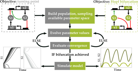
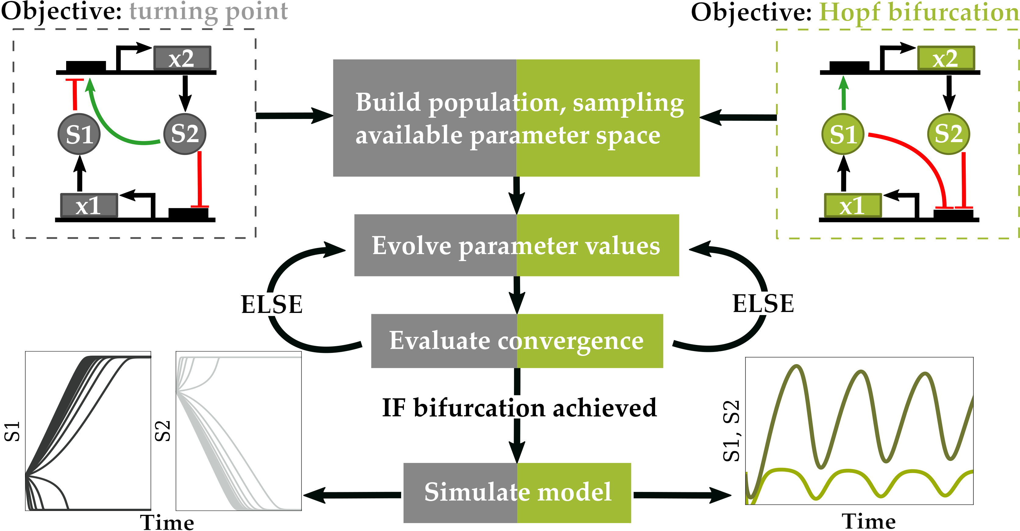
This bifurcation–evolution software relies on standard biological network manipulation and analysis tools available through Tellurium, a Python environment for dynamical modeling of biological networks, and the associated library for simulation of biological models, libRoadRunner [8,9]. The algorithm implemented relies on progressively approximating an acceptable solution to the bifurcation-specific objective function by evolving a population of parameter value vectors. Each parameter vector represents a single point in the landscape of available parameter space that the network can occupy, and vectors which minimize the objective function approximate the global minimum of parameter space, where the desired bifurcation is achieved.
2.1. Objective Function
The objective functions introduced by Chickarmane et al. are re-implemented in the current work, and enable optimization for either switch-like or oscillatory behavior, depending on the bifurcation type selected by the user [6]. Both objective functions rely on intrinsic properties of eigenvalues corresponding to the parameter set governing a system of nonlinear equations at steady state.
2.1.1. Optimization for Turning Point Bifurcations
Turning point bifurcations, capable of introducing bistability and switch-like behavior, can be discovered by minimizing the following objective function as previously described [6]:
A turning point bifurcation requires that one eigenvalue is zero. This objective function is effective for evolving turning point bifurcations because the numerator, which is the product of all eigenvalues of the system, will force the system to assume eigenvalues that approximate zero during minimization. The denominator introduces a penalty for systems in which all eigenvalues are becoming very small, suggesting they are all moving towards the imaginary axis [6]. includes all eigenvalues except the smallest eigenvalue, so that no penalty results from the system achieving one zero-valued eigenvalue. It is not guaranteed that a turning point bifurcation will be reached. Pitchfork and transcritical bifurcations could also result.
2.1.2. Optimization for Oscillatory Systems
For a Hopf Bifurcation bifurcation, which occurs in an oscillatory system, the following objective function is minimized as previously described [6]:
A Hopf bifurcation requires the real part of one of the complex conjugate eigenvalues to approach zero, which is accounted for in the numerator of the objective function, where corresponds to all real components of eigenvalues that have a non-zero complex component. The denominator enhances optimization for systems that have complex conjugate eigenvalues by awarding a penalty to systems with no imaginary component.
2.1.3. Steady State Solver
Optimizing for either bifurcation requires that the model is at steady state before performing the eigenvalue analysis. Steady state represents the solution to the system of differential equations comprising the model when the rates of change of all species equal zero. In order to bring the system to steady state, the Newton-based solver implemented in this work iterates through all independent floating species in the system and takes a step defined by the following equation:
Boldface denotes matrix and vector quantities. In this equation, the dot product of the inverted Jacobian, , and the rates of change, , define the direction of the step, and the step size, , is selected to gradually approximate the steady state value for each floating species in the network. represents a vector of all independent floating species in the network, and represents a single species in the vector. The step size scalar multiplier is adjusted to ensure that the floating species maintains a positive concentration during the steady state approximation. To ensure that the steady state is reached, the Frobenius norm of the rates of change vector is computed and compared to a predefined tolerance level which approximates zero. If the norm is less than the tolerance level, indicating that the concentrations of floating species are not changing significantly, the steady state is reached.
2.2. Parameter Selection and Value Assignment
Global parameter values, floating species initial concentrations, and boundary species concentrations are optimized in the bifurcation–evolution software. Conserved sum parameters, which arise in biological models due to moiety conservation through reversible cycles, are removed from the optimization routine, enabling flexibility in the selection of species concentrations [10,11,12].
Parameter ranges can be specified by the user or automatically specified within the function by referencing initial values contained in the model when it is passed to the function. If the user specifies the bounds, they must submit a sequence defining the upper and lower bounds for each parameter, such that the length of the sequence is equal to the number of parameters undergoing optimization, N. The sequence is thus specified as follows: [(, ), ..., (, )]. Alternatively, the user can specify that all parameters should fall within a uniform range by setting the parameter range argument equal to [(, )].
If the model submitted for optimization is known to permit the desired bifurcation under an optimal parameter regime, and has been assigned parameter values that are a good approximation for the bifurcation type, the user can choose to omit the parameter assignment. Differential evolution, the global optimization algorithm implemented in the bifurcation evolution tool, performs poorly with large parameter value ranges, so selecting appropriate bounds is critical. To accommodate for this, the automatic selection, which is the default setting in the tool, attempts to narrow the ranges in a generalizable manner. First, the algorithm checks the current parameter value, , in the loaded model, and, if the value is zero, the algorithm creates a range of parameter values from to 10, approximating zero but prohibiting possible failure of the algorithm if the parameter appears in the denominator of a rate law. For parameter values less than or equal to 10, the assigned parameter range is from to 10. All parameter values greater than 10 receive a range from to . The automatic assignment allows appropriate flexibility if the range of suitable parameter values for bifurcation is unknown, but relies on the initial parameter value to provide a suitable estimate. If an appropriate range is available for a given parameter through reliable experimental data, manual assignment may be preferable, particularly if this assignment further narrows the range.
Within the differential evolution global optimization algorithm, parameter values are selected from the assigned ranges using a random uniform distribution, such that it is equally likely to choose any value within the assigned range. As this would greatly reduce the frequency of assigned parameter values less than 1, and possibly prevent a parameter from occupying the ideal parameter space to achieve the desired bifurcation behavior, the algorithm selects from a random uniform log distribution of the parameter ranges for all parameters with an upper bound of 10. This ensures that values across multiple orders of magnitude are equally likely to be selected.
2.3. Differential Evolution Algorithm
In the Pythonic approach to this tool, a simple implementation of the differential evolution algorithm developed by Storn and Price was integrated within the bifurcation module, to perform a search in parameter space for global minima of the objective function [13].
2.3.1. Initializing a Population
The algorithm begins by initializing a population of parameter vectors which represent solutions to the objective function. Parameter space in this multi-dimensional optimization problem contains N dimensions, where N is the number of parameters being optimized. These vectors are populated with elements assigned randomly selected values within the predefined bounds specified for , a single parameter, such that the members in the initial population occupy diverse regions of parameter space. While Pythonic versions of this algorithm have been developed, the version available through the scipy.optimize package, frequently used for similar optimization problems, does not allow unfit members to be discarded from the starting population [14]. This makes optimization inefficient, slows convergence and increases the likelihood that the algorithm will terminate before a sufficient minima is reached. The current implementation of the algorithm discards all members with an objective function evaluation above a predetermined threshold before evolving the population. This threshold value coincides with penalty functions included within the bifurcation objective function so that parameter vectors which do not reach steady state, or which have multiple eigenvalues approaching zero in both the real and complex component, are discarded from the solution.
2.3.2. Recombination
During a single round of differential evolution, each member of the population undergoes recombination to construct a trial vector. While iterating through each element, the trial vector is populated with parameter values taken from the member at the current population index or from a mutant vector. If a random number chosen from between zero and one is smaller than the crossover probability, the trial vector receives the parameter value from the mutant vector, as long as the parameter value remains within the acceptable range. Otherwise, the trial vector receives the element from the current population member.
2.3.3. Mutation
Mutated parameter values are generated using the following algebraic expression where boldface denotes vector quantities:
The expression shows that the trial vector element , where i designates the index of the parameter value being mutated, is the sum of a population member element and the scaled difference between two additional population member elements, . The three vectors correspond to randomly selected members of the population that won a single round of tournament selection. The winner of tournament selection is the parameter value vector that has a lower objective function evaluation. While each tournament selection is between population members sampled without replacement, the selection of vectors for mutation between rounds of tournament selection allows sampling with replacement. As a result, vectors may be identical. F is the mutation constant, and can be specified by the user.
2.3.4. Selection
Once the trial member is constructed, the fitness of the member is evaluated. If the trial member has a lower objective function evaluation than the original member at the current population index, the trial member is more fit and selected to replace the original member in the population.
2.3.5. Termination
After the entire population of parameter vectors has undergone recombination, the stopping criteria are assessed to determine if the population has converged on a solution. Termination of differential evolution is achieved when the maximum number of generations has been reached or when the threshold value is met. The threshold value can be selected to consider the smallest eigenvalue of the system, such that the eigenvalue must be sufficiently close to zero to have reached the bifurcation behavior, or the threshold value will correspond to the best objective function fitness from all members in the population. The fitness threshold is the default stopping criteria.
2.3.6. Conditions for Optimal Convergence
There are several input parameters to the differential evolution algorithm that can be manipulated to shift the balance between fast and accurate convergence. Generally, increasing the population size and mutation constant while decreasing the recombination constant will improve the chance that the algorithm converges on a global minimum. However, this will result in computational costs that slow convergence. A population size of 50, and mutation and recombination constants of 0.5, are assigned as default values for the algorithm and typically enable rapid convergence on a suitable solution.
2.4. Local Optimization Algorithm
Following the differential evolution routine, the objective function can be minimized further using an optional bounded Broyden–Fletcher–Goldfarb–Shanno algorithm to provide a final local optimization step [15,16,17,18]. The algorithm uses approximated Hessian updates that are dependent on the approximate gradient at the point in parameter space where the current parameter vector rests, such that it minimizes in the direction of steepest descent. A one-dimensional line search is implemented to determine the step size. This local optimization dramatically reduces the final objective function evaluation for both oscillators and turning points, often yielding a fitness that is minimized by multiple orders of magnitude. However, this step is not recommended for most Hopf bifurcation optimization problems, as fitness values smaller than frequently correspond to damped oscillatory models.
2.5. Random Network Generation
To determine the frequency of oscillators in random networks, a network generator was used which permitted four types of reactions and variable numbers of floating and boundary species. Floating species are state variables, and therefore the concentrations of these species are variable in time during the course of a simulation [19]. Boundary species are fixed and independent of the model state, and are therefore either constant sources to the system or sinks, constant outputs [19]. The random networks were assigned simple mass-action kinetic rate laws and included the reactions summarized in Figure 1. Mass-action kinetic rate laws are proportional to the concentration of the reactant species in the biochemical reaction. Figure 1 therefore defines the mass-action rate laws, , used in the random network generator as the product of a rate constant, k, and the concentration of the reactants involved. Species concentrations are represented by placing brackets around the species name. The generator excludes reactions that violate moiety conservation, and requires that at least one species is a boundary species. For the purpose of analysis of networks with a specified number of species and reactions, which are discussed in the frequency analysis, only networks which did not have orphaned species and which had at least three floating species were passed to the final populations. Three floating species was selected as the minimum cutoff because the smallest system exhibiting a Hopf bifurcation contained three floating species [20]. For parameter value assignment, the random network generator assigned concentrations and rate constants with arbitrary units (a.u). Initial concentrations ranged from 1 to 10 a.u., and rate constants ranged from to 2 a.u. The random network generator was used to create populations of random networks that could be sent to the bifurcation–evolution software to evolve oscillatory dynamics. The default settings in the tool were used for optimization, and, as a result, optimized species initial concentrations ranged from 0.1 to 10.0 a.u., and rate constant value assignments ranged from to 10.0 a.u. Models that could not reach steady state, or which contained negative concentrations, were omitted from analysis. Models that obtained a sufficiently low fitness value after optimization were reset and underwent two additional rounds of optimization to increase the probability of achieving sustained oscillations given an appropriate network architecture, accounting for stochasticity in the algorithm. Following parameter optimization of all networks, populations of a minimum of 1100 randomly-generated networks for each network size were manually assessed for oscillatory dynamics by simulating the model with optimized parameters and inspecting the time-course of all floating species concentrations.
2.6. Machine Specifications
All computations with runtime calculations were performed on an Intel(R) Core(TM) i5-6300HQ CPU (Intel Corporation, Santa Clara, CA, USA) at 2.30 GHz with 8.00 GB RAM.
2.7. Data Repository
All data required to construct the figures in the main text and the bifurcation evolution algorithm sourcecode, evolveBifurcation.py, are publically available on Github. The repository location is provided in the Supplementary Materials.
3. Results
3.1. Testing Bifurcation–Evolution Software on Models from the BioModels Database
To demonstrate the efficacy of the bifurcation–evolution software, models from the BioModels Database underwent parameter optimization for turning point or Hopf bifurcations, depending on the dynamic properties described for each model in the referenced publications. The rate laws describing the models tested are not limited to mass-action kinetics, and demonstrate that the algorithm is effective for optimization of more complex systems. The results of these test cases are shown in Table 1. Graphical output of the optimized networks and model files are available in the supplementary data. Most of these models were tested in the previous work, so we have demonstrated that the Pythonic implementation maintains functionality for all previous test cases [6]. All models were evolved using the default settings in the bifurcation–evolution software, with the exception of the threshold value, which was set independently for turning point and Hopf bifurcations. All turning point models were evolved with a fitness threshold of to induce bistability. All models capable of a Hopf bifurcation were evolved with a fitness threshold of 5 to optimize for oscillatory dynamics. These threshold values were chosen empirically. The runtime is the average number of seconds to complete a single optimization, taken over 100 attempts.
The largest model tested, a negative feedback and bi-rhythmic oscillator containing 10 state variables and 46 global parameters, could achieve oscillatory dynamics after optimization [21]. However, a single run with the default parameters in the bifurcation–evolution software lasted 22 minutes, with the majority of this time allocated to initializing a population of 50 members that could achieve steady state before the differential evolution routine could begin. In some of the simulations of the optimized model, chaotic oscillatory behavior described by the authors arose, which was not observed in any of the other models tested.
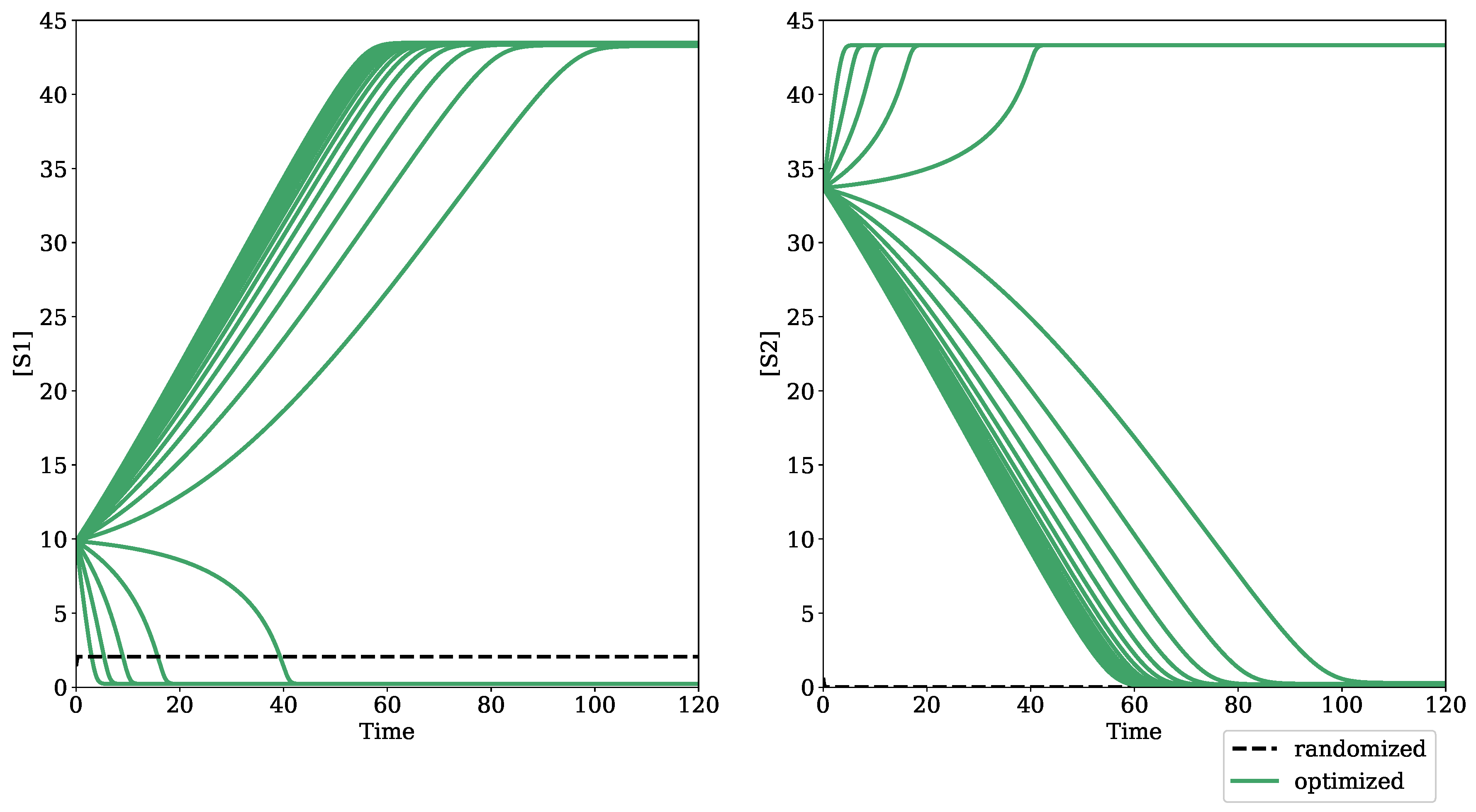
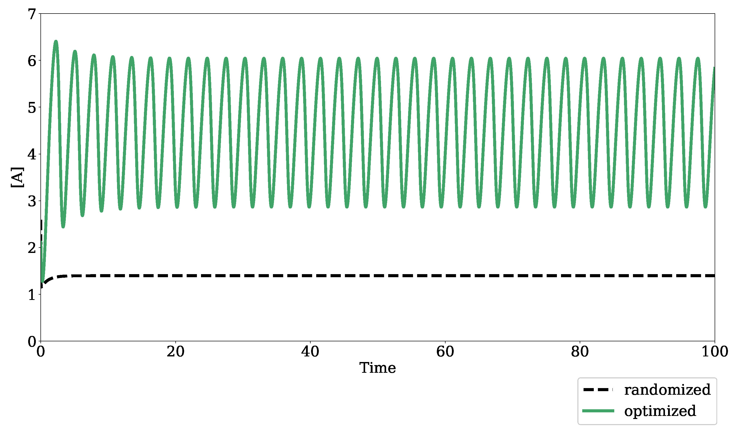
Figure 2 shows the result of optimizing for a turning point bifurcation in the Hervagault bistable switch model [22]. Before parameter optimization, the concentrations of S1 and S2 reach a single steady state despite a parameter sweep in the global parameter, J1_k. After parameter optimization, both S1 and S2 achieve two distinct steady states, demonstrating the bistable dynamics of the model in a parameter regime with eigenvalues that satisfy the condition for a turning point bifurcation. Figure 3 shows the result of optimizing for a Hopf bifurcation in the modified Edelstein relaxation oscillator model [23]. Before parameter optimization, species A reaches a steady state upon simulation. However, once optimized, species A achieves sustained oscillatory dynamics.
3.2. Oscillation Discovery in Randomly-Generated Networks
The bifurcation–evolution software was used to search populations of randomly-generated networks for models exhibiting oscillatory dynamics. Table 2 shows the percentage of sustained oscillators in populations of randomly-generated networks with variable network sizes. Networks either have an equal ratio (1:1) of species to reactions, or are enriched with more reactions than species (1:1.5). Figure 4 shows the frequencies of oscillatory dynamics in networks of variable size. The top row of Figure 4 contains frequency data of all oscillating systems, including those with sustained and damped dynamics. The bottom row contains only the frequency of sustained oscillatory dynamics. The frequency of sustained oscillators increases for larger networks in both the 1:1 and 1:1.5 network sizes. However, networks with a 1:1.5 ratio have a higher frequency of oscillatory dynamics than networks with a 1:1 ratio when comparing networks with the same number of species, therefore increasing the ratio of reactions to species increases the frequency of oscillators in randomly-generated populations.
In Figure 5 and Figure 6, oscillator frequency within a given network size is binned by the number of floating species in the network. All networks tested which exhibited sustained oscillations had a minimum of four floating species. In networks which have an equal number of reactions and species, sustained oscillatory dynamics were only achieved in networks that had fewer than floating species, where n is the total number of species in the network, as shown in Figure 5. As demonstrated by the histograms in Figure 6, for populations with a enrichment in the number of reactions, networks could achieve sustained oscillations with the maximum number of floating species. In most cases, an intermediate number of floating species achieved sustained oscillatory dynamics with the highest frequency for networks with either a 1:1 or 1:1.5 ratio. Enriching the number of reactions shifted the histogram towards higher numbers of floating species. For all network sizes, the spread of the histogram increased when damped oscillators were considered.
3.3. Components of Randomly-Generated Networks Responsible for Oscillation
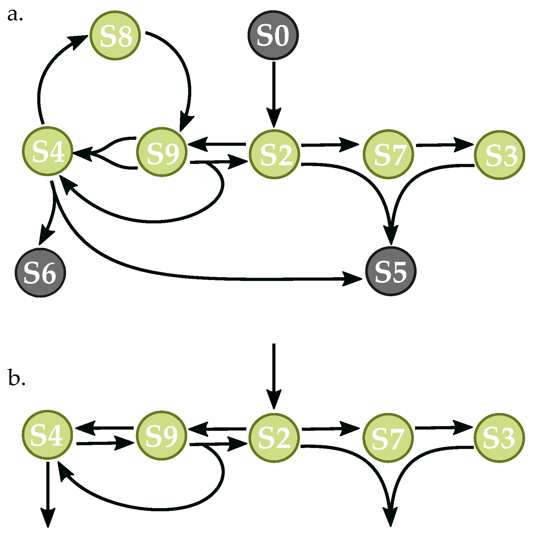
Next, a population of 10,000 randomly-generated 10 species, 10 reaction networks were generated, allowing for the existence of orphaned species, which are disconnected from the network. In addition, of these networks had at least one orphaned species, and the frequency of oscillatory dynamics was greatest in the subset of networks containing orphaned species. Figure 7 and Figure 8 show two randomly-generated networks which were pulled from the population to study the components of the network topology, or species connectivity, responsible for oscillatory dynamics. Both networks have nine total species that participate in reactions, indicating that one of the species was orphaned, and therefore does not contribute to the network dynamics. The reduced forms of these networks, which maintain oscillatory behavior, were generated by removing unnecessary and redundant nodes or reactions, and compounding constant parameters within the rate law. These reduced forms show the species and reactions responsible for oscillatory dynamics.
The reduced network in Figure 7 shows feedback loops that contribute to oscillatory behavior. The first pathway of interest is the sequence of unimolecular–unimolecular reactions from species S1 to S6, with two intermediate nodes, S3 and S5. This pathway shows that, as the concentration of species S1 increases or decreases, there is an impact on species S6 in the same direction of change, accompanied with a time delay in the signal due to the intermediate nodes. Continuing the cycle, an increase in species S6 contributes to a rise in species S2 and subsequent production of S5, feeding back positively into the pathway that produces species S6 and sustaining the cycle. However, negative feedback of S6 on S1 is key for enabling oscillations. While species S6 increases, the bi-molecular reaction between S6 and S1 which produces S2 simultaneously reduces the concentration of species S1 available for the uni-molecular reaction producing species S3. Together, the feedback and time delay promote oscillation. This cycle repeats without dampening given appropriate global parameter values.
The reduced network in Figure 8 also contains feedback loops, involving the reversible reactions between species S2, S9,and S4, as well as the reactions between species S2, S7 and S3. The optimized model drives the conversions of S2 to S9 and S9 to S4 at a fast rate, while the conversion of S4 to S9 occurs much more slowly, as determined by the rate constants for these reactions. Since species S9 feeds back to S4 when generating S2, negative feedback arises. It is important to note that reactions involving S8 effectively promote a time delay due to the involvement of an intermediate node in the production of S2, which impacts the phase of the oscillations. However, removing species S8 allows for a simplified reversible reaction between S4 and S9 in which the time delay created by the intermediate node can be partially compensated for by adjusting the rate constants in the reversible reaction. In the second loop, S3 exerts negative feedback on S2—as the concentration of S3 increases due to greater conversion of S2 to S7, more of species S2 is consumed in the bi-molecular reaction with S3, reducing the production of species S7. Again, species S7 serves to promote a delay in the signal.
4. Discussion
4.1. Algorithm Evaluation
In this paper, a Pythonic interpretation of existing objective functions to evaluate the fitness of system parameters for bifurcation behavior is presented, and a differential evolution algorithm is implemented for progressive parameter optimization. The bifurcation–evolution software relies on iterative minimization of an objective function that rewards networks with eigenvalues approximating the specified bifurcation behavior. Several published models from the BioModels Database were tested, and demonstrated that the algorithm performs well using default conditions for models with few parameters, evolving the desired bifurcation behavior with a short runtime and within a few generations. The bifurcation–evolution software could produce oscillatory dynamics in an mitogen-activated protein kinase feedback oscillator model with 30 parameters (including 22 global parameters and eight state variables) in less than 45 seconds. However, the largest model tested, which contained 56 total parameters for optimization with a Hopf bifurcation objective, required a 22 minute runtime, suggesting that the bifurcation–evolution software may not be efficient for larger models. This extended runtime was attributed to the task of generating an initial population of suitable members, indicating that the randomized parameter value selection created many individuals which could not reach steady state, excluding these parameter sets from the population. It is likely that this model is also sensitive, only reaching steady state and achieving oscillatory dynamics for a small subset of parameter space, such that small changes in parameter values dramatically alter the model dynamics.
The bifurcation–evolution software presents several optional arguments that the user can alter to increase the probability of finding a suitable solution or to expedite convergence, as the stiffness of the model will affect the efficiency of the algorithm converging on a solution. Increasing the mutation constant and population size, or lowering the recombination constant will improve the chance of converging on a global minima. However, these actions will also increase the time required for convergence. For larger models which complicate the steady state solver computation, it may be desirable to decrease the population size and increase the maximum number of iterations so that computation time is shifted from initializing the population to performing the evolution routine. Additionally, differential evolution is sensitive to parameter ranges. The default settings for parameter range selection attempts to create narrow, parameter-specific ranges while still providing sufficient space for non-trivial randomization. Providing broad ranges will generally reduce the efficiency of the differential evolution algorithm and greatly reduce the chance of converging on a suitable solution. However, the user can further restrict or expand these ranges when appropriate to improve the chance of convergence.
While the results of testing the bifurcation–evolution software on multiple published biological models and on randomly-generated mass-action networks suggest that the algorithm previously implemented by Chickarmane et al. is suitable for detecting turning point and Hopf bifurcations, there are some limitations. The objective function for turning point bifurcations cannot detect bistable systems automatically. Instead, the user must pass the optimized model to external software that permits bifurcation analysis or perform manual parameter scans to search for bistability, as in Figure 1. The Pythonic implementation presented does not distinguish between systems with turning point bifurcations and pitchfork or transcritical bifurcations, so it would be desirable to add an additional step to eliminate parameter sets that correspond to these bifurcation types as in the previous implementation in C#. Similarly, the objective function for Hopf bifurcations still permits damped oscillators to be represented as solutions with good fitness values as determined by the eigenvalues of the optimized parameter set, depending on the stringency of the threshold value. Chaotic oscillatory dynamics also resulted following parameter optimization in a subset of the tested cases in the model of drosophila circadian rhythms by Leloup et al. [21]. While chaos and birhythmicity are known to arise in this model, the presence of these dynamics in the parameter-optimized model suggests that the algorithm does not exclude global bifurcations from the evolving population. While a system with a zero real component of one member of a complex conjugate pair would be a true Hopf bifurcation that produces sustained oscillations, the bifurcation–evolution software only approximates this behavior. Additionally, since the bifurcation–evolution software introduces stochasticity and depends on appropriate parameter ranges for convergence, it is not guaranteed to produce the bifurcation behavior selected on every run. This may require that the function is called multiple times before a satisfactory solution is reached.
4.2. Oscillator Frequency in Randomly-Generated Network Populations
The frequency data presented shows the intuitive result that larger random networks are more likely to contain components that permit oscillatory dynamics. All randomly-generated networks which exhibited sustained oscillations contained at least four floating species, although a system with three floating species could conceivably achieve a Hopf bifurcation with the appropriate network topology [20]. This suggests that oscillatory networks with three floating species are rare in randomly-generated populations and sensitive to the parameter regime, such that oscillatory networks occupy only a small region of parameter space. Oscillatory dynamics arise in networks that have negative feedback and a time delay, as described for the networks in Figure 7 and Figure 8. These are more likely to arise in larger networks because there are more nodes to participate in complex loops and engage in multiple reactions, increasing the likelihood of randomly generating a motif that provides the feedback or time delay architecture. Figure 8 shows that it is advantageous to have a large number of floating species to produce complex dynamics, as the reduced network has two three-species loops that incorporate negative feedback, but the individual loops could not sustain oscillatory dynamics when the second loop was removed. However, the data also suggests that the number of reactions available to floating species in the network exerts greater control over the frequency of oscillatory dynamics than does the total number of species.
Intentionally increasing the ratio of reactions to species greatly increases the frequency of oscillatory dynamics following parameter optimization, as shown by the oscillator enrichment in the 1:1.5 networks shown in Figure 5 compared to the 1:1 networks shown in Figure 4. In the case where the number of reactions and species are equal, as in Figure 4, oscillatory dynamics only appear in networks with fewer than floating species, where n is the total number of boundary and floating species in the network. The networks which produce oscillators tend to have the reaction density shifted onto the floating species, with minimal reaction density between boundary species. This shift creates a local enrichment of reaction density on the floating species, permitting greater control over the dynamic interactions between these species by providing flexibility to the network. This is not necessary in the networks that have a 1:1.5 ratio, in which networks with the maximal number of floating species can give rise to oscillatory dynamics because sufficient flexibility is conferred by the intentional enrichment in the number of reactions. As a result, networks with a 1:1 ratio of total species to reactions can approximate the behavior seen in networks with a 1:1.5 ratio by decreasing the number of floating species in the network and minimizing the number of trivial reactions between boundary species to locally enrich the reaction density between species that contribute to network dynamics. The importance of reaction enrichment is further confirmed by the study of the 10 species, 10 reactions randomly-generated network populations in which orphaned species were permitted. The majority of oscillatory networks in this population included at least one orphaned species, which enriches the reaction density between the remaining species in the network and provides additional flexibility.
Together, these data demonstrate the importance of providing a mass-action network with sufficient connectivity to enable dynamic bifurcation behaviors to arise. True biological systems, which may incorporate complex rate laws involving cooperativity and enzyme kinetics, could circumvent such limitations in network size and reaction enrichment. In addition to the studies presented describing the frequency of oscillatory dynamics, further studies should explore the sizes of the parameter landscapes which permit desired bifurcation behaviors. This could better explain the sensitivity of some optimized networks to variation in the parameter regime, and could provide researchers with a greater understanding of the impact of small perturbations on overall system dynamics. The presented bifurcation evolution tool would facilitate such a study. With this tool, modeling of complex biological systems which exhibit oscillatory dynamics or turning point bifurcations can be readily optimized to achieve such behavior given the appropriate network topology. The tool also facilitates exploration of parameter space in models for which the full range of dynamic behavior is unknown, which could enable detection of rare dynamic behavior inside a small subspace of the parameter landscape and inform experimental studies with possible implications for understanding disease and the molecular underpinnings of life.
5. Conclusions
Biological systems are often described with systems of nonlinear equations to model the dynamics of metabolic, protein, or gene-regulatory networks. While the topology of such models constrains the range of dynamic behavior that can be achieved, parameter regimes that fully define the reaction rates and interactions, as well as the state variables of the system, also determine whether a given dynamic behavior will arise. Locating parameter regimes that induce bifurcations can be challenging due to the size of the parameter landscape. In this work, a Pythonic bifurcation–evolution software is presented which employs existing bifurcation objective functions and a differential evolution algorithm that minimizes these objectives to improve the fitness of the best candidate parameter regime, progressively optimizing the system for either a turning point or Hopf bifurcation. The objective functions reward systems with steady state eigenvalues approximating those characteristic of the desired bifurcation. The bifurcation–evolution software is validated using published models from the BioModels Database, confirming that the algorithm performs well for evolving bistability and oscillations. The bifurcation-evolution software was subsequently used to determine the frequency of oscillators in randomly-generated mass-action network populations, and the results of this search indicate that populations of large random networks with 50% reaction enrichment achieve oscillatory dynamics more frequently than networks with fewer species or with an equivalent number of species and reactions. This demonstrates the importance of reaction enrichment for flexibility that enables complex dynamic behaviors. An analysis of selected randomly-generated mass-action networks from these populations shows that negative feedback and time delays are involved in the generation of oscillatory dynamics. Ultimately, the studies presented in the current work demonstrate the utility of the bifurcation-evolution software for efficiently exploring parameter space for a solution that satisfies the bifurcation objective. Due to the ubiquity of Python in computational biology, this Pythonic bifurcation-evolution software can be readily understood and easily-integrated with existing modeling software, providing the modeling community with a tool that could help detect of rare dynamics and inform experimental studies of disease and the molecular mechanisms underlying a range of biological phenomena.
Supplementary Materials
All supplementary materials required to generate the data and figures in the main text are available at https://github.com/vporubsky/evolve-bifurcation. evolveBifurcation.py contains the sourcecode for the bifurcation evolution algorithm described in the text. Optimized bifurcated BioModels represented in an Antimony string format and time-course simulation output is included for all test cases. All randomly-generated networks are provided in Antimony formats and time-course simulation output for each network is included.
Author Contributions
V.L.P. was responsible for data curation, formal analysis, investigation, methodology, software, validation, visualization, and writing the original manuscript draft. H.M.S. was responsible for conceptualization, funding acquisition, project administration, resources, and assisted in formal analysis and visualization. Both V.L.P. and H.M.S. reviewed and edited the manuscript.
Funding
H.M.S. is very grateful for the support provided by National Institutes of Health grants GM123032-01, U01HL122199-02, and P41EB023912. V.L.P. is grateful for the support of National Institutes of Health grant P41EB023912.
Acknowledgments
V.L.P. would like to thank Kiri Choi for valuable discussions about integrating steady state solvers and the functionality provided by Tellurium and libRoadRunner for implementing the bifurcation evolution algorithm. V.L.P. would also like to thank J. Kyle Medley for providing insight into the utility and shortcomings of several global and local optimization algorithms.
Conflicts of Interest
The authors declare no conflict of interest. The funders had no role in the design of the study; in the collection, analyses, or interpretation of data; in the writing of the manuscript, or in the decision to publish the results.
References
- Csikasz-Nagy, A. Computational systems biology of the cell cycle. Brief. Bioinform. 2009, 10, 424–434. [Google Scholar] [CrossRef] [PubMed] [Green Version]
- Pavlides, A.; Hogan, S.J.; Bogacz, R. Computational Models Describing Possible Mechanisms for Generation of Excessive Beta Oscillations in Parkinson’s Disease. PLoS Comput. Biol. 2015, 1, e1004609. [Google Scholar] [CrossRef] [PubMed]
- Zamora-Sillero, E.; Hafner, M.; Ibig, A.; Stelling, J.; Wagner, A. Efficient characterization of high-dimensional parameter spaces for systems biology. BMC Syst. Biol. 2011, 5, 142. [Google Scholar] [CrossRef] [PubMed]
- Liu, Y.; Gunawan, R. Parameter estimation of dynamic biological network models using integrated fluxes. BMC Syst. Biol. 2014, 8, 127. [Google Scholar] [CrossRef]
- Ashyraliyev, M.; Fomekong-Nanfack, Y.; Kaandorp, J.A.; Blom, J.G. Systems biology: Parameter estimation for biochemical models. FEBS J. 2009, 276, 886–902. [Google Scholar] [CrossRef] [PubMed]
- Chickarmane, V.; Paladugu, S.R.; Bergmann, F.; Sauro, H.M. Bifurcation discovery tool. Bioinformatics 2005, 21, 3688–3690. [Google Scholar] [CrossRef] [Green Version]
- Li, C.; Donizelli, M.; Rodriguez, N.; Dharuri, H.; Endler, L.; Chelliah, V.; Li, L.; He, E.; Henry, A.; Stefan, M.I.; et al. BioModels Database: An enhanced, curated and annotated resource for published quantitative kinetic models. BMC Syst. Biol. 2010, 4, 92. [Google Scholar] [CrossRef]
- Choi, K.; Medley, J.K.; Cannistra, C.; Konig, M.; Smith, L.; Stocking, K.; Sauro, H.M. Tellurium: A Python Based Modeling and Reproducibility Platform for Systems Biology. Biosystems 2018, 171, 74–79. [Google Scholar] [CrossRef]
- Somogyi, E.T.; Bouteiller, J.M.; Glazier, J.A.; König, M.; Medley, J.K.; Swat, M.H.; Sauro, H.M. libRoadRunner: A high performance SBML simulation and analysis library. Bioinformatics 2015, 31, 3315–3321. [Google Scholar] [CrossRef]
- Reich, J.G.; Selkov, E.E. Energy Metabolism of the Cell: A Theoretical Treatise; Academic Press: London, UK, 1981; p. 345. [Google Scholar]
- Sauro, H.M.; Ingalls, B. Conservation analysis in biochemical networks: Computational issues for software writers. Biophys. Chem. 2004, 109, 1–15. [Google Scholar] [CrossRef]
- Sauro, H.M. Systems Biology: An Introduction to Metabolic Control Analysis; Ambrosius Publishing: Seattle, WA, USA, 2018. [Google Scholar]
- Storn, R.; Price, K. Differential Evolution—A Simple and Efficient Heuristic for global Optimization over Continuous Spaces. J. Glob. Optim. 1997, 11, 341–359. [Google Scholar] [CrossRef]
- scipy.optimize.differential_evolution—SciPy v1.1.0 Reference Guide. Available online: https://docs.scipy.org/doc/scipy/reference/generated/scipy.optimize.differential_evolution.html (accessed on 5 November 2018).
- Broyden, C.G. The Convergence of a Class of Double-rank Minimization Algorithms 1. General Considerations. IMA J. Appl. Math. 1970, 6, 76–90. [Google Scholar] [CrossRef]
- Fletcher, R. A new approach to variable metric algorithms. Comput. J. 1970, 13, 317–322. [Google Scholar] [CrossRef] [Green Version]
- Goldfarb, D. A Family of Variable-Metric Methods Derived by Variational Means. Math. Comput. 1970, 24, 23. [Google Scholar] [CrossRef]
- Shanno, D.F. Conditioning of Quasi-Newton Methods for Function Minimization. Math. Comput. 1970, 24, 647. [Google Scholar] [CrossRef]
- Sauro, H.M. Systems Biology: Introduction to Pathway Modeling, 1st ed.; Ambrosius Publishing: Seattle, WA, USA, 2017. [Google Scholar]
- Wilhelm, T.; Heinrich, R. Smallest chemical reaction system with Hopfbifurcation. J. Math. Chem. 1995, 17, 1–14. [Google Scholar] [CrossRef]
- Leloup, J.; Goldbeter, A. Chaos and birhythmicity in a model for circadian oscillations of the PER and TIM proteins in drosophila. J. Theor. Biol. 1999, 198, 445–459. [Google Scholar] [CrossRef]
- Hervagault, O.; Canu, P. Bistability and Irreversible Transitions in a Simple Substrate Cyclet; Technical Report; University of Technology of Compiègne: Compiègne, France, 1987. [Google Scholar]
- Seno, M.; Iwamoto, K.; Sawada, K. Instability and Oscillatory Behavior of Membrane-Chemical Reaction Systems; Technical Report; University of Tokyo: Tokyo, Japan, 1978. [Google Scholar]
- Tyson, J.J.; Chen, K.C.; Novak, B. Sniffers, buzzers, toggles and blinkers: Dynamics of regulatory and signaling pathways in the cell. Curr. Opin. Cell Biol. 2003, 15, 221–231. [Google Scholar] [CrossRef]
- Edelstein, B.B. Biochemical Model With Multiple Steady States and Hysteresis. J. Theor. Biol. 1970, 29, 57–62. [Google Scholar] [CrossRef]
- Angeli, D.; Ferrell, J.E.; Sontag, E.D. Detection of multistability, bifurcations, and hysteresis in a large class of biological positive-feedback systems. Proc. Natl. Acad. Sci. USA 2004, 101, 1822–1827. [Google Scholar] [CrossRef] [Green Version]
- Nicolis, G.; Prigogine, I. Self-Organization in Nonequilibrium Systems; Wiley-Blackwell: Hoboken, NJ, USA, 1977; Volume 82, p. 672. [Google Scholar]
- Heinrich, R.; Rapoport, S.M.; Rapoport, T.A. Metabolic regulation and mathematical models. Proq. Biophys. Mol. Biol. 1977, 32, 1–82. [Google Scholar]
- Kholodenko, B.N. Negative feedback and ultrasensitivity can bring about oscillations in the mitogen-activated protein kinase cascades. Eur. J. Biochem. 2000, 267, 1583–1588. [Google Scholar] [CrossRef] [PubMed] [Green Version]
- Goldbeter, A. A minimal cascade model for the mitotic oscillator involving cyclin and cdc2 kinase. Proc. Natl. Acad. Sci. USA 1991, 88, 9107–9111. [Google Scholar] [CrossRef] [PubMed]
- François, P.; Hakim, V. Core genetic module: The mixed feedback loop. Phys. Rev. E 2005, 72, 031908. [Google Scholar] [CrossRef] [PubMed]
- Lavrentovich, M.; Hemkin, S. A mathematical model of spontaneous calcium(II) oscillations in astrocytes. J. Theor. Biol. 2008, 251, 553–560. [Google Scholar] [CrossRef] [PubMed]
Figure 1.
Types of reactions permitted in randomly-generated networks, governed by laws of mass-action. Reactions are depicted visually and written with standard biochemical reaction formatting. Mass-action kinetic rate laws, , for each reaction are defined by the product of rate constant, k, and the concentrations of reactant species. (a) unimolecular–unimolecular reaction; (b) unimolecular–bimolecular reaction; (c) bimolecular–unimolecular reaction; (d) bimolecular– bimolecular reaction.
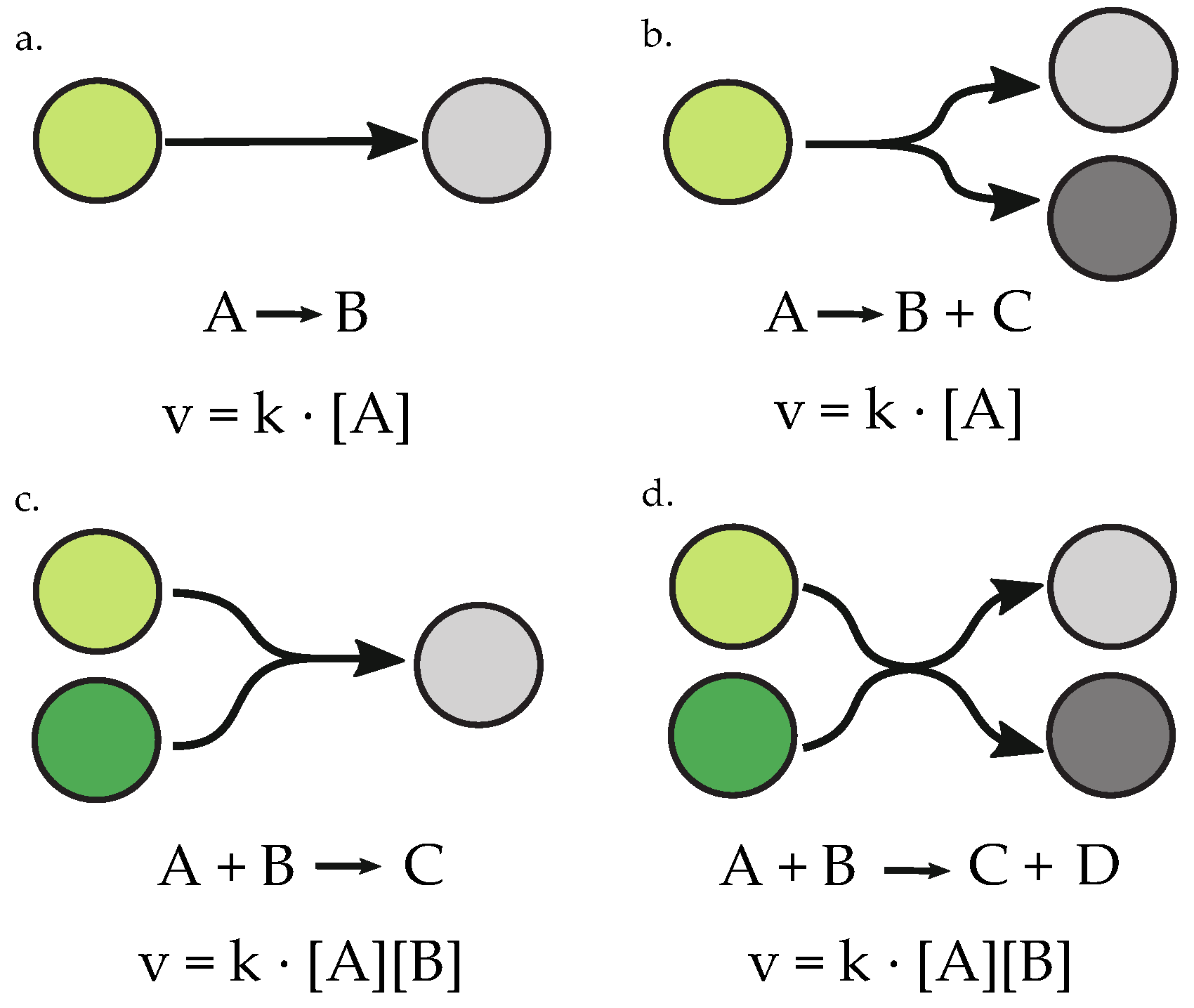
Figure 2.
Optimized dynamic concentration changes in a bistable over time. The dashed black trace is the result randomizing all parameter values in the bistable switch model from Hervagault and Canu, 1987, using Tellurium and libRoadRunner functionalities by selecting from a uniform distribution between 0.001 and 15.0 and performing a parameter sweep of parameter J1_k from 0.0 to 2.0. The green trace is the optimized bistable output for both floating species in the model in response to an identical parameter sweep after the randomized parameters were evolved with default settings in the bifurcation–evolution software.

Figure 3.
Optimized dynamic output of an oscillatory model. The dashed black trace is the result of simulating the modified Edelstein relaxation oscillator from Seno et al., 1978, using Tellurium and libRoadRunner functionalities after randomizing parameter values from a uniform distribution between log(0.01) and log(10.0). The green trace is the optimized oscillatory output after the randomized model underwent parameter evolution with default settings in the bifurcation–evolution software.

Figure 4.
Frequency of occurrence of oscillatory dynamics in populations of randomly-generated networks of variable size, disallowing orphan species. Network sizes are labeled in the form, number of species × number of reactions. Networks either contain an equal ratio of species to reactions (1:1) or a enrichment in the number of reactions (1:1.5). (Top row) frequency of networks exhibiting sustained oscillators and damped oscillators; (Bottom row) frequency of sustained oscillating networks.
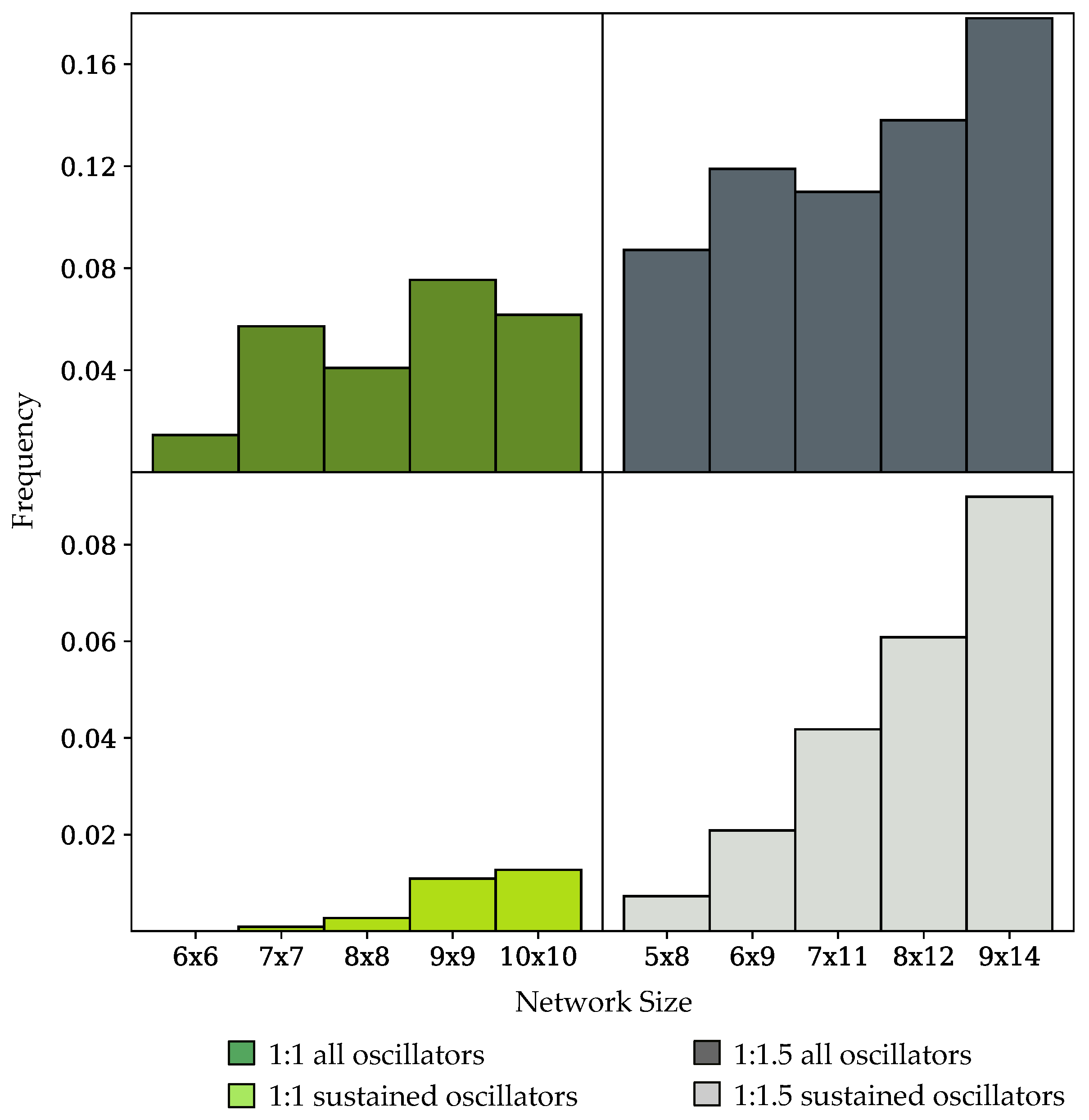
Figure 5.
Frequency of occurrence of oscillatory dynamics in randomly-generated networks with a 1:1, number of species to number of reactions ratio, binned by the number of floating species in the network. (Top row) frequency of oscillatory dynamics, including sustained and damped systems; (Bottom row) frequency of sustained oscillatory dynamics.
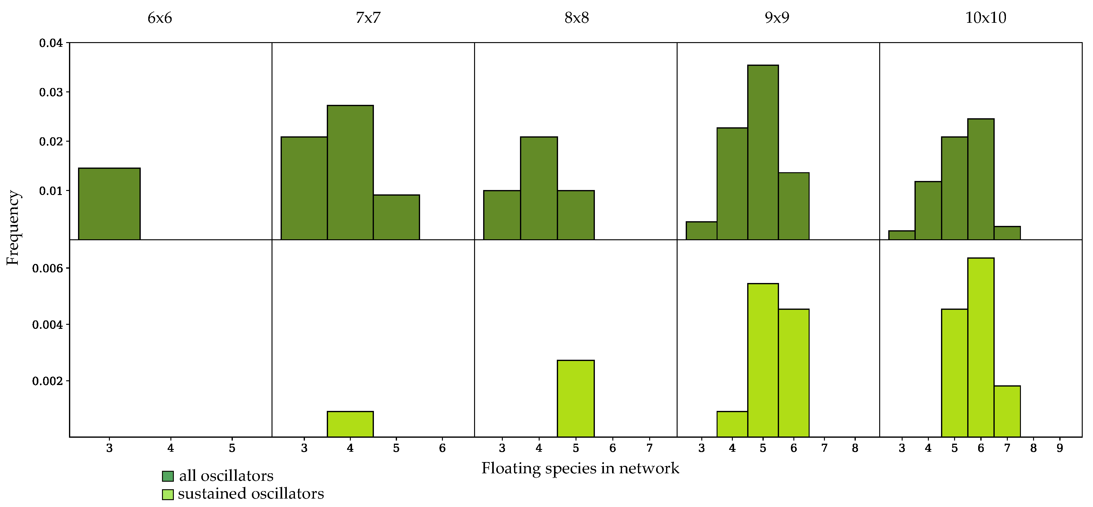
Figure 6.
Frequency of occurrence of oscillatory dynamics in randomly-generated networks with a 1:1.5, number of species to number of reactions ratio, binned by number of floating species in the network. (Top row) Frequency of oscillatory dynamics, including sustained and damped systems; (Bottom row) Frequency of sustained oscillatory dynamics.
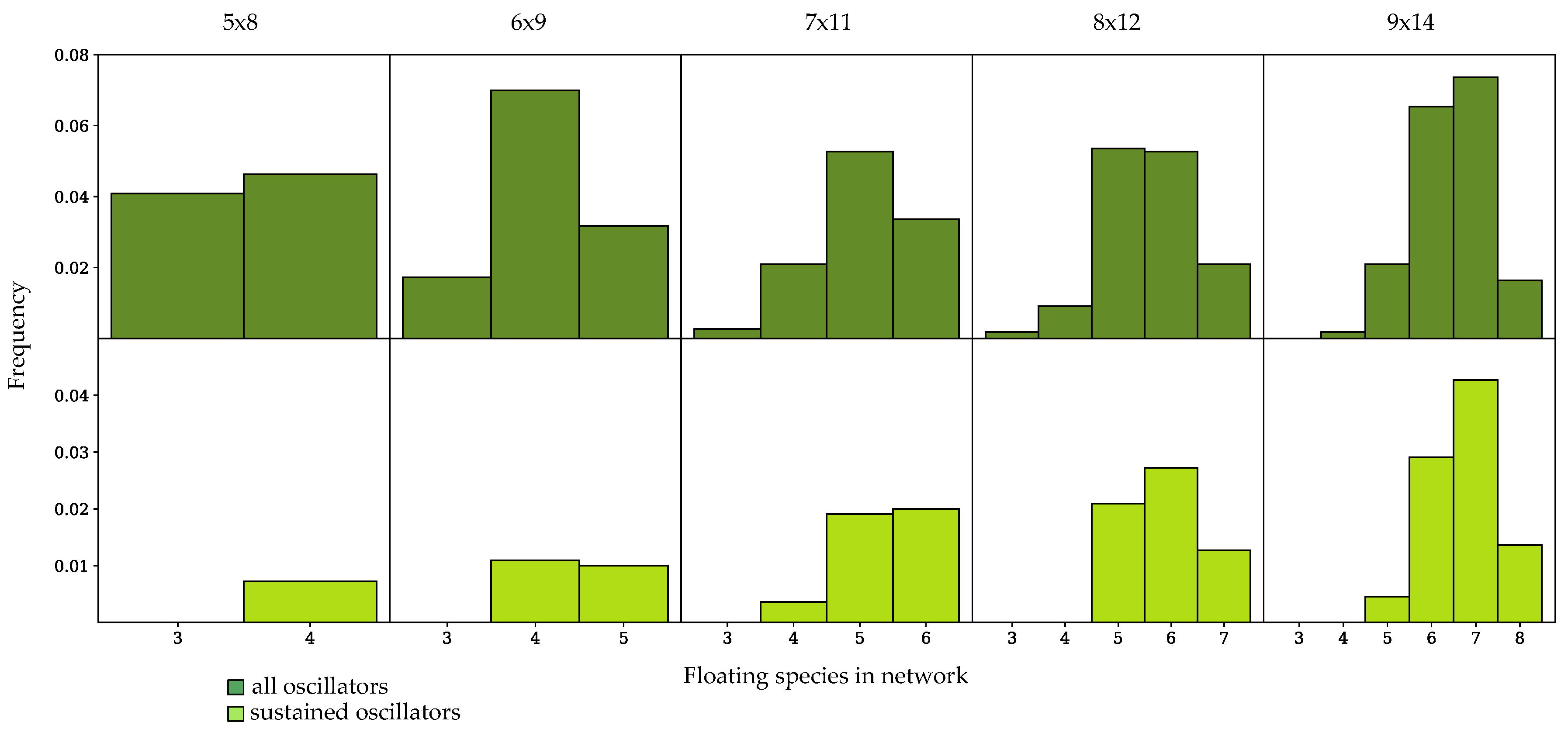
Figure 7.
Randomly-generated network with nine species and 10 reactions. Dark grey circles represent boundary nodes, and are replaced with constant production and decay rates in the reduced network. Green circles represent floating species. The network corresponds to Network 428 in the supplementary data of 10 × 10 networks allowing orphaned species. (a) complete network capable of oscillatory dynamics; (b) reduced network with essential species and reactions necessary for oscillation.
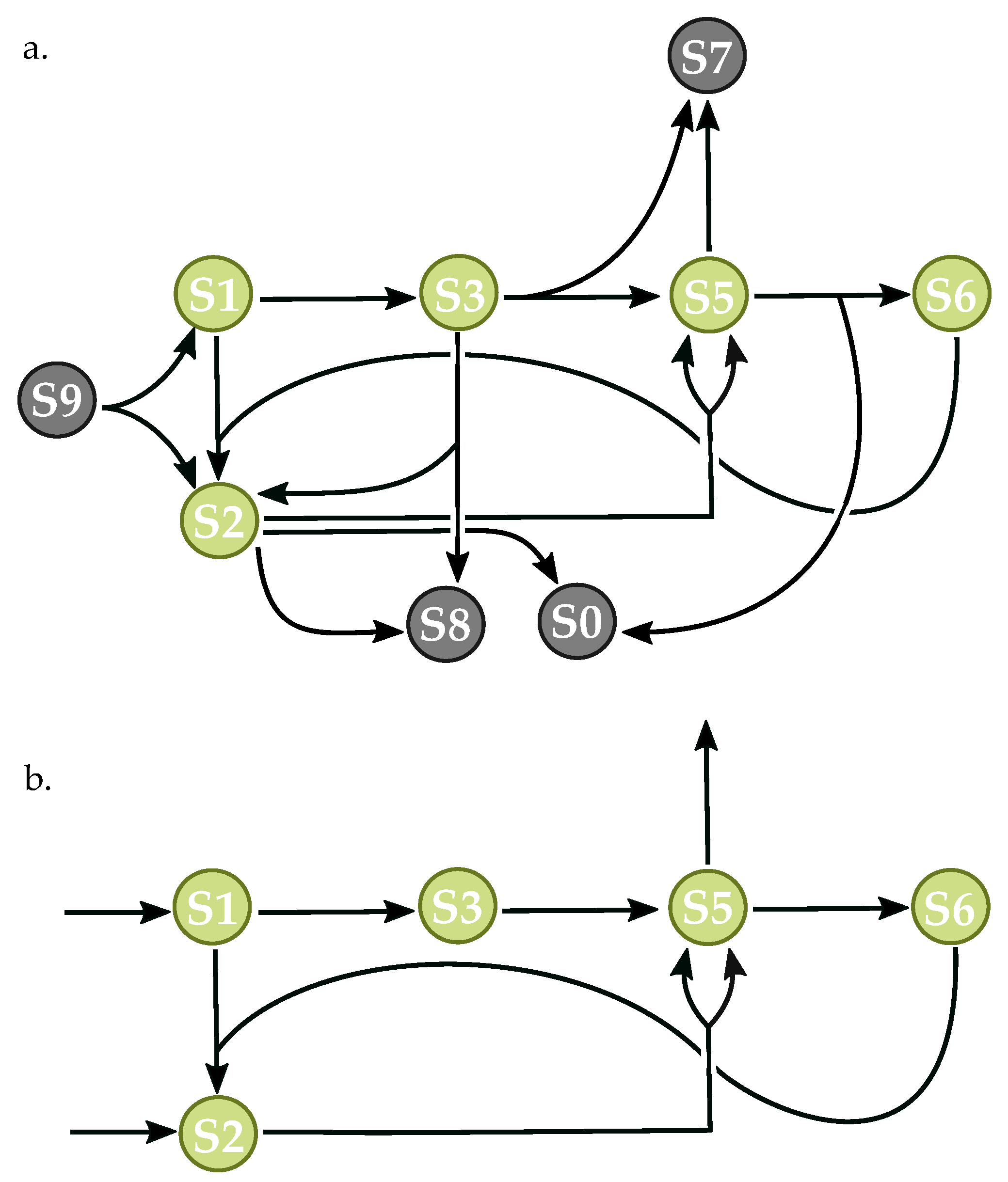
Figure 8.
Randomly-generated network with nine species and 10 reactions. The network corresponds to Network 7814 in the supplementary data of 10 × 10 networks allowing orphaned species. (a) complete network capable of oscillatory dynamics; (b) reduced network with essential species and reactions necessary for oscillation.

Table 1.
Test cases from the BioModels Database. Table model names and descriptions adapted from Chickarmane et al. with average runtime values generated by optimizing model parameter values for all test cases using the Pythonic bifurcation–evolution software [6].
Table 1.
Test cases from the BioModels Database. Table model names and descriptions adapted from Chickarmane et al. with average runtime values generated by optimizing model parameter values for all test cases using the Pythonic bifurcation–evolution software [6].
| Turning Point Model | Description | Runtime (s) |
|---|---|---|
| Tyson et al., 2003 (Figure 1e) [24] | Irreversible bistable switch | 9.10 |
| Tyson et al., 2003 (Figure 1f) [24] | Reversible bistable switch | 8.88 |
| Edelstein, 1970 [25] | Autocatalytic bistable switch | 17.70 |
| Hervagault and Canu, 1987 [22] | Bistable switch | 6.72 |
| Angeli et al., 2004 [26] | Bistable switch cdc2/wee1 | 8.16 |
| Oscillatory Model | Description | Runtime (s) |
| Tyson et al., 2003 (Figure 2a) [24] | Negative feedback oscillator | 1.24 |
| Tyson et al., 2003 (Figure 2b) [24] | Activator-inhibitor oscillator | 1.07 |
| Tyson et al., 2003 (Figure 2c) [24] | Substrate-depletion oscillator | 0.99 |
| Nicolis and Prigogine, 1977 [27] | Autocatalytic oscillator | 0.16 |
| Heinrich et al., 1977 [28] | Positive feedback oscillator | 0.16 |
| Seno et al., 1978 [23] | Modified Edelstein relaxation oscillator | 1.54 |
| Kholodenko, 2000 [29] | Mitogen-activated protein kinase feedback oscillator | 42.57 |
| Goldbeter, 1991 [30] | Mitotic oscillator | 1.20 |
| Francois et al., 2005 [31] | Mixed feedback loop oscillator | 6.18 |
| Lavrentovich and Hemkin, 2008 [32] | Spontaneous Ca oscillator | 1.70 |
Table 2.
Percentage of systems exhibiting sustained oscillatory dynamics in populations containing 1100 randomly-generated networks. Each population is defined by a characteristic network size, or number of species and reactions. Networks containing orphaned species were not included in these populations.
| Species | Reactions | Oscillators |
|---|---|---|
| 5 | 8 | 0.7% |
| 6 | 6 | 0.0% |
| 6 | 9 | 2.0% |
| 7 | 7 | 0.1% |
| 7 | 11 | 4.2% |
| 8 | 8 | 0.3% |
| 8 | 12 | 6.1% |
| 9 | 9 | 1.1% |
| 9 | 14 | 9.0% |
| 10 | 10 | 1.3% |
© 2019 by the authors. Licensee MDPI, Basel, Switzerland. This article is an open access article distributed under the terms and conditions of the Creative Commons Attribution (CC BY) license (http://creativecommons.org/licenses/by/4.0/).
Share and Cite
MDPI and ACS Style
Porubsky, V.L.; Sauro, H.M. Application of Parameter Optimization to Search for Oscillatory Mass-Action Networks Using Python. Processes 2019, 7, 163. https://doi.org/10.3390/pr7030163
AMA Style
Porubsky VL, Sauro HM. Application of Parameter Optimization to Search for Oscillatory Mass-Action Networks Using Python. Processes. 2019; 7(3):163. https://doi.org/10.3390/pr7030163
Chicago/Turabian StylePorubsky, Veronica L., and Herbert M. Sauro. 2019. "Application of Parameter Optimization to Search for Oscillatory Mass-Action Networks Using Python" Processes 7, no. 3: 163. https://doi.org/10.3390/pr7030163
Note that from the first issue of 2016, this journal uses article numbers instead of page numbers. See further details here.