Combined Estimation and Optimal Control of Batch Membrane Processes

Abstract

In this paper, we deal with the model-based time-optimal operation of a batch diafiltration process in the presence of membrane fouling. Membrane fouling poses one of the major problems in the field of membrane processes. We model the fouling behavior and estimate its parameters using various methods. Least-squares, least-squares with a moving horizon, recursive least-squares methods and the extended Kalman filter are applied and discussed for the estimation of the fouling behavior on-line during the process run. Model-based optimal non-linear control coupled with parameter estimation is applied in a simulation case study to show the benefits of the proposed approach.

1. Introduction

In the last few decades, an increased focus has been given to the membrane technology, which is used both in production and down-stream processing. Membrane technologies are exploited in a variety of processes, such as in membrane reactors, membrane distillation, diafiltration, dialysis, electrolysis, etc. All of these employ principles of membrane separation [1]. There are, however, certain limitations for the application. The major obstacle is the membrane fouling, which refers to the blockage of membrane pores during filtration, causing a decrease in the production rate. Although membrane fouling is an inevitable phenomenon occurring during the filtration process, it can be controlled and its influence alleviated [2].

There are several operational approaches to deal with membrane fouling. These mainly include scheduling of membrane cleaning cycles and on-line fouling control strategies [2]. These techniques usually require mathematical models for predicting the fouling behavior. The first attempt to describe the fouling behavior in a unified model was presented by Hermia [3] who developed four types of fouling behavior. Few works have then been devoted to model-based optimal control of membrane-assisted processes [4,5] and membrane fouling and cleaning [6,7]. However, optimal control requires knowledge of process model parameters. Thus, in the case of unknown parameters in the model, on-line parameter estimation may be performed in order to improve the process control performance. For this purpose, several methods can be applied, such as common least-squares or some more advanced methods. In Charfi et al. [8], an estimation of the fouling mechanism model proposed by Hermia was conducted for microfiltration and ultrafiltration in a membrane bioreactor using experimental data reported in the literature.

Parameter identifiability has to be addressed before the actual estimation step. If a model is non-identifiable, the estimated parameters will lead to errors in subsequent model predictions [9]. The identifiability test also provides a guideline for how to simplify the model structure or indicates when more measurements are needed to allow for unique identifiability [10].

Recently, the optimal control of a diafiltration process in the presence of fouling was proposed [11]. The obtained control law depends mainly on the parameters of membrane flux and fouling. In the subsequent work, an on-line control strategy was considered that incorporated parameter estimation using the extended Kalman filter (EKF) [12]. In this paper, we focus more broadly on the optimal operation of a diafiltration process under fouling where parameter estimation is used to determine the parameters of the fouling model. Compared to the work [12], in this paper, we provide a comparison of the estimation of the unknown parameters using several optimization-based (least-squares and moving-horizon estimation), as well as recursive (recursive least-squares estimation and extended Kalman filter) methods by considering also measurement and process noise, and we assess their performance on the highly non-linear estimation problem that arises from the nature of the employed process model. In addition, the identifiability test is also performed in order to reveal whether the model parameters can be estimated based on available measurements.

The paper is organized as follows. In the next section, the general formulation of a batch diafiltration process is introduced. In Section 3, we provide a detailed analysis of the membrane fouling phenomena, and we also discuss the modeling of the membrane fouling. Section 4 provides the definition of the problem of the optimal operation of the diafiltration process. In Section 5, a review of identifiability detection methods is given with the main focus on non-linear models described by ordinary differential equations (ODEs). The results and implications of the performed identifiability tests are presented. An introduction is then given to the considered parameter estimation problem, and four different estimation methods are briefly presented. Finally, a simulation study is provided in Section 6 with a detailed discussion and analysis of the obtained results.

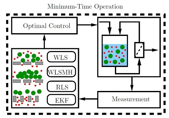
2. Process Description

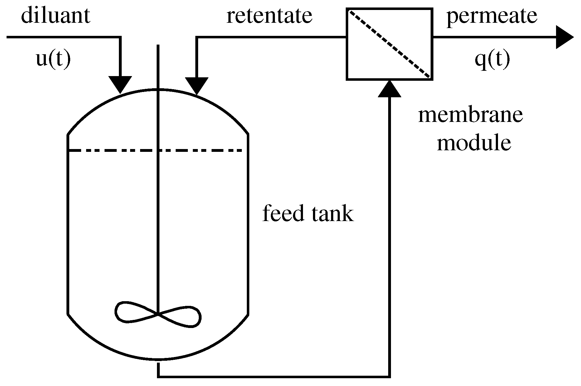
In this paper, we consider the batch diafiltration process shown in Figure 1. The batch process operates under constant pressure and temperature. The overall batch process consists of a feed tank and a membrane module. We consider that the process solution consist of a solvent (water), macro-solute (high molecular weight component) and micro-solute (low molecular weight component). The process solution is brought from the feed tank to the membrane by means of mechanical energy (e.g., pump). The membrane is designed to retain the macro-solute, while the micro-solute can easily pass through the membrane pores. The stream rejected by the membrane is called the retentate and is taken back into the feed tank. The stream that leaves the system is called the permeate, and its flow-rate is defined as $q=AJ$, where A is the membrane area and J is the permeate flux per unit area of the membrane. The flow rate of the permeate stream is a function of both concentrations of the individual solutes and of time, in the case of the occurrence of fouling phenomena.

The control of the batch diafiltration process can be achieved by adjusting the flow-rate of the solvent (diluent) into the feed tank. Then, the control variable α is defined as the ratio between the inflow into the feed tank and the outflow from the membrane module. Traditional approaches to the operation of the diafiltration process consider sequences of operating regimes, which differ in the rate of diluent addition:

• Concentration mode: During this mode, no diluent is added into the feed tank, i.e., $\alpha =0$.
• Constant-volume diafiltration mode: Here, the rate of inflow of the diluent is kept the same as the rate of permeate outflow, i.e., $\alpha =1$.
• (Pure) Dilution mode: In this mode, a certain amount of diluent can be added instantaneously into the feed tank. This can be represented as $\alpha \to \infty$.

Regarding the practical applicability of the pure dilution mode, as will be shown further, the optimal operation would involve the pure dilution mode as an initial or a final step. In both of these cases, the pure dilution step can be performed out of the batch as a pre-/post-treatment of the separated solution.

The process model [13] is constituted by the solutes mass balance equations, which have the following form:

$$\frac{\mathrm{d}{c}_i}{\mathrm{d}t}=\frac{c_{i}q}{V}(R_i-\alpha ),c_i\left(0\right)=c_{i,0},i=1,2,$$

(1)

where V is the volume in the feed tank and $c_i$ denotes the concentration of the i-th solute; $i=1$ for macro-solute; and $i=2$ for micro-solute. $R_i$ is the observed rejection coefficient of the i-th solute, which describes the ability of the membrane to retain the solute. The total mass balance is defined as follows:

$$\frac{\mathrm{d}V}{\mathrm{d}t}=\alpha q-q=(\alpha -1)AJ,V\left(0\right)=V_0,$$

(2)

where $V_0$ is the initial volume of the process solution.

In many cases, the rejection coefficient $R_i$ is a function of concentrations. In this paper, we will consider that the rejections are ideal, given and constant for both solutes ($R_1=1$ and $R_2=0$). This means that the membrane is perfectly impermeable to macro-solute and that only the micro-solute can pass through the membrane. Moreover, since only the micro-solute can pass through the membrane, the mass of macro-solute in the system will not change and remains constant, such that $c_1\left(t\right)V\left(t\right)=c_{1,0}{V}_0$. Based on these assumptions, we can eliminate the differential equation for the volume (2), and the model has now the following form:

$$\begin{array}{cc}\hfill \frac{\mathrm{d}{c}_1}{\mathrm{d}t}& =c_1^2\frac{AJ}{c_{1,0}{V}_0}(1-\alpha ),c_1\left(0\right)=c_{1,0},\hfill \end{array}$$

(3)

$$\begin{array}{cc}\hfill \frac{\mathrm{d}{c}_2}{\mathrm{d}t}& =-c_1{c}_2\frac{AJ}{c_{1,0}{V}_0}\alpha ,c_2\left(0\right)=c_{2,0}.\hfill \end{array}$$

(4)

3. Membrane Fouling

One of the major obstacles in the field of membrane-assisted processing is the membrane fouling. The membrane fouling is caused by the deposit of the solutes in/on the membrane pores. The main consequence of the membrane fouling is the decrease in the permeate outflow due to the blockage of the pores. The most important factors that cause the membrane fouling are the feed properties and membrane material. Moreover, membrane fouling can increase when the concentration polarization effect takes place. In [14], the authors have shown that during the membrane filtration, the retained macro-solute can form a gel layer over the membrane surface. The formation of such a gel layer can increase the interactions between the solutes and the membrane surface, which eventually lead to membrane fouling. Further, the process variables, such as temperature and pressure, may also contribute to membrane fouling [15].

As mentioned above, the main consequence of the membrane fouling is the decrease in the permeate flow rate, which results in the increase of the overall processing time. If the membrane becomes heavily fouled, cleaning must be performed. In some cases, even replacement of the membrane module must be carried out, which leads to the increase of the production costs.

In the past three decades, the modeling of membrane fouling became very important. In 1982, Hermia [3] derived a unified fouling model for dead-end filtration in terms of total permeate flux and time, which has the following form:

$${\displaystyle \frac{{\mathrm{d}}^{2}t}{\mathrm{d}{V}_{\mathrm{p}}^2}}=K{\left({\displaystyle \frac{\mathrm{d}t}{\mathrm{d}{V}_{\mathrm{p}}}}\right)}^n,$$

(5)

where $V_{\mathrm{p}}$ is the permeate volume, t is time and K represents the fouling rate constant. From the above unified fouling model, four classical fouling models can be derived for different values of the fouling parameter n. The four models are cake filtration ($n=0$), intermediate blocking ($n=1$), internal blocking ($n=3/2$) and the complete blocking model ($n=2$). By integration of (5), we obtain the differential equation for the permeate flux [16,17], which is expressed as:

$$\begin{array}{c}\hfill {\displaystyle \frac{\mathrm{d}J}{\mathrm{d}t}}=-K{A}^{2-n}{J}^{3-n}.\end{array}$$

(6)

This equation can be solved to give an explicit solution $J(t,K,n,A,J_0)$ if the parameters A, K and n are constant and $J_0$ is the initial flux at time $t=0$. However, this model holds only for dead-end filtration mode. In order to account for the dynamics of the cross-flow system, which is considered in this paper, we propose to substitute the initial flux $J_0(t=0)$ with the flux of an unfouled membrane $J_0(c_1,c_2)$.

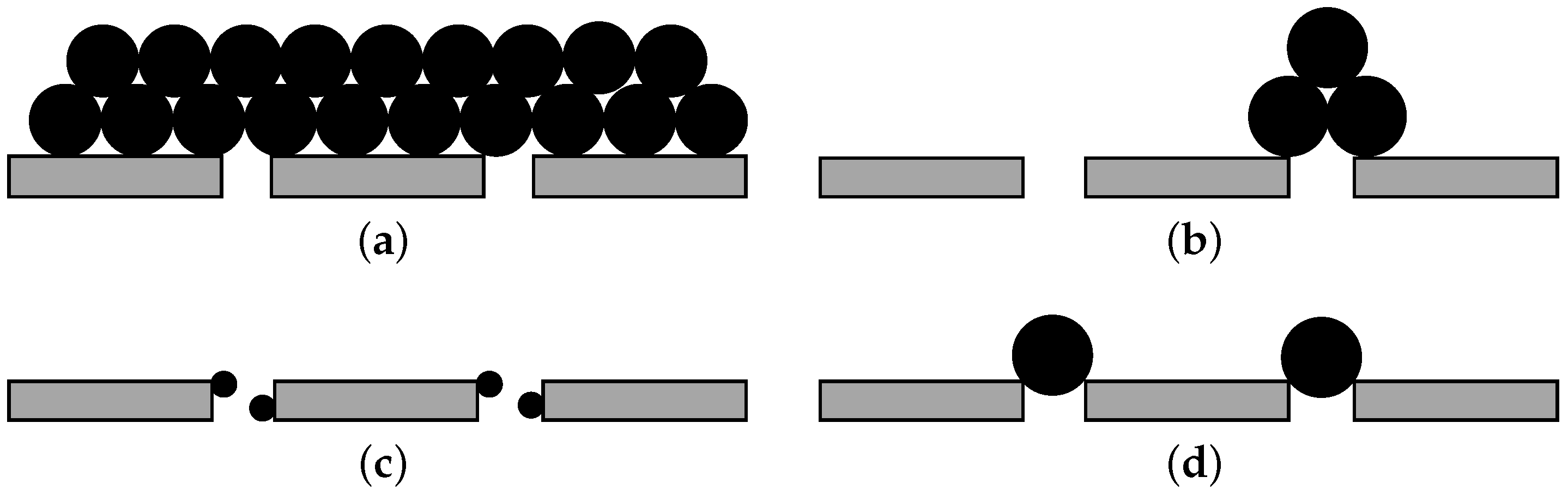
In Figure 2, we show the graphical representation of the four standard fouling models. The models differ in the way that the solutes deposit on/in the membrane surface. In the following subsections, we will briefly discuss the individual fouling models.

3.1. Cake Filtration Model

The cake filtration model considers that the solutes brought to the membrane surface will form a multi-layered cake formation shown in Figure 2a. The multi-layered formation is caused by the repeating deposit of the solutes on the membrane surface. The parameter n is set to zero, and the permeate flux has the following form:

$$\frac{1}{J^2}=\frac{1}{J_0^2}+2K{A}^{2}t.$$

(7)

where J in ${\mathrm{m}}^3/\mathrm{s}/{\mathrm{m}}^2$ is the permeate flow per unit area of the membrane and $J_0$ is the flux of an unfouled membrane.

3.2. Intermediate Blocking Model

The intermediate fouling model also considers that the solute will block all of the pores. However, in this case, the solutes can also deposit on each other, as illustrated in Figure 2b. To derive the model, the parameter n is equal to one, and the permeate flux is of the form:

$$\frac{1}{J}=\frac{1}{J_0}+KAt.$$

(8)

3.3. Internal Blocking Model

The aforementioned fouling models do not consider the fouling to take place inside the membrane pores. This is not the case with an internal blocking model (Figure 2c). This type of fouling results in the decrease of the diameter of the membrane pores, which leads to the decrease of the permeate flow. For the internal blocking model, the parameter n is equal to 3/2, and the permeate flux is derived as:

$$\frac{1}{\sqrt{J}}=\frac{1}{\sqrt{J_0}}+{\displaystyle \frac{1}{2}}K{A}^{1/2}t.$$

(9)

3.4. Complete Pore Blocking Model

The complete pore blocking model considers that all of the solutes brought to the membrane surface will block the membrane pores (Figure 2d). Therefore, the permeate flow will be reduced. Moreover, the blockage of the pores is caused only if the molecules of the solutes are larger than the membrane pores. The complete blocking model can be derived from (5) if $n=2$ and is of the following form:

$$lnJ=ln{J}_0-Kt,$$

(10)

Note that unlike in the previous cases, the permeate flux does not depend on the membrane area.

4. Optimization Problem

The main operational objective of the diafiltration plant is to process as much solution as possible. This can only be achieved by pursuing the time-optimal batch recipes with tight scheduling. Consequently, as scheduling is here usually a rather trivial task, we concentrate on the time-optimal control problem of a batch membrane process in the presence of membrane fouling.

4.1. Problem Definition

The objective is to identify such a time-dependent function $\alpha \left(t\right)$ that will drive the system from the initial concentrations to the required final concentrations in the minimum time. The optimization problem reads as:

$$\begin{array}{cc}\hfill {\mathcal{J}}^{*}& =\underset{\alpha \left(t\right)}{min}{\int }_0^{t_{\mathrm{f}}}1\mathrm{d}t,\hfill \end{array}$$

(11)

$$\begin{array}{cc}\hfill s.t.{\dot{c}}_1& =\frac{c_1^{2}AJ}{c_{1,0}{V}_0}(1-\alpha ),c_1\left(0\right)=c_{1,0},c_1\left(t_{\mathrm{f}}\right)=c_{1,\mathrm{f}},\hfill \end{array}$$

(12)

$$\begin{array}{cc}\hfill {\dot{c}}_2& =-\frac{c_1{c}_{2}AJ}{c_{1,0}{V}_0}\alpha ,c_2\left(0\right)=c_{2,0},c_2\left(t_{\mathrm{f}}\right)=c_{2,\mathrm{f}},\hfill \end{array}$$

(13)

$$\begin{array}{cc}\hfill J& =J(t,J_0(c_1,c_2),K,n),\hfill \end{array}$$

(14)

$$\begin{array}{cc}\hfill \alpha & \in [0,\infty ).\hfill \end{array}$$

(15)

We assume that this optimization problem is feasible, i.e., the process design ensures that the final conditions can be met within admissible input trajectories. This optimization problem can be approximately solved using various numerical methods [18] of dynamic optimization (e.g., control vector parametrization or complete discretization). However, an analytical solution is available. This was shown in [19] and is briefly reviewed in the following.

4.2. Nominal Optimal Operation

In our recent study [19], we derived analytically the complete optimal operation for a diafiltration process in the presence of membrane fouling using Pontryagin’s minimum principle [20,21]. The optimal operation is an explicit non-linear control strategy defined on three time intervals as follows:

• In the first interval, the control is kept on the boundaries (e.g., minimum or maximum) until the singular curve is reached:

  $$\begin{array}{c}\hfill S(t,c_1,c_2,K,n)=J+c_1{\displaystyle \frac{\partial J}{\partial c_1}}+c_2{\displaystyle \frac{\partial J}{\partial c_2}}=0.\end{array}$$

  (16)
  The minimum control action ($\alpha =0$) is applied if the initial concentrations lie to the left side of the singular surface ($S(0,c_{1,0},c_{2,0},K,n)<0$) in the state diagram. Conversely, the maximum ($\alpha \to \infty$) control action is applied when the initial concentrations are on the right of the singular curve ($S(0,c_{1,0},c_{2,0},K,n)>0$).
• Once the singular curve is reached, the singular control is applied, which forces the states to stay on the singular curve:

  $$\begin{array}{c}\hfill \alpha (t,c_1,c_2,K,n)={\displaystyle \frac{{\displaystyle \frac{\partial S}{\partial c_1}}{c}_1}{{\displaystyle \frac{\partial S}{\partial c_1}}{c}_1+{\displaystyle \frac{\partial S}{\partial c_2}}{c}_2}}+{\displaystyle \frac{{\displaystyle \frac{\partial S}{\partial t}}}{{\displaystyle \frac{c_{1}AJ}{c_{10}{V}_0}}\left({\displaystyle \frac{\partial S}{\partial c_1}}{c}_1+{\displaystyle \frac{\partial S}{\partial c_2}}{c}_2\right)}}.\end{array}$$

  (17)
  This step is terminated once the ratio of the concentrations is equal to the ratio of the final concentrations or once the final concentration of the micro-solute is reached.
• In the last step, the control is kept on one of the boundaries similar to the first step with the difference that the operation mode to be applied is determined by the final time constraints. The concentration mode ($\alpha =0$) is applied if the final concentration of the micro-solute has been reached. The dilution mode with $\alpha \to \infty$ is applied once the ratio of the final concentrations is equal to the final one. Both steps are performed until the final concentrations are reached.

For a particular case of initial and final concentrations, any of the three steps can be missing. For instance, if initial (respectively final) concentrations lie on the singular case, then the first (respectively last) step will be skipped. Another case would occur if the singular case cannot be reached before the control has to switch from the first to the last step, so the optimal operation will consist entirely of saturated control arcs.

4.3. Optimal Operation with Imperfect Knowledge of Fouling Model Parameters

It can be easily shown that the optimal control structure does not depend on the unknown fouling parameters in the first and last step of the optimal operation. This comes from the fact that, on the one hand, the initial flux is not influenced by the fouling, as $J\left(0\right)=J_0$, and on the other hand, the last step is determined by the active constraints, which are independent of the fouling behavior.

These observations imply that one can distinguish two cases in the on-line optimal operation under imperfect knowledge of the fouling model:

• If the operation starts with the concentration mode, the a priori knowledge of unknown parameters K and n should be improved during this step by parameter estimation, such that the switching time can be determined accurately. If this estimation is successful, the optimal singular surface is followed thereafter.
• Should the optimal operation commence with a pure dilution step, the entry point to the singular surface would be known exactly, as it only depends on $J_0$. In other words, the amount of the diluent that should be added at the beginning of the operation does not depend on the parameters of the fouling model. It would then be again necessary to improve the knowledge about the unknown parameters in order to maintain the singular-surface condition.

Clearly, the on-line parameter estimation will yield adequate results only if (a) a sufficient amount of data can be gathered and if (b) significant sensitivity is present between measured outputs and estimated parameters on the particular arc of the optimal solution. The first condition requires that the optimal concentration mode, respectively singular arc, lasts sufficiently long, which will likely result in the negligible suboptimality of the on-line control strategy. The latter condition suggests the provision of the persistence of excitation in the system. This might be critical should the parameter estimation be required to yield accurate parameter estimates when the system resides on the singular arc. For example, if the optimal singular flux is constant, then the set of obtained flux measurements will not bring enough new information about the fouling behavior. This case will further be addressed in Section 6 where the interesting question is to find out what the trade-off is between the insensitivity of the objective function to the control on the singular arc and the inaccuracy of parameter estimates.

5. Parameter Estimation Problem

In this section, we will discuss parameter identifiability and parameter estimation techniques. Several studies have employed standard estimation methods to obtain the fouling parameters necessary for the control of membrane processes. In [8], the authors have proposed to employ the least-squares method to identify the fouling rate constant (K) for the standard fouling models. However, this procedure was performed completely off-line with the necessity of initial probing runs to obtain the experimental measurements of flux based on which the fouling rate constant could be determined. Moreover, only the fouling rate constant was estimated with a fixed type of fouling model. Since the derived optimal control depends also on the information of the type of fouling model, the estimation of both the unknown fouling parameters ($K,n$) is followed in this work. Furthermore the estimation is performed on-line, which eliminates the necessity of any initial experiments.

The on-line estimation is coupled with the aforementioned optimal feedback control law, which is updated iteratively with the estimated values of the parameters of the fouling model. In our recent paper [12], we have introduced this strategy using EKF. In this paper, we provide an assessment of the performance of some other commonly-used model-based estimators.

5.1. Problem Definition

We will consider that the process dynamics is described by a set of ODEs with initial conditions and expressed in the following form:

$$\begin{array}{cccc}\hfill {\dot{c}}_1& =\frac{c_1^{2}AJ}{c_{1,0}{V}_0}(1-\alpha ),\hfill & \hfill c_1\left(0\right)& =c_{1,0},\hfill \end{array}$$

(18)

$$\begin{array}{cccc}\hfill {\dot{c}}_2& =-\frac{c_1{c}_{2}AJ}{c_{1,0}{V}_0}\alpha ,\hfill & \hfill c_2\left(0\right)& =c_{2,0},\hfill \end{array}$$

(19)

$$\begin{array}{cccc}\hfill \dot{\tau }& =1,\hfill & \hfill \tau \left(0\right)& =0,\hfill \end{array}$$

(20)

where τ replaces the explicit appearance of time with a new state, and the permeate flux J is defined as follows:

$$J(\tau ,J_0(c_1,c_2),n,K,A)=J_0{\left(1+K(2-n){\left(A{J}_0\right)}^{2-n}\tau \right)}^{\left(1/(n-2)\right)},$$

(21)

We will rewrite the above differential equations into the following compact form:

$$\begin{array}{c}\hfill {\displaystyle \dot{\mathit{x}}}={\displaystyle \mathit{f}}({\displaystyle \mathit{x}},{\displaystyle \mathbf{\theta }},{\displaystyle \mathit{u}}),\end{array}$$

(22)

where $\mathit{x}={(c_1,c_2,\tau )}^T$ is the vector of state variables, $\mathbf{\theta }={(K,n)}^T$ is the vector of estimated parameters and $\mathit{u}$ is the control action. For the estimation of the unknown parameters, we assume that the concentrations of the individual solutes ($c_1,c_2$) and also the permeate flux (J) can be measured.

5.2. Identifiability Problem

The problem of the parameter identifiability of dynamic models is a special case of the observability problem. It is often the case that the parameters of a model have unknown values. These values can be estimated from observing the input-output behavior.

Before the model parameters can be estimated, the identifiability analysis must be performed. The property of identifiability is the ability to deduce the values of the model parameters uniquely in terms of known quantities based on input and output variables and their time derivatives. In order to investigate identifiability of (18) to (20), we will first introduce a definition of identifiability.

Definition 1. 

A dynamic system described by (22) and (25) is identifiable if the parameter vector $\mathbf{\theta }$ can uniquely be determined from the given system input $\mathit{u}$ and the measurable system output $\mathit{y}$. If no solution can be found for the given vector of unknown parameters $\mathbf{\theta }$, then the model is non-identifiable.

The identifiability analysis also distinguishes whether the parameter vector can uniquely be identified or not. In this regard, a system is said to be structurally globally identifiable if for any admissible input and any two parameter vectors ${\mathbf{\theta }}_1$ and ${\mathbf{\theta }}_2$, $\mathit{y}(\mathit{u},{\mathbf{\theta }}_1)=\mathit{y}(\mathit{u},{\mathbf{\theta }}_2)$ holds if and only if ${\mathbf{\theta }}_1={\mathbf{\theta }}_2$. A system is said to be structurally locally identifiable if for any parameter vector $\mathbf{\theta }$ within an open neighborhood of some point, $\mathit{y}(\mathit{u},{\mathbf{\theta }}_1)=\mathit{y}(\mathit{u},{\mathbf{\theta }}_2)$ holds if and only if ${\mathbf{\theta }}_1={\mathbf{\theta }}_2$.

There are many well-established methods for determining the identifiability of linear systems. However, fewer methods are applicable for non-linear systems. The most common methods for the identifiability test include: the direct test [22], the identifiability of the corresponding linearized system [22], the similarity transformation method [23,24], power series expansion [25], the generating series approach [26] and differential algebra [27]. Two of these methods are used for the identifiability analysis in this work.

5.2.1. Identifiability of the Corresponding Linearized System

Local linearization of the non-linear models can be considered for the identifiability test. However, the identifiability of the linearized model is only a necessary condition [22].

There are several methods for the identifiability of linear systems. One method is to consider parameters as dummy state variables with time derivatives equal to zero. The observability rank test can then be applied where the observability matrix O of a linear system $\dot{\mathit{x}}=\mathit{A}\left(\mathbf{\theta }\right)\mathit{x}+\mathit{B}\left(\mathbf{\theta }\right)\mathit{u},\mathit{y}=\mathit{C}\left(\mathbf{\theta }\right)\mathit{x}$,

$$\begin{array}{c}\hfill O={\left[\begin{array}{c}{\displaystyle \mathit{C}}{\displaystyle \mathit{C}}{\displaystyle \mathit{A}}\cdots {\displaystyle \mathit{C}}{{\displaystyle \mathit{A}}}^{n-1}\end{array}\right]}^T,\end{array}$$

(23)

should be of full rank n, where n is the dimension of the vector of state variables. Rigorously speaking, this approach can only serve to detect the non-identifiability of the parameters.

5.2.2. Generating Series Approach

This approach is based on the computation of Lie derivatives, which allows one to expand the output variables with respect to input variables. By computing Lie derivatives, a set of resulting coefficients is formed, which is then used to compute the parametric solution. Based on this solution, the identifiability of the model is checked. A drawback of this method is that the sufficient number of Lie derivatives to be considered is unknown. In order to easily visualize the structural identifiability problem and to assist in the solution, identifiability tableau is proposed [26]. This tableau expresses the dependency between parameters by using the Jacobian matrix of exhaustive summary, i.e., a set of relations that depends only on the parameters. The tableau is represented by a “$0-1$” matrix, which represents whether there is a dependency between Lie derivatives and the parameters “1”, or not “0”. The identifiability is then checked by examining whether there is a unique “1” in a row of the tableau. If so, then there exists a unique dependency between the Lie derivative and a parameter. Thus, the corresponding parameter is structurally identifiable [9,28].

5.3. Software Tools for the Identifiability Test

There are few frameworks and software tools available that assist in identifiability analysis [29,30]. To the authors knowledge, there are three common software tools that use one of the above-mentioned methods for testing global identifiability of non-linear systems. These are DAISY [31], COMBOS [30] and GenSSI. The open-source tool GenSSI implements the generating series approach and is chosen here for the identifiability analysis of the parameters. This is due to the model structure, which must be strictly polynomial in order to be implemented in DAISY and in COMBOS. In our case, the model of the diafiltration process with fouling does not satisfy this requirement.

GenSSI module is written in MATLAB and can be used for any general linear, non-linear ODE or differential algebraic system. To run the identifiability test, the user needs to specify the model equations, input and output variables, initial conditions, parameters to be identified and the number of Lie derivatives. In the case of the detection of non-identifiability, GenSSI also provides information on individual parameters and their global or local identifiability. This information can guide the proper reformulation of the model [9,28].

Results and Discussion

The identifiability problem was solved for the membrane fouling process described by (3) and (4) using both the observability matrix test and generating series approach. The results showed that the parameters $K,n$ in the membrane fouling model are not observable with the vector of measurement $\mathit{y}={(c_1,c_2,J)}^T$. This is due to the fact that parameters enter the process equations via J only, and therefore, there are infinitely many combinations that can lead to actual J. Therefore, a new measurement must be added, which is a different function of the estimated parameters. For this reason, the time derivative of the flux $\dot{J}$ is considered as a new measurement. Based on the results given by GenSSI, the augmented model of membrane fouling, which also considers the time-derivative of the flux as a measured variable, is globally identifiable. This means that the two parameters $K,n$ can be identified based on the measured variables from any given initial conditions. The identifiability of the parameters was also confirmed by using the observability matrix.

It is usually not possible to measure the derivative of the flux directly. Therefore, an approximation of the third order is considered, which reads as:

$$\begin{array}{c}\hfill \frac{\mathrm{d}J}{\mathrm{d}t}\approx \frac{J_{k-3}-6J_{k-2}+3J_{k-1}+2J_k}{6T_s}.\end{array}$$

(24)

where $T_s$ represents the sampling time. Different approximations were tested; the third order is a good compromise between accuracy and complexity.

Then, the considered measured outputs in discrete-time samples (k) are as follows:

$$\begin{array}{c}\hfill {{\displaystyle \mathit{y}}}_k={\displaystyle \mathit{h}}({{\displaystyle \mathit{x}}}_k,{\displaystyle \mathbf{\theta }})={(c_1,c_2,J,\dot{J})}^T.\end{array}$$

(25)

This form of output equation is further considered for parameter estimation.

5.4. Parameter Estimation Methods

Different parameter estimation methods are discussed in the following subsections. They mainly differ in the consideration of the parameter estimation problem as non-linear (least-square method), mildly non-linear (least-squares method with moving horizon) or almost linear (recursive least-squares method and EKF). Note that this consideration implies whether the non-linear programming problem (NLP) needs to be solved with each newly-gathered measurement or whether a recursive approach is sufficient, where only a few mathematical operation (e.g., matrix-vector multiplications) are performed. Here, a critical point is presented by the tendency of the recursive methods to rapidly diverge should the process (and its model) exhibit strong non-linear behavior.

5.4.1. Weighted Least-Squares Method

One of the most used methods for parameter estimation is the weighted least-squares (WLS) method. Compared to the standard least-squares method, the WLS method considers that different measured outputs can contribute differently to the estimation of unknown parameters based on their variability and statistical significance [32]. For the on-line parameter estimation, it must be, however, considered that with each new measurement, a new NLP problem must be solved, and moreover, if a large set of experimental points is available, numerical problems can occur due to the gradually increasing complexity of the optimization problem. The optimization problem that needs to be solved in each sampling time is as follows:

$$\begin{array}{cc}\hfill {{\displaystyle \widehat{\mathbf{\theta }}}}_k=& arg\underset{\mathbf{\theta }}{min}\sum _{j=0}^k{({{\displaystyle \mathit{y}}}_j-{{\displaystyle \widehat{\mathit{y}}}}_j)}^T{{\displaystyle \mathit{R}}}^{-1}({{\displaystyle \mathit{y}}}_j-{{\displaystyle \widehat{\mathit{y}}}}_j)\hfill \end{array}$$

(26)

$$\begin{array}{cc}& \mathrm{s}.\mathrm{t}.\left(18\right)\mathrm{to}\left(20\right),\hfill \end{array}$$

(27)

$$\begin{array}{cc}& {{\displaystyle \widehat{\mathit{y}}}}_j={\displaystyle \mathit{h}}({{\displaystyle \mathit{x}}}_j,{\displaystyle \mathbf{\theta }}),\hfill \end{array}$$

(28)

$$\begin{array}{cc}& {{\displaystyle \mathbf{\theta }}}_{\min }\le {\displaystyle \mathbf{\theta }}\le {{\displaystyle \mathbf{\theta }}}_{\max },\hfill \end{array}$$

(29)

where $\mathit{y}$ represents the vector of obtained measurements, $\mathit{R}$ is the covariance matrix for the measurement noise and ${\mathbf{\theta }}_{\min }$, ${\mathbf{\theta }}_{\max }$ are the minimum and maximum values of the parameters, respectively.

5.4.2. Weighted Least-Squares Method with Moving Horizon

The weighted least-squares method with moving horizon [33] is very similar to the previously-discussed method. However, in this case, not the whole measurement set is considered, but only recent measurements on a constant moving horizon (MH) contribute actively to the estimation. The influence of the past measurements, gathered prior to the moving horizon, is not neglected, but rather considered through the parametric covariance matrix P as a priori knowledge of the parameters, similarly to Bayesian estimation. The covariance matrix then penalizes a drift of the new estimates from their a priori values in the objective function [34]. In [35], it has also been shown that the moving-horizon estimation is equivalent to the extended Kalman filter if the first-order approximation of dynamics and no constraints are considered. A distinct advantage of this method is that since a fixed-length horizon of measured outputs is considered, the NLP problem that needs to be solved, when new measurements are gathered, is of approximately fixed complexity and might be easier to solve than the optimization problem in WLS estimation. The resulting non-linear problem reads as:

$$\begin{array}{cc}\hfill {{\displaystyle \widehat{\mathbf{\theta }}}}_k=& arg\underset{\mathbf{\theta }}{min}{({\displaystyle \mathbf{\theta }}-{{\displaystyle \widehat{\mathbf{\theta }}}}_{k-MH})}^T{{\displaystyle \mathit{P}}}_{k-MH}^{-1}({\displaystyle \mathbf{\theta }}-{{\displaystyle \widehat{\mathbf{\theta }}}}_{k-MH})+\sum _{j=k-MH}^k{({{\displaystyle \mathit{y}}}_j-{{\displaystyle \widehat{\mathit{y}}}}_j)}^T{{\displaystyle \mathit{R}}}^{-1}({{\displaystyle \mathit{y}}}_j-{{\displaystyle \widehat{\mathit{y}}}}_j)\hfill \end{array}$$

(30)

$$\begin{array}{cc}& \mathrm{s}.\mathrm{t}.\left(18\right)\mathrm{to}\left(20\right),\hfill \end{array}$$

(31)

$$\begin{array}{cc}& {{\displaystyle \widehat{\mathit{y}}}}_j={\displaystyle \mathit{h}}({{\displaystyle \mathit{x}}}_j,{\displaystyle \mathbf{\theta }}),\hfill \end{array}$$

(32)

$$\begin{array}{cc}& {{\displaystyle \mathbf{\theta }}}_{\min }\le {\displaystyle \mathbf{\theta }}\le {{\displaystyle \mathbf{\theta }}}_{\max }.\hfill \end{array}$$

(33)

It is worth mentioning that the matrix $\mathit{P}$ can be either selected as a constant matrix or one can apply the extended Kalman filter method to update the matrix $\mathit{P}$ in each sampling time to improve the convergence.

5.4.3. Recursive Least-Squares Method

The recursive least-squares method (RLS) iteratively finds parameter estimates that minimize the linearized least-squares objective function [36]. The parameter estimates are calculated at each sampling time based on the a priori knowledge of the parameters (through parametric covariance matrix) and the current measured outputs. The advantage of the method is that during the estimation, no NLP problem has to be solved. On the other hand, RLS does not explicitly consider the constraints on the estimated parameters in the updates of the covariance matrix, and thus, the a priori knowledge of parameters might be biased.

In order to apply the RLS method, we consider a Taylor expansion of the output function (25) to the first order:

$$\begin{array}{cc}\hfill {{\displaystyle \widehat{\mathit{y}}}}_k={\displaystyle \mathit{h}}({{\displaystyle \mathit{x}}}_k,{\displaystyle \mathbf{\theta }})& \approx {\displaystyle \mathit{h}}({{\displaystyle \mathit{x}}}_k,{{\displaystyle \widehat{\mathbf{\theta }}}}_{k-1})+{\left({\displaystyle \frac{\partial \mathit{h}({\mathit{x}}_k,\mathbf{\theta })}{\partial {\mathit{x}}_k}}{|}_{{\widehat{\mathbf{\theta }}}_{k-1}}{\displaystyle \frac{\partial x}{\partial \mathbf{\theta }}}{|}_{{\widehat{\mathbf{\theta }}}_{k-1}}+{\displaystyle \frac{\partial \mathit{h}({\mathit{x}}_k,\mathbf{\theta })}{\partial \mathbf{\theta }}}{|}_{{\widehat{\mathbf{\theta }}}_{k-1}}\right)}^T({{\displaystyle \widehat{\mathbf{\theta }}}}_k-{{\displaystyle \widehat{\mathbf{\theta }}}}_{k-1}),\hfill \end{array}$$

(34)

$$\begin{array}{cc}& \approx {\displaystyle \mathit{h}}({{\displaystyle \mathit{x}}}_k,{{\displaystyle \widehat{\mathbf{\theta }}}}_{k-1})+{{\displaystyle \mathbf{\phi }}}_k^T({{\displaystyle \widehat{\mathbf{\theta }}}}_k-{{\displaystyle \widehat{\mathbf{\theta }}}}_{k-1}),\hfill \end{array}$$

(35)

where ($\partial \mathit{x}/\partial \mathbf{\theta }$) is the matrix of parametric sensitivities, which can be propagated in time as follows:

$$\begin{array}{c}\hfill {\displaystyle \dot{\mathit{s}}}={\displaystyle \frac{\mathrm{d}}{\mathrm{d}t}}{\displaystyle \frac{\partial \mathit{x}}{\partial \mathbf{\theta }}}{|}_{{\widehat{\mathbf{\theta }}}_{k-1}}={\displaystyle \frac{\partial \mathit{f}(\mathit{x},\mathbf{\theta },\mathit{u})}{\partial \mathit{x}}}{|}_{{\widehat{\mathbf{\theta }}}_{k-1}}{\displaystyle \frac{\partial \mathit{x}}{\partial \mathbf{\theta }}}{|}_{{\widehat{\mathbf{\theta }}}_{k-1}}+{\displaystyle \frac{\partial \mathit{f}}{\partial \mathbf{\theta }}}{|}_{{\widehat{\mathbf{\theta }}}_{k-1}},{\displaystyle \mathit{s}}\left(0\right)={\displaystyle \frac{\partial {\mathit{x}}_0}{\partial \mathbf{\theta }}}{|}_{{\widehat{\mathbf{\theta }}}_{k-1}},\end{array}$$

(36)

for the given $\mathit{u}\left(t\right)$. Here, we can observe that the sensitivity of the system needs to be ideally solved at each sampling time from the initial conditions at $t=0$. This can impose significant computational burden and certain numerical problems, since many states and parameters are present in the problem. This does not, however, present a significant issue in the present study.

The estimation error (ϵ) can be defined via the difference between the measured and calculated outputs as:

$$\begin{array}{c}\hfill {\displaystyle \mathbf{ϵ}}={{\displaystyle \mathit{y}}}_k-{{\displaystyle \widehat{\mathit{y}}}}_k={{\displaystyle \mathit{y}}}_k-{\displaystyle \mathit{h}}({{\displaystyle \mathit{x}}}_k,{{\displaystyle \widehat{\mathbf{\theta }}}}_k)-{{\displaystyle \mathbf{\phi }}}_k^T{{\displaystyle \widehat{\mathbf{\theta }}}}_k+{{\displaystyle \mathbf{\phi }}}_k^T{{\displaystyle \widehat{\mathbf{\theta }}}}_{k-1},\end{array}$$

(37)

The overall RLS algorithm [37] is then, using (34), defined as follows:

$$\begin{array}{cc}\hfill {{\displaystyle \widehat{\mathbf{\theta }}}}_k& ={\left({\displaystyle \mathit{I}}+{{\displaystyle \mathit{L}}}_k{{\displaystyle \mathbf{\phi }}}_k^T\right)}^{-1}\left({{\displaystyle \widehat{\mathbf{\theta }}}}_{k-1}+{{\displaystyle \mathit{L}}}_k\left[{{\displaystyle \mathit{y}}}_k-{\displaystyle \mathit{h}}({{\displaystyle \mathit{x}}}_k,{{\displaystyle \widehat{\mathbf{\theta }}}}_{k-1})+{{\displaystyle \mathbf{\phi }}}_k^T{{\displaystyle \widehat{\mathbf{\theta }}}}_{k-1}\right]\right),\hfill \end{array}$$

(38)

$$\begin{array}{cc}\hfill {{\displaystyle \mathit{L}}}_k& ={{\displaystyle \mathit{P}}}_{k-1}{{\displaystyle \mathbf{\phi }}}_k{\left({{\displaystyle \mathbf{\phi }}}_k^T{{\displaystyle \mathit{P}}}_{k-1}{{\displaystyle \mathbf{\phi }}}_k+{\displaystyle \mathit{R}}\right)}^{-1},\hfill \end{array}$$

(39)

$$\begin{array}{cc}\hfill {{\displaystyle \mathit{P}}}_k& ={{\displaystyle \mathit{P}}}_{k-1}-{{\displaystyle \mathit{P}}}_{k-1}{{\displaystyle \mathbf{\phi }}}_k{\left({{\displaystyle \mathbf{\phi }}}_k^T{{\displaystyle \mathit{P}}}_{k-1}{{\displaystyle \mathbf{\phi }}}_k+{\displaystyle \mathit{R}}\right)}^{-1}{{\displaystyle \mathbf{\phi }}}_k^T{{\displaystyle \mathit{P}}}_{k-1},\hfill \end{array}$$

(40)

where $\mathit{I}$ is the identity matrix and $\mathit{L}$ is the so-called gain matrix.

5.4.4. Extended Kalman Filter

The Extended Kalman Filter is one of the most used methods for joint state and parameter estimation of nonlinear systems [38,39]. The main idea is the use of the prediction-correction principle where the non-linear model is used for the prediction (denoted by the superscript ⁻), and its linearized counterpart around the current estimate is exploited in the propagation of the covariance matrix P and in the subsequent correction step (denoted by the superscript ⁺) with the discrete system measurements. Compared to the recursive least-squares method, one can additionally account for the nonlinearity and the noise that affects the system dynamics using EKF. This can prove to be highly advantageous if parametric uncertainty influences the measurements strongly. Similarly to the recursive least-squares method, the absence of the treatment of the constraints and severe nonlinearities can lead to the divergence of the estimator. On the other hand, the advantage of EKF lies in its simpler implementation, where no parametric sensitivities are required, and in increased tuning capabilities, which might yield faster and more robust convergence.

To formulate the EKF algorithm, the estimated parameters are first represented by new dummy state variables with zero dynamics:

$$\begin{array}{c}\hfill {\displaystyle \frac{\mathrm{d}\widehat{\mathbf{\theta }}}{\mathrm{d}t}}={\displaystyle \mathbf{0}},{\displaystyle \widehat{\mathbf{\theta }}}\left(0\right)={{\displaystyle \widehat{\mathbf{\theta }}}}_0,\end{array}$$

(41)

and the dynamics of a new state vector is constructed using the dynamics of state and parameter estimates:

$$\begin{array}{cc}\hfill \dot{\tilde{\mathit{x}}}& =\tilde{\mathit{f}}(\tilde{\mathit{x}},{\displaystyle \mathit{u}})={({{\displaystyle \mathit{f}}}^T({\displaystyle \widehat{\mathit{x}}},{\displaystyle \widehat{\mathbf{\theta }}},{\displaystyle \mathit{u}}),{{\displaystyle \mathit{0}}}^T)}^T,\mathrm{with}\tilde{\mathit{x}}={({{\displaystyle \widehat{\mathit{x}}}}^T,{{\displaystyle \widehat{\mathbf{\theta }}}}^T)}^T.\hfill \end{array}$$

(42)

The observer dynamics then reads in the following form:

$$\begin{array}{cccc}\hfill {\dot{\tilde{\mathit{x}}}}^{-}& =\tilde{\mathit{f}}({\tilde{\mathit{x}}}^{-},{\displaystyle \mathit{u}}),\hfill & \hfill {\tilde{\mathit{x}}}^{-}\left(t_{k-1}\right)& ={\tilde{\mathit{x}}}_{k-1}^{+},\hfill \end{array}$$

(43)

$$\begin{array}{cccc}\hfill {\dot{\tilde{\mathit{P}}}}^{-}& ={\displaystyle \mathit{F}}{\tilde{\mathit{P}}}^{-}+{\tilde{\mathit{P}}}^{-}{{\displaystyle \mathit{F}}}^T+{\displaystyle \mathit{Q}},\hfill & \hfill {\tilde{\mathit{P}}}^{-}\left(t_{k-1}\right)& ={\tilde{\mathit{P}}}_{k-1}^{+},\hfill \end{array}$$

(44)

with initial estimates ${\tilde{\mathit{x}}}^{-}\left(t_0\right)={\tilde{\mathit{x}}}_0$ and ${\tilde{\mathit{P}}}^{-}\left(t_0\right)={\tilde{\mathit{P}}}_0$ and with the update at measurement instants k defined as:

$$\begin{array}{cc}\hfill {\tilde{\mathit{x}}}_k^{+}& ={\tilde{\mathit{x}}}^{-}\left(t_k\right)+{{\displaystyle \mathit{L}}}_k[{{\displaystyle \mathit{y}}}_k-\tilde{\mathit{h}}\left({\tilde{\mathit{x}}}^{-}\left(t_k\right)\right)],\hfill \end{array}$$

(45)

$$\begin{array}{cc}\hfill {{\displaystyle \mathit{L}}}_k& ={\tilde{\mathit{P}}}^{-}\left(t_k\right){{\displaystyle \mathit{C}}}_k^T{\left[{{\displaystyle \mathit{C}}}_k{\tilde{\mathit{P}}}^{-}\left(t_k\right){{\displaystyle \mathit{C}}}_k^T+{\displaystyle \mathit{R}}\right]}^{-1},\hfill \end{array}$$

(46)

$$\begin{array}{cc}\hfill {\tilde{\mathit{P}}}_k^{+}& =({\displaystyle \mathit{I}}-{{\displaystyle \mathit{L}}}_k{{\displaystyle C}}_k){\tilde{\mathit{P}}}^{-}\left(t_k\right).\hfill \end{array}$$

(47)

The state transition and observation matrices are defined by the following Jacobians:

$$\begin{array}{c}\hfill {\displaystyle \mathit{F}}={\displaystyle \frac{\partial \tilde{\mathit{f}}(\tilde{\mathit{x}},\mathit{u})}{\partial \tilde{\mathit{x}}}}{|}_{{\tilde{x}}^{-}\left(t\right),\mathit{u}\left(t\right)},{{\displaystyle \mathit{C}}}_k={\displaystyle \frac{\partial \tilde{\mathit{h}}\left(\tilde{\mathit{x}}\right)}{\partial \tilde{\mathit{x}}}}{|}_{{\tilde{\mathit{x}}}^{-}\left(t_k\right)}.\end{array}$$

(48)

Matrices $\mathit{Q},\mathit{P}$ denote, respectively, the covariance matrix of the noise affecting the state dynamics and the covariance of the estimated states and parameters. These matrices can also be thought of as tuning knobs of the estimation algorithm affecting its estimation performance and convergence.

5.4.5. General Assessment of the Presented Estimation Methods

The presented estimation methods differ in several aspects. One can distinguish them based on the level of accounting for the nonlinearity of the process model and the number of tuning parameters. The WLS method is the only method here that employs the fully-nonlinear model and does not approximate the estimation problem. It does not require tuning of any parameters if we assume that the information on the variance of the measurement noise is available based on the employed sensor equipment. A price to pay for this rigorousness is usually reflected in the computational time when measurements are obtained on some large time horizon. The WLSMH method uses an approximation to the full-horizon estimation problem and employs an approximation here that is parametrized by the tuning factor $\mathit{P}$. The RLS method works with the assumption that a linearized process model represents the behavior of the process within the the subsequent sampling instants. This method can be regarded as residing on the other side of the spectrum of the estimation methods compared to WLS method, as it provides a computationally-efficient estimator, which only approximates the behavior of the optimal estimator. A similar behavior can be expected from the EKF algorithm. This can additionally account for the nonlinearity of the process model (via tuning parameter $\mathit{Q}$), so even further simplifications can be made for the linearization of the estimation problem (see the previous section).

6. Case Study

Here, we present the simulation results obtained with different estimation techniques presented above. We will consider the batch diafiltration process that operates under limiting flux conditions, and the permeate flux for the unfouled membrane reads as:

$$\begin{array}{c}\hfill J_0\left(c_1\right)=kln\left({\displaystyle \frac{c_{\lim }}{c_1}}\right),\end{array}$$

(49)

where k is the mass transfer coefficient and $c_{\lim }$ is the limiting concentration for the macro-solute. Note that the permeate flux depends only on the concentration of the macro-solute. The overall separation goal is to drive the system from the initial $[c_{1,0},c_{2,0}]$ to the final point $[c_{1,\mathrm{f}},c_{2,\mathrm{f}}]$ in the minimum time described by (11) to (15). The initial process volume is considered to be $V_0=0.1{\mathrm{m}}^3$. The parameters for the limiting flux model are $k=4.79\mathrm{m}/\mathrm{s}$, $c_{\lim }=319\mathrm{mol}/{\mathrm{m}}^3$ and the membrane area 1 m². The a priori unknown fouling rate is $K=2\mathrm{units}$. As the degree of nonlinearity of the model is strongly dependent on the nature of the fouling behavior, represented by the a priori unknown parameter n (see Section 3), we will study the cases when $n=\{0,1,1.5\}$.

We first study the case where $[c_{1,0},c_{2,0}]=[10\mathrm{mol}/{\mathrm{m}}^3,100\mathrm{mol}/{\mathrm{m}}^3]$ and $[c_{1,\mathrm{f}},c_{2,\mathrm{f}}]=[100\mathrm{mol}/{\mathrm{m}}^3,1\mathrm{mol}/{\mathrm{m}}^3]$. The time-optimal operation, as stated above, follows a three-step strategy. In the first step, the concentration mode is applied, followed with a singular arc:

$$S(\tau ,J_0\left(c_1\right),K,n)=J\left(1+k+k(n-2)J^{\frac{5-2n}{n-2}}K\tau {\left(A{J}_0\right)}^n\right)=0,$$

(50)

and in the last step, pure dilution mode is performed. The switching times between the individual control arcs are determined by the fine precision of the numerical integration around the roots of the singular surface equation. The on-line estimation of the unknown parameters is performed where the samples of the measured process outputs (25) are assumed to be available with the sampling time ($T_s=0.01\mathrm{s}$). This means that the optimal control is updated at each sampling time based on the considered measured outputs. Based on our observations, the chosen sampling time did not pose any computational challenges in the estimation of the parameters. However, in the case of the application on a real process, this sampling time can pose computational difficulties for optimization-based estimation (WLS and WLSMH) since an optimization problem needs to be solved in each sampling time. In the case of the WLSMH method, the initial computing time for one estimation was observed to be approximately 10 s, and once the true values were reached, the computational time decreased to 2 s. For this reason, such a low sampling time is more adequate for recursive methods (RLS and EKF) where no non-linear optimization problem is needed to be solved.

For each studied estimation method (WLS, WLSMH, RLS and EKF), three simulations were performed, with $n=\{0,1,1.5\}$. For the WLSMH method, the moving horizon was set to $MH=2$. The length of the horizon is traditionally defined using the sampling instants (steps) as its units. The covariance matrices were tuned for all of the considered simulations as follows

$$\begin{array}{cc}\hfill {{\displaystyle \mathit{P}}}_0=& \mathrm{diag}(0.1,0.01),\hfill \end{array}$$

(51)

$$\begin{array}{cc}\hfill {\tilde{\mathit{P}}}_0=& \mathrm{diag}[\mathrm{diag}(0.001,0.001,0.001),{{\displaystyle \mathit{P}}}_0],\hfill \end{array}$$

(52)

$$\begin{array}{cc}\hfill {\displaystyle \mathit{R}}=& \mathrm{diag}({10}^{-4},{10}^{-4},{10}^{-8},{10}^{-4}),\hfill \end{array}$$

(53)

$$\begin{array}{cc}\hfill {\displaystyle \mathit{Q}}=& \mathrm{diag}(0.001,0.001,0.001,0.3,0.1).\hfill \end{array}$$

(54)

For the WLSMH method, the covariance matrix $\mathit{P}$ was updated using the EKF run in parallel. In our simulations with the RLS method, a different matrix ${\mathit{P}}_0$ had to be chosen for a different value of n; otherwise, a divergent behavior was observed. We attribute this behavior to the strong non-linearities of the process model. Further, due to the non-linear behavior, the choice of $\mathit{P}$ was very sensitive to the overall estimation. The noise in the measured data was simulated as a random normally-distributed Gaussian with the covariance matrix $\mathit{R}$ (the noise covariance of the approximation of the flux derivative is determined empirically from the simulation data). The same evolution of the random noise is used in all presented simulations. According to our observations, the estimation performance is significantly influenced by the choice of $\mathit{R}$. A small change in the covariance matrix $\mathit{R}$ can cause a big difference in the rate of estimation convergence. The chosen variances represent 1% standard deviations of the measurement noise. The actual magnitudes depend on the employed units of the process variables. Hence, the flux varies in the range [0, 0.06] m/h.

The parameter estimation methods discussed in Section 5.4 were implemented in the MATLAB R2016a environment. For the optimization-based (WLS, WLSMH) methods, the built-in NLP solver fmincon was chosen. The tolerances for the optimized variables and the objective function were both set to $1\times {10}^{-4}$. The ordinary differential equations describing the process model and sensitivity equations were solved using the MATLAB subroutine ode45. The values for the relative and absolute tolerances were set to $1\times {10}^{-8}$ and $1\times {10}^{-6}$, respectively. The precision on detecting the switching times by numerical integration was determined with the same tolerances as set by the subroutine ode45. All of the reported results were obtained on the workstation Intel Xeon CPU X5660 with 2.80 GHz and 16 GB RAM.

Table 1. Comparison of the rate of the suboptimality of final processing times, the normalized root mean squared error for unknown parameters and concentrations and the computational time for different estimation techniques. MH, moving horizon; RLS, recursive least-squares.

Estimation method	$\mathit{n}=0$				$\mathit{n}=1$				$\mathit{n}=1.5$
	${\mathit{\delta }}_{\mathbf{tf}}^{*}$ (h)	${\mathcal{R}}_{\widehat{\mathit{\theta }}}$	${\mathcal{R}}_{\widehat{\mathit{x}}}$	${\mathit{t}}_{\mathit{c}}$ (h)	${\mathit{\delta }}_{\mathbf{tf}}^{*}$ (h)	${\mathcal{R}}_{\widehat{\mathit{\theta }}}$	${\mathcal{R}}_{\widehat{\mathit{x}}}$	${\mathit{t}}_{\mathit{c}}$ (h)	${\mathit{\delta }}_{\mathbf{tf}}^{*}$ (h)	${\mathcal{R}}_{\widehat{\mathit{\theta }}}$	${\mathcal{R}}_{\widehat{\mathit{x}}}$	${\mathit{t}}_{\mathit{c}}$ (h)
WLS	0.21	0.24	0.17	3.73	0.10	0.46	0.16	4.71	0.09	0.14	0.24	23.33
WLSMH	0.21	0.48	0.23	0.55	0.10	0.64	0.46	1.28	0.09	0.29	0.74	8.52
RLS	0.21	0.11	1.65	0.04	0.10	0.03	1.15	0.04	0.09	0.04	1.25	0.13
EKF	0.21	0.09	5.26	0.01	0.10	0.05	3.18	0.01	0.09	0.07	2.82	0.01

presents a comparison of the rate of suboptimality of the processing time (${\delta }_{\mathrm{tf}}^{*}$) achieved for the on-line control strategy with different estimation methods for different fouling models. We also show the values of normalized root mean squared error (NRMSE) for the estimated parameters (${\mathcal{R}}_{\widehat{\mathbf{\theta }}}$) and for the concentrations and flux (${\mathcal{R}}_{\widehat{x}}$) and the cumulative computational time ($t_c$) needed for the used estimators. We can observe that the optimality loss for the different estimation techniques is negligible, and the same loss is achieved with all employed estimators. The highest optimality loss occurs in the case of $n=0$. The increased optimality loss could be caused here because the value $n=0$ is used as the lower bound for the estimated parameters, and thus, at least, local convergence problems could occur due to this hard constraint. We can observe that the NRMSE for the estimated parameters for the WLS and WLSMH is higher compared to the recursive methods (RLS and EKF). This was caused due to the high oscillations in the beginning of the estimation of the parameters. The NRMSEs for the concentrations and flux (${\mathcal{R}}_{\widehat{x}}$) indicate that the difference in the trajectories’ profile in the case of ideal and estimated concentrations and flux is small. The highest difference in all cases was observed only in the EKF method. A possible explanation is that the estimated parameters using the rest of the methods (WLS, WLSMH and RLS) converged exactly or reasonably close with negligible difference to the true values of the parameters on the second interval. If we compare the WLS and WLSMH methods, we can notice a significant decrease in the computational time. This was expected since in the case of the WLS method, every new measurement increases the complexity of the optimization problem that needs to be solved, whereas the complexity remains the same for WLSMH, since only a constant amount of measurements is considered. Simulations with a larger horizon were also performed for WLSMH ($MH=5,10,20$). Although the convergence of the estimated parameters was slightly faster and smoother when compared to the case with $MH=2$, the computational time increased significantly.

In the case of recursive methods, the computational time was low, since no NLP problem had to be solved and only the current measurements were considered. Overall, we can conclude that all of the estimation methods discussed in this paper were able to estimate the unknown fouling parameters either exactly or with only minor differences. This eventually resulted also in minor differences in the concentration and control trajectories. Further, based on the results, we can also conclude that the best method for on-line estimation is the EKF method. This is due to the fact that no NLP problem has to be solved at each sampling time, and the cumulative computational time is the lowest of all of the proposed methods. Moreover, compared to the RLS method, the EKF does not require different covariance matrices for the individual fouling models as discussed previously. Finally, the EKF method has a satisfactory convergence on the second interval, which leads to accurate information about the singular control.

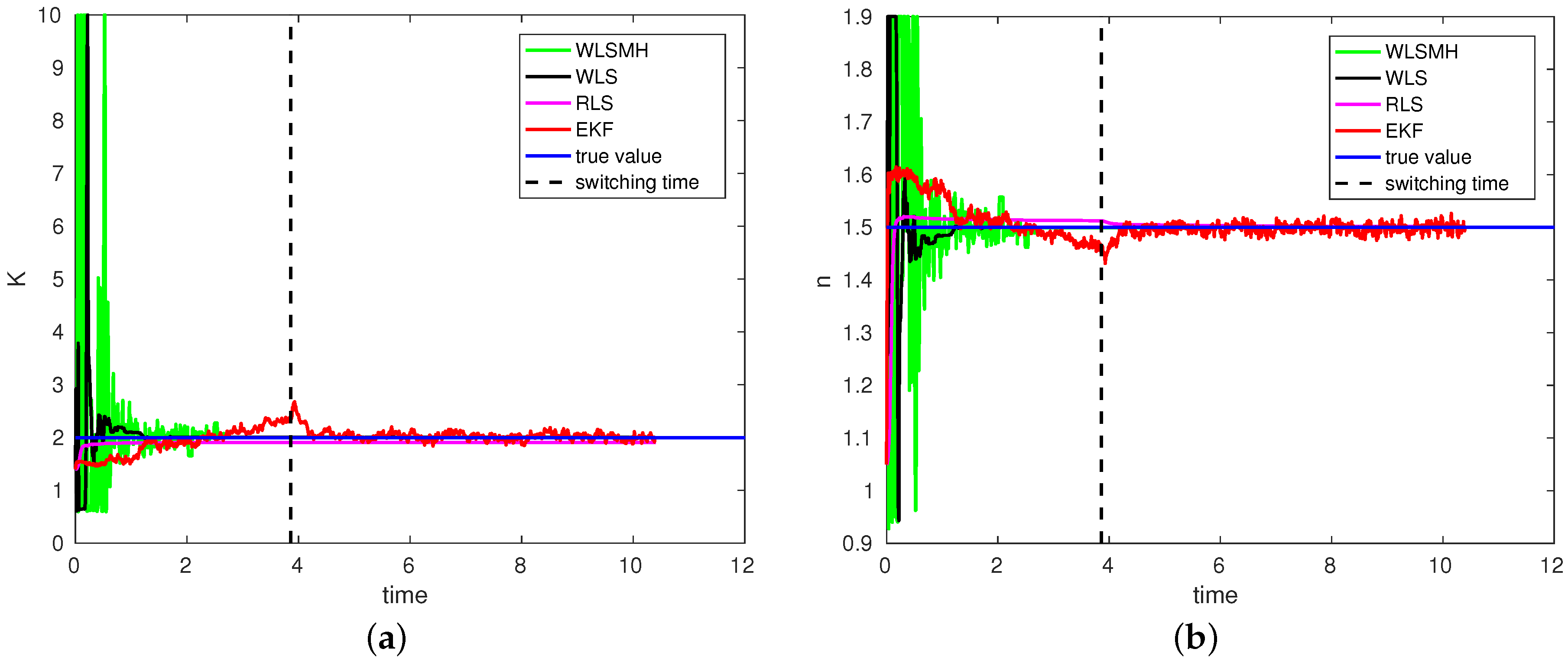
The time-varying profiles of the unknown fouling parameters ($K,n$) are shown in Figure 3. We can observe that in the case of the WLS and WLSMH methods, the parameters converged quickly to a close neighborhood of the true values of the parameters ($K=2$ and $n=1.5$) prior to the switching time (vertical black dashed line) of the optimal control to the singular arc. The WLS method was able to estimate the true values of the parameters in the first few samples. However, in the case of WLSMH, the estimation needed more time, and we can observe that the parameter values were oscillating for the first two hours. This was due to the NLP solver falling into local minima. This can also be attributed to the chosen length of the moving horizon and the possibly imperfect choice of the initial covariance matrix ${\mathit{P}}_0$. To overcome the issue of NLP solver falling into local minima, one can employ global optimizers. However, based on our observations, the local minima were only hit in the first samples of the estimation when only a few measured outputs were considered. When the recursive methods (RLS, EKF) were used, we can observe that the parameters converged almost to the true values of the parameters. The difference in the estimated and true values of the parameters is attributed to the strong nonlinearity of the process model. Moreover, the performance of these methods also strongly depends on the choice of the covariance matrices. Overall, we can conclude that all of the estimation methods were able to estimate the unknown fouling parameters or converge almost to true values of the parameters even before switching to the singular surface where singular control is applied. As a result, the theoretical optimality of the diafiltration process was almost restored when using the proposed estimators and coupling them within the feedback control law. Similar behavior for parameter estimation was also observed for other fouling models.

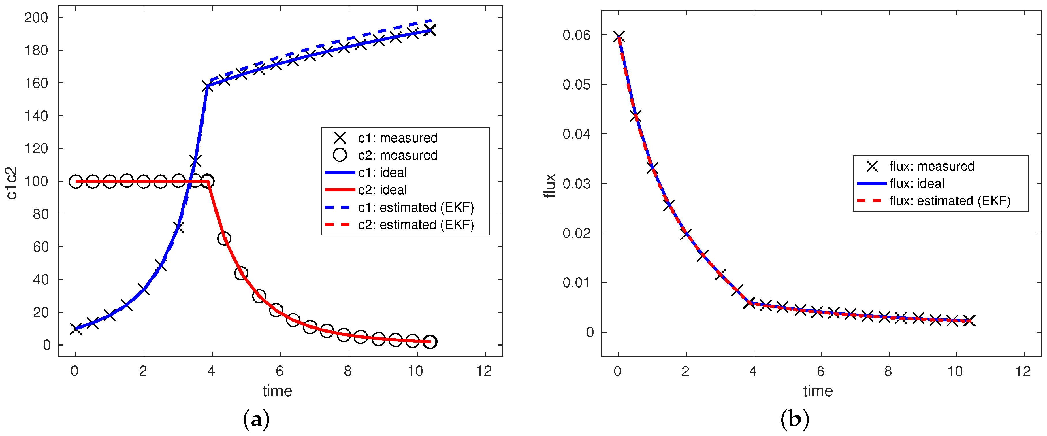
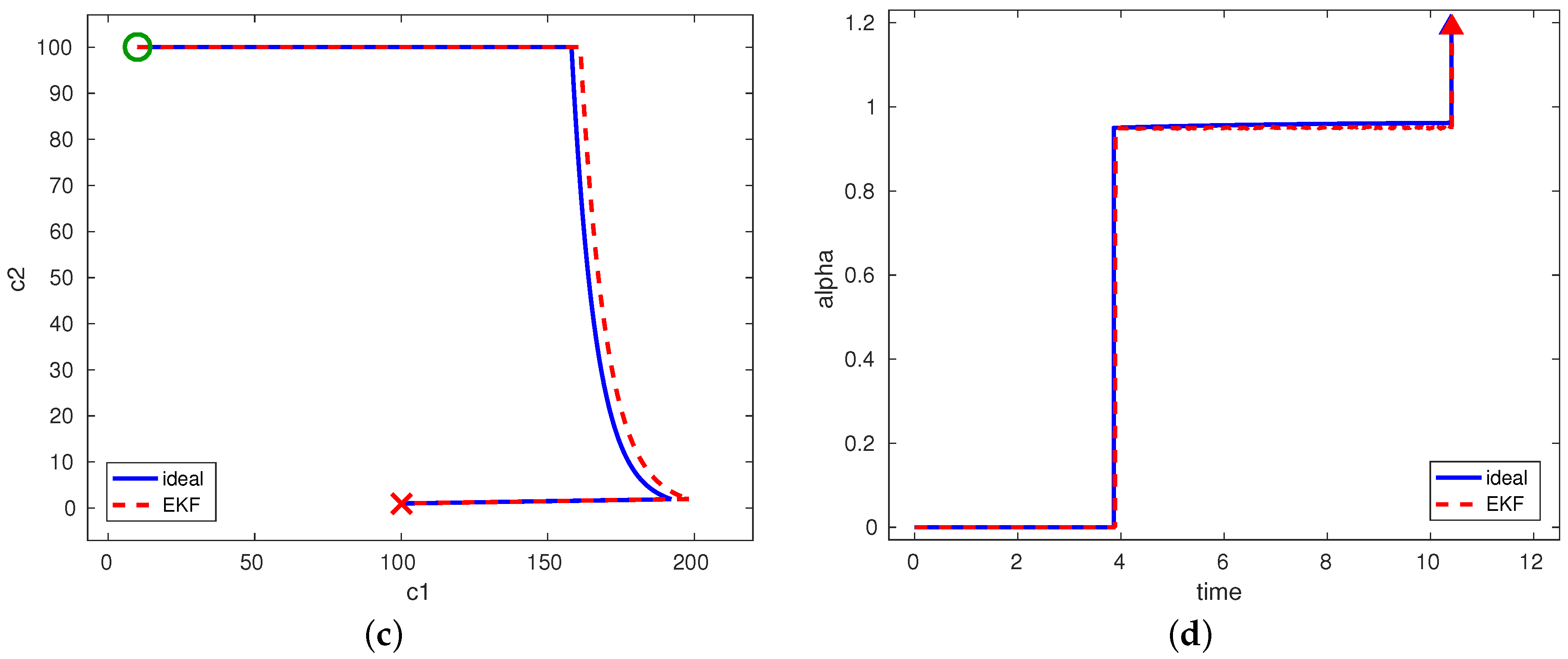
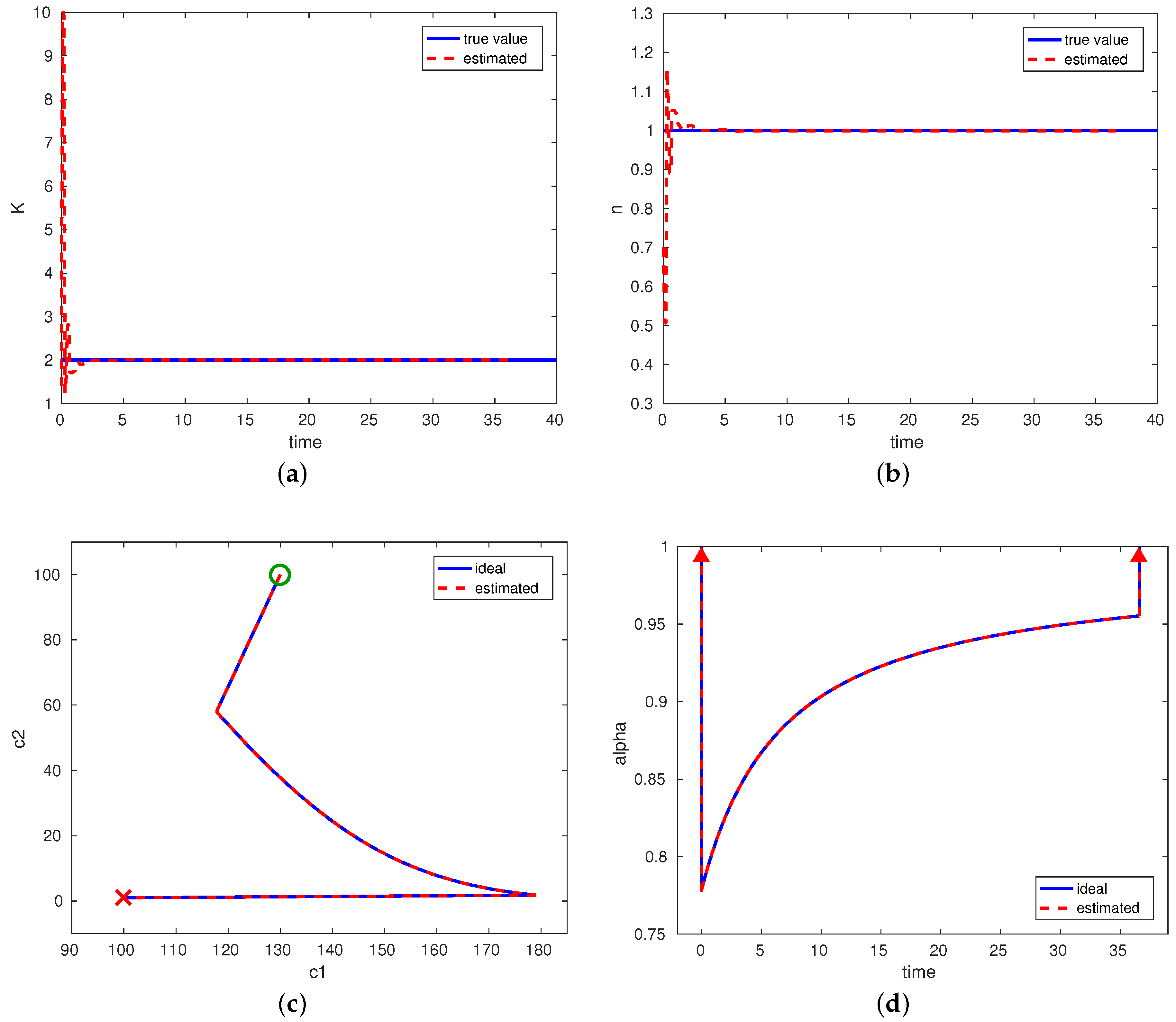
Figure 4 shows the concentration, flux and control trajectories for the ideal and estimated cases together with the considered measurements of concentrations and flux. The figures show only one of the estimation method (EKF) for $n=1.5$ as the worst case scenario since in all other cases, the trajectories are closer to the ideal ones. In Figure 4a, we show the considered measured outputs (denoted by the circle and cross) and the ideal and estimated concentration trajectories. However, due to the small sampling time, we only display some of the measured points. The considered measured flux with ideal and estimated parameters is shown in Figure 4b. Moreover, in Figure 4c,d, the optimal concentration state diagram and the optimal control profile are shown. In all figures, the solid lines represent the optimal scenario with a perfect knowledge of parameters. Further, we can observe that the estimated and ideal trajectories in the first step when the control is constant ($\alpha =0$) are identical. This behavior was expected since the control in the first step does not depend on the unknown fouling parameters. The difference in the second interval is negligible. This was due to the convergence of the parameters during the first step. For this reason, the singular control in the second step is calculated with almost the true value of the parameters. The measured concentration of the macro-solute (blue dashed line in Figure 4a) shows the increasing difference to the ideal one at the singular step. However, this has only a minor impact on the overall optimal operation. Based on the results, we can conclude that by using the estimated parameters obtained by all estimation techniques, the overall operation is very close to optimal one with only minor differences in the processing and switching times. Moreover, it should be also mentioned that even if satisfactory convergence was obtained with the EKF method, different Kalman filter methods, like the unscented Kalman filter [40], could be also employed for the parameter estimation.

Next, we study the case where the initial concentrations are $[c_{1,0},c_{2,0}]=[130\mathrm{mol}/{\mathrm{m}}^3,100\mathrm{mol}/{\mathrm{m}}^3]$, while the same final concentrations have to be met as in the previous cases. The optimal control strategy starts with pure dilution in the first step and in the last step, which follows after an operation on a singular arc. We use the same estimators as before, with the same tuning matrices.

In Figure 5, we show the results of the estimation of the unknown fouling parameters using the WLS method and the corresponding concentration state diagram and control profile of the on-line control strategy. As stated above (Section 4), the entry to the singular arc (50) can be determined without the knowledge of fouling parameters as $J=J_0$. On the singular arc, the estimation of the unknown fouling parameters commences. We can observe in Figure 5a,b that the unknown fouling parameters were estimated accurately in the first three hours of operation where the overall time-optimal operation was approximately 37 hours. The suboptimality of the on-line control strategy w.r.t. the ideal one is ${\delta }_{\mathrm{tf}}^{*}=0.025$. The oscillations in the first minutes of the operation were mainly caused by a small set of measured outputs. A similar behavior was observed in the previous case. Once the amount of measured outputs is increased, we can observe a quick convergence of the estimated parameters towards the true values. The comparison of ideal and estimated concentrations and control trajectories is shown in Figure 5c,d. As we can observe, the differences in the concentrations and control trajectories for ideal and estimated cases are negligible. This is due to the quick convergence of the estimated fouling parameters. We also performed simulations with the rest of the estimation methods.

In the case of the recursive methods (EKF and RLS), by using the same covariance matrices (51) to (54) as in the previous case, the estimated parameters diverged in the first hour of the batch and were not able to converge to the true values of the parameters. The same behavior was also observed in the case of the WLSMH method, since the covariance matrix $\mathit{P}$ was updated based on the EKF method. The reasons for the divergence of the WLSMH, RLS and EKF methods was mainly caused due to the high sensitivity of the choice of the covariance matrices and the strong non-linearities of the process model. Other reasons for the possible divergence issues as discussed in Section 4.3 are the insufficient amount of measured outputs, since the estimation starts at the singular surface, and insignificant sensitivity between the measured outputs and the estimated parameters on the singular surface. This was caused by almost constant flux on the singular surface.

Overall, we can conclude that even if in the first step, pure dilution mode has to be applied and the estimation of unknown fouling parameters is only performed during the singular control, the differences between the ideal and estimated trajectories are negligible. The results indicate that the estimated parameters converged reasonably close to the true values of the parameters in the first hours of operation. For this reason, the overall operation is very close to the optimal one with only negligible differences in the case when the WLS method is applied. However, in the rest of the estimation methods, strong divergence of the estimated parameters was observed.

7. Conclusions

In this paper, we studied the time-optimal operation of a diafiltration process in the presence of membrane fouling. The optimal operation and control is an explicit non-linear control law defined over concentration regions. According to the theory, the optimal operation is defined as a three-step strategy with concentration or pure dilution mode in the first and the last step and with a singular arc in the middle step.

In the paper, we provided a detailed analysis on the problems related to the observation of the parameters based on the measured outputs. Based on the analysis, we conclude that by taking into account the concentrations and flux as measured outputs, both parameters could not be estimated at the same time. Therefore, the derivative of flux w.r.t. to time had to be considered as a new measured outputs. Based on the analysis, four standard parameter estimation methods were discussed for the estimation of the unknown fouling parameters on-line during the separation. The crucial reason for estimating the parameters on-line is that the singular surface and control depend on the fouling parameters. The first two methods (WLS and WLSMH) were able to estimate the parameters exactly, whereas the recursive methods (RLS and EKF) converged almost to the true values of the parameters. However, the convergence was satisfactory and resulted in minor differences in the concentration and control profiles compared to the ideal case. Based on the results, we conclude that by using the EKF estimation method, we improve the convergence with the lowest computational time compared to other discussed methods. If the optimal operation starts with a pure dilution mode, only WLS and WLSMH were able to converge to the true values of the parameters, whereas the recursive methods (RLS and EKF) diverged completely from the true values. A possible remedy for the future could be to inject some dither signal into singular dilution rate to increase the excitation of the process.

All of the results presented in this paper are based on simulation results where the process noise was also considered in the simulations. Future research directions will be focused on experimental implementation of the proposed estimation techniques on a laboratory membrane process.