Artificial Intelligence-Based Oil Well Condition Diagnosis and Production Parameter Optimization

Abstract

To address the challenges of low production efficiency, high energy consumption, and frequent equipment failures in low-producing wells, this study proposes an intelligent production parameter optimization method based on deep learning and multi-indicator fusion. First, a Long short-term memory (LSTM)-based prediction model was developed using the displacement–load characteristics of pumping-unit dynamometer cards. The results show that the model achieves an average prediction metric Q = 0.08, outperforming Back Propagation and Recurrent Neutral Network (BP and RNN) models. Second, a Convolutional Neutral Network (CNN) was employed to extract the fluid supply capability features, achieving a recognition accuracy exceeding 98%, thereby validating the model’s effectiveness. Combined with three types of time series data (liquid supply degree, dynamic liquid level, and liquid production rate), a multi-index fusion parameter optimization method is proposed. A comprehensive decision-making model is constructed based on the Analytic Hierarchy Process (AHP), which takes long-term, short-term, and overall feature changes as the basis, and forms a hierarchical framework by decomposing objectives and quantifying feature weights. The consistency ratio (CR) of the model is less than 0.1, meeting the requirement of logical consistency and enabling the output of standardized regulation suggestions. Consequently, a closed-loop system of “data preprocessing—condition prediction—state identification—parameter optimization” was constructed, enabling early dynamometer card prediction, accurate fluid supply fluctuation identification, and automatic generation of optimization schemes. This system effectively enhances production efficiency and equipment stability in low-producing wells, providing a technical foundation for intelligent oilfield development.

1. Introduction

A low-production oil well refers to an oil well with a daily output below the specific industry standard. In China’s oil and gas development field, there is a huge stock of low-production oil wells, and their efficient development is of great practical significance for ensuring stable oil and gas production, improving efficiency, and enhancing the comprehensive utilization rate of resources. According to statistical data from PetroChina, the average daily output of low-production oil wells in China is approximately 2–3 tons, which generally face the problems of low production efficiency and high unit development cost. Given the wide distribution of oil and gas resources and the complex geological conditions [1], pumping units are widely used in oil and gas extraction because of their strong adaptability, ease of operation, and low cost. As a core monitoring method for the operating state of the pumping system, the dynamometer card intuitively reflects the relationship between load and displacement over a single stroke; by analyzing its morphological features and variation trends, the operating status of sucker rods, pumps, and tubing can be identified, providing a basis for condition assessment [2]. Under complex operating conditions, sucker-rod pump systems are prone to faults such as sand or wax sticking, gas locking, pump leakage, and rod breakage or separation, which not only reduce production but also increase equipment risk [3]. Predictive analysis based on dynamometer cards can extract features and identify faults to support fault localization and production parameter optimization, enabling early warning and dynamic control, thereby significantly improving system safety, stability, and efficiency [4]. In recent years, dynamometer card recognition methods have developed rapidly. Traditional methods rely on manual feature extraction and rule matching—such as shape analysis, template matching, and statistical pattern recognition—which are limited by expert experience and have poor generalization; theory-based methods simulate faults by building the working principles and mathematical models of the sucker-rod system [5]; overall, traditional approaches that depend on manual analysis or template matching have low accuracy and poor flexibility in complex scenarios [6].

With the development of machine learning and deep learning, methods such as Support Vector Machine (SVM) and random forest have been applied to dynamometer card classification to improve recognition accuracy [7]. Recently, Convolutional Neural Network (CNN) has shown outstanding performance in extracting spatial features from image-like dynamometer cards, while Recurrent Neutral Network (RNN) and its variant Long short-term memory (LSTM) are adept at processing time series data; attention mechanisms and transfer learning offer new solutions for small-sample and cross-field recognition scenarios [8,9,10]. Zhang, K. et al. [11] used deep autoencoders for an intelligent diagnosis of rotating machinery. Liu J. et al. [12] proposed optimizing the Chicken Swarm Optimization (CSO) algorithm with differential mutation and an adaptive inertia strategy (DACSO) to optimize an SVM model, achieving low production fault diagnosis via dynamometer card classification; Yu, D. et al. [13] extracted key features from progressive cavity pump operation data to build an SVM-based operating-state recognition model and validated it with experimental simulation platform measurements, showing good diagnostic performance. Liu, S. et al. [14] proposed a method for early fault detection in sucker-rod systems by monitoring operating parameters and applying the AdaBNet algorithm to improve accuracy, which can enhance asset monitoring, extend well life, reduce maintenance costs, and enable remote monitoring and prediction of potential issues, though the model has poor interpretability and requires large amounts of training data. In recent years, deep-learning-based fault diagnosis methods, particularly convolutional neural networks, have been used for pumping unit state recognition. Compared with methods such as random forest (RF), k-nearest neighbors (k-NN), spectral clustering, and density peak clustering (DPC), deep learning techniques demonstrate much stronger pattern-mining capability in scenarios with many features, low signal sensitivity, and complex data types, and have been widely applied in object detection, image recognition, behavior prediction, 3D reconstruction, and visual relocalization [15,16,17,18,19,20].

Furthermore, deep learning methods can automatically extract image features from dynamometer cards using deep neural networks [21]; Moghimihanjani, M. et al. [22] and Dong, L. et al. [23] applied CNNs for bearing fault diagnosis, showing that CNNs have become leading architectures and perform well across many tests. Peng, Y. et al. [24] proposed a CNN-based method for dynamometer card recognition, classifying cards under different conditions with good results. He, Y.-P. et al. [25] proposed a capsule-network-based method for pump dynamometer card recognition; capsule networks are a novel deep learning model able to better capture feature relationships in graphics. Shan, L. et al. [26] used an improved CNN-BiLSTM model for well production forecasting; this model combines convolutional neural networks and bidirectional LSTM to effectively predict well performance. [27] proposed both image-based and data-based CNN methods, confirming that CNN-based approaches yield higher recognition accuracy than machine learning algorithms like random forest and k-NN. Daolun, L.I. et al. [28] also validated the effectiveness of image-based CNNs in well fault classification. Although BP neural networks are suitable for static data tasks, they lack temporal memory and the ability to capture time-dependent relationships due to structural limitations, failing to adapt to the dynamic characteristics of dynamometer cards and resulting in insufficient prediction accuracy. Traditional RNNs, while specifically designed for temporal data, struggle to maintain long-term memory due to gradient vanishing and gradient exploding issues, being only applicable to short-time sequences and exhibiting limited performance when dealing with complex long-time sequences. In contrast, LSTM networks, endowed with excellent long-term dependency processing capabilities by their gating mechanisms, can accurately capture key temporal features and adapt to complex dynamic patterns of data. They demonstrate significant advantages in dynamometer card prediction for oil wells, providing an ideal model choice for the accurate prediction of full-cycle dynamometer cards.

The degree of liquid supply in a well reflects the ratio of actual fluid output to the theoretical maximum output and can be preliminarily judged by indicators such as production and water cut; it is important for improving production efficiency [29,30,31], reducing energy consumption, and optimizing field development. Traditional measurement methods are complex, have poor real-time performance, and are easily disturbed. Andrade, G.M.P. et al. [32] analyzed the principles and pros and cons of various flowmeters and downhole test tools and proposed improvements, laying a foundation for modern measurement technologies and AI development; Zhong, Z. et al. [33] designed a monitoring system based on surface sensors that judges the liquid supply degree of low-producing wells from wellhead pressure, temperature, and other parameters—this system is simple to install and maintain and has been field-validated. Han, D. et al. [34] built a liquid supply recognition model based on machine learning that predicts low-producing well supply conditions from historical production and real-time monitoring data, showing high predictive accuracy and generalization. The above methods generally suffer from model complexity and the need for large sets of operating parameters, highlighting the potential of deep learning for predicting liquid supply in low-producing wells.

Research on production parameter optimization for low-producing wells is mainly divided into mechanism-based modeling and data-driven approaches. Weiwei, T. et al. [35] proposed a mechanism-simulation-based parameter optimization method for sucker-rod pump lifting systems, using big data analysis to increase production and reduce energy consumption, and combined simulation with field data to build deep learning models that recommend efficient schemes; however, adaptability across different geological conditions is limited. Wang, H. et al. [36] used multiple machine-learning algorithms to build models relating production parameters and output and improved well production through parameter optimization. Dong, Y. et al. [37] proposed a curve-adaptive and simulated annealing particle swarm optimization algorithm that takes production time, injection volume, and bottom hole flow pressure as inputs and optimizes injection production parameters to maximize net present value. Data-driven methods integrate multi-source data and continuously update models to achieve ongoing production parameter optimization and significantly improve well production efficiency.

In summary, this paper constructs an AI-based research approach to address the full process needs of low-producing wells-“condition diagnosis liquid supply recognition parameter optimization.” In this study, LSTM neural networks are used to model the time series features of dynamometer cards to improve prediction accuracy; a high-precision liquid supply recognition model is established by combining CNNs with an iterative labeling method; and the Analytic Hierarchy Process (AHP) is introduced to integrate multi-indicator time series features, constructing a long- and short-term fused comprehensive decision model to achieve quantitative optimization of production parameters. This method aims to overcome current technical shortcomings in adaptation to complex operating conditions and multi-indicator coordinated control, and it has important research value and application potential for intelligent operation and maintenance of low-producing wells.

2. Materials and Methods

2.1. Backpropagation Neural Network (BP)

Training of a BP neural network alternates between forward propagation and backpropagation: forward propagation computes outputs layer by layer from the inputs, while backpropagation updates weights based on the error between predictions and target values to achieve learning [38]. For the same training set, model performance can be tuned by selecting different activation functions and parameters. The BP principle is shown in Figure 1.

The error function is:

$$e={\displaystyle \frac{1}{2}}{\displaystyle \sum _{k=1}^a{\left[d_o(k)-y_o(k)\right]}^2}$$

(1)

Randomly select the K-th input sample and the corresponding desired output:

$$x(k)=(x_1(k),x_2(k)\cdots x_n(k))$$

(2)

$$d\left(k\right)=\left(d_1\left(k\right),d_2\left(k\right)\cdots d_n\left(k\right)\right)$$

(3)

For each neuron in a hidden layer, compute its input and output:

$$h{i}_{\mathrm{h}}\left(k\right)={\displaystyle \sum _{i=1}^n{w}_{\mathrm{ir}}}{x}_{\mathrm{i}}\left(k\right)-b_{\mathrm{a}},h=1,2,\cdots p$$

(4)

$$h{o}_{\mathrm{h}}\left(k\right)=f\left(h{i}_{\mathrm{n}}\left(k\right)\right),h=1,2,\cdots p$$

(5)

$$y{i}_o\left(k\right)={\displaystyle \sum _{i=1}^p{w}_{bo}}h{o}_n\left(k\right)-b_o,o=1,2,\cdots q$$

(6)

$$y{o}_o=f\left(y{i}_o\left(k\right)\right),o=1,2,\cdots q$$

(7)

Using the network’s expected outputs and actual outputs, compute the partial derivatives of the error function with respect to the output layer neurons, applying the chain rule:

$${\displaystyle \frac{\partial e}{\partial h{i}_h\left(k\right)}}=-{\delta }_h\left(k\right)$$

(8)

$${\displaystyle \frac{\partial e}{\partial w_{ho}}}=-{\delta }_h\left(k\right)h{o}_h\left(k\right)$$

(9)

The output layer neuron ${\delta }_h\left(k\right)$ and the hidden layer neuron output $w_{ho}(k)$ are used to modify the connection weights, then:

$$\Delta w_{ho}(k)=-\mu {\displaystyle \frac{\partial e}{\partial w_{ho}}}=\mu {\delta }_h(k)$$

(10)

$$w_{ho}^{N+1}=w_{ho}^N+\eta {\delta }_o\left(k\right)h{o}_h\left(k\right)$$

(11)

In the formula, $\mu$ and $\eta$ represent learning rates; by adjusting the step size, one can avoid divergence caused by overly large updates and approach the optimal solution.

Use the deltas of the hidden layer neurons ${\delta }_h\left(k\right)$ and the inputs of the input layer neurons to correct the connection weights:

$$\Delta w_{ih}\left(k\right)=-\mu {\displaystyle \frac{\partial e}{\partial w_{ih}}}={\delta }_h\left(k\right)x_i\left(k\right)$$

(12)

$$w_{ih}^{N+1}=w_{ih}^N+\eta {\delta }_h\left(k\right)x_i\left(k\right)$$

(13)

Compute the global error:

$$E={\displaystyle \frac{1}{2m}}{\displaystyle \sum _{i=1}^m{\displaystyle \sum _{o=1}^a{\left[d_o(i)-y_o(i)\right]}^2}}$$

(14)

Evaluate the network error; the algorithm terminates when this error reaches a preset accuracy or exceeds a preset maximum number of iterations N.

2.2. Recurrent Neural Network (RNN)

A recurrent neural network (RNN), proposed by Elman [39], is a neural network for processing sequential data and is suitable for sequences such as natural language, audio, and stock trends. Its core is that the hidden layer input fuses the current input with the previous time step’s hidden layer output, enabling the capture of temporal information and learning of sequence nonlinearities. The RNN principle is shown in Figure 2.

Figure 3: Schematic diagram of a Recurrent Neural Network (RNN) recurrent cell. As shown in the figure, the core unit of an RNN is the recurrent cell, whose structure is similar to a fully connected layer. Although the weight matrices for the current input ($x_t$) and the previous hidden output ($h_{t-1}$) are shown separately as $W_x$ and $W_h$, this is equivalent to concatenating $x_t$ and $h_{t-1}$ and then applying a single parameter matrix. Key components are defined as follows: (a) $h_{t-1}$: Previous hidden state, representing the memory information passed from the last time step; (b) $x_t$: Input data at the current time step; (c) tanh: Activation function that introduces non-linearity to transform the combined input and hidden state; (d) $h_t$: Hidden state at the current moment, the output of the RNN unit carrying both current input and historical information, which is also passed to the next time step. Abbreviations: RNN = Recurrent Neural Network. The mathematical expression is:

$$h_t=\sigma (W_x{x}_t+W_h{h}_{t-1}+b)$$

(15)

which can also be written as:

$$h_t=\sigma (W[x_t°h_{t-1}]+b)$$

(16)

In the formula, $°$ denotes vector concatenation.

The components are labeled as follows: (a) $h_{t-1}$: Hidden state at the previous time step, representing the memory information passed from the last moment. (b) $x_t$: Input data at the current time step. (c) $W_h$: Weight matrix for the hidden state input. (d) $W_x$: Weight matrix for the current input data. (e) σ: Sigmoid activation function, which introduces non-linearity to transform the combined input and hidden state. (f) $O_t$: Output at the current time step, generated by the activation function processing. (g) $h_t$: Hidden state at the current time step, carrying both current input and historical information, and passed to the next time step.

2.3. Long Short-Term Memory (LSTM)

The Long Short-Term Memory (LSTM) neural network is a special form of Recurrent Neural Network (RNN). Built on the foundation of multi-layer feedforward networks, RNN achieves memory functionality by transmitting information from the previous time step through lateral connections of hidden layers and weight matrices [40]. Through the synergistic design of three core gating units (Forget Gate, Input Gate, Output Gate) and a Cell State, LSTM effectively addresses the vanishing gradient problem of traditional RNNs. It can accurately capture and retain key information as well as temporal dependencies in long time series, dynamically adapt to complex fluctuations of data while preserving long-term critical features, and break through the inherent limitation of RNNs that only support short-term memory, ultimately delivering more accurate and stable prediction results; The LSTM workflow is shown in Figure 4.

By designing three core gating units (Forget Gate, Input Gate, Output Gate) and a Cell State, the network effectively alleviates the vanishing gradient problem faced by traditional Recurrent Neural Networks (RNNs) in long-sequence modeling, enabling accurate storage and transmission of long-term dependent information: (a) Forget Gate, composed of a Sigmoid activation function layer, whose output vector acts on the previous cell state ($C_{\iota -1}$) through element-wise multiplication to adaptively filter out redundant historical information; (b) Input Gate, synergistically constituted by a Sigmoid layer and a tanh layer: the Sigmoid layer outputs an update weight vector for selecting key information to be integrated into the cell state; the tanh layer generates a candidate cell state ($C_t$) with a value range of [−1, 1], and the two complete the cell state update through element-wise multiplication and addition operations; (c) Output Gate, composed of a Sigmoid layer and a tanh layer: the Sigmoid layer outputs a filtering vector to filter information from the current cell state ($C_t$); the tanh layer normalizes the filtered cell state to the [−1, 1] interval, ultimately generating the current hidden state ($h_t$) while transmitting the updated cell state ($C_t$) to the LSTM unit at the next time step.

Abbreviations: LSTM = Long Short-Term Memory; RNN = Recurrent Neural Network; $C_{\iota -1}$ = Previous Cell State; $C_t$ = Current Cell State; $x_t$ = Current Input Feature Vector; $C_t$ = Candidate Cell State; $h_t$ = Current Hidden State.

Forget gate (selectively forgets information in the cell state):

$$f_{\iota }=\sigma [W_f(h_{\iota -1},x_{\iota })+b_f]$$

(17)

Input gate (selectively records new information into the cell state):

$$i_{\iota }=\sigma [W_i(h_{\iota -1},x_{\iota })+b_i]$$

(18)

$${\tilde{C}}_{\iota }=\tanh [W_c(h_{\iota -1},x_{\iota })+b_c]$$

(19)

Cell state update:

$$C_{\iota }=f_{\iota }{C}_{\iota -1}+i_{\iota }{\tilde{C}}_{\iota }$$

(20)

Output gate (controls the output based on input and cell state, and updates the next hidden state):

$$o_t=\sigma \left[W_o\left(h_{t-1},x_t\right)+b_o\right]$$

(21)

$$h_{\iota }=o_{\iota }\tanh C_{\iota }$$

(22)

In the formula, $x_{\iota }$ is the input information of the current moment; $W_f$, $W_i$, $W_C$, $W_o$ are the weights of forgetting gate, input gate, memory unit and output gate, respectively; $b_f$, $b_i$, $b_C$, $b_o$ for the corresponding bias.

2.4. Convolutional Neural Network (CNN)

A convolutional neural network (CNN) is a deep learning architecture specifically designed for data with a known grid structure. It can excavate complex structures in the data, which gives it high robustness to small perturbations in the input [41]. The CNN principle is shown in Figure 5.

The convolutional neural network (CNN) consists of an input layer (image), convolution + ReLU layers, a max-pooling layer, a fully connected layer, and an output layer. The image recognition process, the data flow between the layers (indicated by arrows in the diagram), and the meaning of the colors are as follows:

The input layer receives the raw image data (represented in purple in the diagram, corresponding to the original image block), which is then passed through an arrow to the convolution + ReLU layer. The feature maps generated by this layer are shown in cyan, with the light green patches within the cyan areas representing the local feature regions extracted via convolution. In this layer, convolution operations extract local features, and the ReLU activation function introduces nonlinearity to enhance the feature representation capability, ultimately generating multiple feature maps.

These cyan feature maps are then passed through an arrow to the max-pooling layer, where the output feature maps are displayed in orange. The pink patches within the orange areas correspond to the key features retained after down-sampling. This layer reduces dimensionality via down-sampling while preserving important features and enhancing the network’s translation invariance, resulting in smaller feature maps.

The pooled orange feature maps are then "flattened" and passed (via an arrow) to the fully connected layer, where the nodes are shown in dark green (with gradient effects to represent the process of feature integration). In this layer, the features are integrated, establishing a mapping between the features and output classes for classification computation.

Finally, the classification result computed by the fully connected layer is passed through an arrow to the output layer (represented in light blue, with yellow circular nodes indicating the output classification nodes). The output layer then outputs the classification result, completing the image recognition task.

(1)

Convolutional layer

The convolutional layer is the core of a CNN and is used for feature extraction. It applies learnable filters that slide over the input and perform dot product operations on local regions to produce two-dimensional activation maps (feature maps) [42].

The convolution operation is:

$$O(i,j)=(I^{*}K)(i,j)={\displaystyle \sum _{m=0}^{M-1}{\displaystyle \sum _{n=0}^{N-1}I}}(i+m,j+n)·K(m,n)$$

(23)

In the formula, $I(i,j)$ is the value of the input image at position $(i,j)$; $K(m,n)$ is the filter value at position $(m,n)$; $m$ and $n$ are the filter height and width; and $O(i,j)$ is the output value at position $(i,j)$.

(2)

Pooling layer

The pooling layer reduces the spatial dimensions of feature maps, lowers computational cost, and increases robustness to feature position shifts:

$$y(i,j)={\max }_{m,n}x(i·s+m,j·s+n)$$

(24)

In the formula, $x$ is the input feature map; $y$ is the pooled output feature map; $s$ is the stride; $(m,n)$ indexes positions inside the pooling window.

(3)

Fully connected layer

After several convolutional and pooling layers, one or more fully connected layers are used for classification or other tasks. In these layers, the network integrates all previously extracted features to produce the final outputs.

(4)

Output layer

The output from the last fully connected layer is fed to the output layer, typically a softmax layer, which yields class probabilities; the class with the highest probability is taken as the prediction.

2.5. Analytic Hierarchy Process (AHP)

The Analytic Hierarchy Process (AHP) [43], developed by Thomas L. Saaty, is an important multi-criteria decision-making method. It decomposes a complex problem into hierarchical levels and factors, builds a judgment matrix by pairwise comparisons, computes the eigenvector to determine alternative weights, and thereby provides a basis for optimal decision-making. AHP is widely used in management, project evaluation, resource allocation, and risk assessment. The hierarchy model is shown in Figure 6.

The analytic hierarchy process (AHP) model is constructed as a three-level architecture from top to bottom, including the Decision-Making Objectives layer, Pre-test Items layer (Pre-test 1~i), and Decision Alternatives layer (Decision 1~j): By decomposing complex decision-making objectives into several pre-test items level by level, systematic analysis is conducted based on the correlation between pre-test items and decision alternatives. Through pairwise comparisons, a judgment matrix is constructed, and eigenvectors are calculated to determine the weight of each alternative, ultimately achieving hierarchical and quantitative decision-making for complex problems.

(1)

Constructing the judgment matrix

For n elements at a given level $C_1,C_2,\dots ,C_n$, pairwise comparisons produce an n × n matrix A, i.e., the judgment matrix:

$$A={\left(a_{ij}\right)}_{n\times n}=\left(\begin{array}{cccc}{a}_{11}& a_{12}& \cdots & a_{1n}\\ a_{21}& a_{22}& \cdots & a_{2n}\\ ⋮& ⋮& \ddots & ⋮\\ a_{n1}& a_{n2}& \cdots & a_{nn}\end{array}\right)$$

(25)

In the formula, $a_{ij}$ denotes the importance scale of element $C_i$ relative to $C_j$. This matrix must satisfy two conditions to form a positive reciprocal matrix.

(2)

Calculating the weight vector

Geometric mean method (root method):

$$W_i={\displaystyle \frac{{({\displaystyle \prod _{j=1}^n{a}_{ij}})}^{1/n}}{{\displaystyle \sum _{i=1}^n{({\displaystyle \prod _{j=1}^n{a}_{ij}})}^{1/n}}}},i=1,2,\dots ,n$$

(26)

Arithmetic mean method (sum method):

$$W_i={\displaystyle \frac{1}{n}}{\displaystyle \sum _{j=1}^n\frac{a_{ij}}{{\displaystyle \sum _{k=1}^n{a}_{kj}}}},i=1,2,\dots ,n$$

(27)

3. Results and Discussion

3.1. Data Preprocessing and Selection of Dynamometer Card Prediction Method

3.1.1. Data Preprocessing

This study uses 500 measured dynamometer cards continuously collected from a production plant in Oilfield X as the original time series data. The acquisition parameters were set to 200 sampling points per dynamometer and a sampling interval of 20 min. With extended pumping time, the “handle” shape of low-producing wells’ dynamometer cards gradually elongates, showing a temporal trend that is valuable for prediction studies.

A dynamometer card consists of the polished rod (suspension point) displacement and the load; both are sampled at fixed time intervals within a single stroke, but displacement data vary between cards. Predicting displacement directly would increase model complexity, so interpolation is used to fix displacement sampling points and predict only the load.

The specific processing steps are as follows: first, take the maximum displacement as the midpoint and divide a single stroke into upstroke and downstroke; then set the number of interpolation points to 100 and compute the interpolated displacement points sequentially according to Equation (28); finally, apply cubic spline interpolation to complete the data processing.

$$x[0,100]=range(0,x_m,{\displaystyle \frac{x_m}{99}})$$

(28)

In the formula, $x[0,100]$ denotes the interpolated sequence and $x_m$ is the maximum displacement.

$$S_i(x)=a_i+b_i(x-x_i)+c_i{(x-x_i)}^2+d_i{(x-x_i)}^3$$

(29)

In the formula, $i$ is the segment spline, each segment spline is defined in [$x_i$, $x_{i+1}$], and its coefficient $a_i$, $b_i$, $c_i$, $d_i$ is determined by the following constraints:

(1)

Interpolation condition: the spline must pass through the end-point data;

(2)

Continuity condition: function values and first derivatives are continuous at joints;

(3)

Smoothness condition: second derivatives are continuous at joints;

(4)

Boundary conditions: endpoints X₀ and X_n must have specified boundary conditions. This yields dynamometer card data with fixed displacement and variable load, which are then normalized.

Because different physical quantities have widely different scales, direct modeling can cause biased regression coefficients, reduced prediction accuracy, and poor generalization. To improve prediction accuracy, data must be standardized before the correlation analysis. Max–Min normalization was applied to rescale the load values to the [0,1] interval, thereby improving the efficiency and stability of subsequent network training [9]. The mathematical expression is given in Equation (30). The preprocessed upstroke and downstroke dynamometer cards are shown in Figure 7 and Figure 8, respectively.

$$X_1={\displaystyle \frac{X-X_{\min }}{X_{\max }-X_{\min }}}$$

(30)

In the formula, X₁ is the normalized data, X is the original data, X_min is the minimum of the original data, and X_max is the maximum of the original data.

Figure 7 and Figure 8, respectively, depict the dynamic variation relationship between payload and displacement during the upstroke and downstroke processes: the upstroke curve shows a rapid upward trend of payload in the initial stage of displacement (within a small range) and then enters a fluctuating stable phase, reflecting the evolutionary characteristic of the mechanical response transitioning from drastic change to stability at this stage; the downstroke curve first exhibits slight fluctuations, and when the displacement approaches 1.0, the payload presents a sharp upward tendency, which reveals the non-linear response law of the payload-displacement during the downstroke phase. Together, these two curves clearly demonstrate the phase-dependent variation characteristics of the payload-displacement relationship throughout the full stroke, providing robust support for the dynamic response analysis of pumping units.

3.1.2. Dynamometer Card Prediction Methods and Evaluation Metrics

(1)

Evaluation metrics

To evaluate the model performance, mean squared error (MSE), mean absolute error (MAE), and the coefficient of determination (R²) are used. MAE reflects model robustness, MSE characterizes the overall error level, and R² measures goodness of fit. In addition, a metric Q is defined as the mean of the squared errors between the predicted load sequence (normalized values) and the true values—a lower Q indicates higher prediction accuracy. The metrics are computed as:

$$\mathrm{MSE}={\displaystyle \frac{1}{n}}{\displaystyle \sum _{i=1}^n{(y_i-{\widehat{y}}_i)}^2}$$

(31)

$$\mathrm{MAE}={\displaystyle \frac{1}{n}}{\displaystyle \sum _{i=1}^n\left|y_i-{\widehat{y}}_i\right|}$$

(32)

$$R^2=1-{\displaystyle \frac{{\displaystyle \sum _i{\left({\widehat{y}}_i-y_i\right)}^2}}{{\displaystyle \sum _i{\left({\overline{y}}_i-y_i\right)}^2}}}$$

(33)

In the formula, $y_i$, ${\widehat{y}}_i$, ${\overline{y}}_i$ are true value, predicted value and average true value, respectively, and n is the number of samples.

$$Q={\displaystyle \frac{1}{I}}{\displaystyle \sum _{i=1}^I{\displaystyle \sum _{j=1}^{200}{\left(y_{ij}-{\widehat{y}}_{ij}\right)}^2}}$$

(34)

In the formula, $I$ is the length of the model output sequence, that is, the number of predicted indicator diagrams; $y_{ij}$ is the first load value of the first real indicator diagram; is the first load value in the corresponding predicted indicator diagram.

(2)

Optimization of prediction methods

According to the same input and output sequence, BP neural network, RNN and LSTM are used to predict the oil well indicator diagram, respectively. The prediction comparison results are shown in

Table 1. Average performance evaluation of each prediction model.

Indicators	LSTM	RNN	BP
Average mean square error	0.1586	0.1954	0.2012
Q	0.018	0.372	1.254

and Figure 9.

From Table 1 and Figure 9, it can be seen that the LSTM model outperforms the RNN and BP neural networks in mean squared error (MSE = 0.1586) and the prediction metric Q (Q = 0.018). The comparison shows that LSTM’s predictions are closer to the measured values, exhibiting the smallest errors and demonstrating its superiority in dynamometer card prediction.

As shown in Figure 10, the loss trend during model training further validates the model’s high accuracy. Moreover, LSTM’s gating mechanisms enable it to effectively capture long-term dependencies in the data, outperforming RNNs that are prone to vanishing gradients and BP networks that lack temporal memory. Considering these factors, the LSTM model was ultimately chosen for dynamometer card prediction.

3.2. LSTM-Based Dynamometer Card Prediction Model

3.2.1. Model Structure Design

The dynamometer card prediction workflow consists mainly of model training and forecasting.

Step 1—training set construction: process the collected dynamometer cards from low-producing wells with sampling interval T = 20 min; use k = 10 dynamometer cards as the time window to predict the next t = 5 dynamometer cards. A sliding window method with stride 1 is employed, producing 486 samples from N = 500 original dynamometer cards.

Step 2—interpolation and normalization: since dynamometer cards evolve over time, normalizing is performed using the maximum displacement and maximum load of the first card in each group, and cubic spline interpolation is applied to unify sampling.

Step 3—LSTM-based sequence-to-sequence prediction: the sequence-to-sequence model built with LSTM is shown in Figure 11. It predicts load data Y and combines them with fixed displacements to form predicted dynamometer cards. The model takes current and historical load sequences Z as input and future load sequences Y as output; the input length is controlled by k = 10 (10 normalized, interpolated load traces, approximately 2000 values) and the output length by I = 5 (5 normalized, interpolated load traces, approximately 1000 values). Considering the comprehensive input–output scale (2000→1000 values) and the temporal characteristics of the load sequence, the optimal number of LSTM layers is one. This structure can effectively extract temporal features and possesses a robust long-term prediction capability.

Both inputs and outputs are load sequences of dynamometer cards: each sample’s input is the preceding k = 10 load sequences and the output label is the following I = 5 load sequences. The loss function is mean squared error (MSE). Hyperparameter settings, which significantly affect robustness and performance, are listed in

Table 2. Prediction model hyperparameters.

Hyperparameter	Setting Value
Learning rate	0.01
Epochs	50
Batch size	8
Optimizer	Adam (betas = (0.9, 0.999), eps = 1 × 10−8, weight dec ay = 0)

.

3.2.2. Sensitivity Analysis of Prediction Model Parameters

Conducting sensitivity analysis on the LSTM-based dynamometer card prediction model helps determine the optimal input and output sequence lengths, thereby improving prediction accuracy and computational efficiency. The analysis can identify information redundancy introduced by overly long input sequences and thereby simplify the model architecture and reduce unnecessary computational overhead; it also helps detect and avoid overfitting caused by excessively long inputs, thus safeguarding the model’s generalization to unseen data. Properly optimizing the input sequence length can substantially reduce inference time and speed up predictions, which is especially beneficial for real-time or near-real-time applications.

In addition, sensitivity analysis can reveal potential prediction instability when the output sequence is too long, ensuring the reasonableness and credibility of model outputs. Based on these considerations, sensitivity analyses were performed along two dimensions—the input sequence length k and the output sequence length I—to determine k and I values suitable for on-site use in low producing wells.

(1)

Sensitivity analysis of input load-sequence length

To improve the accuracy of the dynamometer card prediction model for low-producing wells, an initial input load sequence length was selected empirically and then refined via sensitivity analysis. During the analysis, the output sequence length, model structure, training parameters, and sampling interval were held constant. Considering that the dynamometer card of low-producing wells changes rapidly, the value range of the input load sequence length k is set to 1–10 with a step size of 1; the output load sequence length l is fixed at 5. The resulting variation in the model’s Q metric with k is shown in Figure 12.

As the input load sequence length K increases, the prediction performance metric Q generally decreases, with a pronounced inflection at K = 4. Combined with the variation in Q with k shown in

Table 3. The variation in Q value of indicator diagram prediction model with K value.

K Value	1	2	3	4	5	6	7	8	9	10
Q	11.41	4.12	1.59	0.36	0.13	0.13	0.09	0.09	0.09	0.09

for the dynamometer chart prediction model, the optimal input sequence length under the conditions of this study is K = 5. For smaller K values the model is highly sensitive to changes in K and exhibits large performance fluctuations, which is consistent with the rapid evolution characteristics of dynamometer charts from low-producing wells; once K exceeds a certain threshold, Q tends to stabilize. The Q index essentially reflects the relative deviation between the predicted oil well production and the on-site actual production. It serves as a core engineering indicator for quantifying the prediction accuracy of the model, with smaller values indicating that the predicted results are closer to the actual production and the model is more reliable.

In summary, an input sequence that is too short cannot fully capture the trend information of the dynamometer chart, whereas an excessively long sequence tends to introduce data redundancy and provides limited improvement in prediction accuracy.

(2)

Sensitivity analysis of output load sequence length

In the experiment, the LSTM-based dynamometer chart prediction model keeps the input sequence length fixed at k = 5, while the output sequence length I is varied over I ∈ [1,10] with a step size of 1; the prediction metric Q is recorded for each I (Figure 13).

The results show that Q increases with I and that the growth rate accelerates; pronounced inflection points occur at I = 5 and I = 8, after which the curve’s slope increases markedly. Combining the Q values in

Table 4. Variation in the dynamometer-chart prediction model’s Q value with I.

I Value	10	9	8	7	6	5	4	3	2	1
Q	0.23	0.18	0.15	0.14	0.12	0.10	0.10	0.09	0.09	0.08

and considering overall predictive performance and prediction horizon, I = 5 is chosen as the optimal output sequence length, as this setting ensures a relatively long prediction period while maintaining low prediction error.

3.2.3. Model Prediction Results Validation

Using actual dynamometer charts as examples, the prediction performance is compared and analyzed. Five consecutive historical dynamometer charts ending at time T were selected, normalized, and resampled to a unified sampling interval (30 min) using cubic spline interpolation. The superimposed normalized continuous dynamometer charts are shown in Figure 14.

In the figure, “T” denotes the current dynamometer chart, “1T prior” denotes the previous sampling interval (30 min), and so on up to “4T prior.” As shown in Figure 14, the closed area in the lower left of the dynamometer chart gradually decreases over time, indicating a reduced degree of pump fill-up and a marked weakening of the well’s fluid supply capacity. This trend directly reflects the impact of formation energy depletion on the pumping system’s fluid delivery condition.

Based on the preceding sensitivity analysis, both the input and output sequence lengths of the LSTM model were set to k = 5 and l = 5. The sequence of consecutive historical dynamometer charts was fed into the model to predict dynamometer chart evolution over the next 5T. Figure 15 and Figure 16 presents the comparison between predicted and measured dynamometer charts. Although the predicted curves show minor fluctuations at some time points relative to the measured curves, the overall shape features remain highly consistent, and key evolving features such as the “knife-handle” are effectively captured.

A smaller Q value indicates that the predicted results are closer to the actual production, and the model exhibits higher reliability. The model’s performance metric Q is below 0.2 at all time points, with a mean value of 0.08 (

Table 5. Errors between predicted and observed dynamometer charts.

Time	5 T Ago	4 T Ago	3 T Ago	2 T Ago	1 T Ago	Average (Q)
Q	0.08	0.08	0.07	0.11	0.09	0.08

), indicating good accuracy and stability. The method not only meets operational monitoring requirements but also provides a reliable basis for early intervention and intelligent control of low-producing wells.

3.3. CNN-Based Identification and Analysis of Fluid-Supply Degree

3.3.1. Workflow and Method for Fluid-Supply Degree Identification

Dynamometer chart data were collected and converted, followed by image preprocessing. An AlexNet-based model was then constructed from the dynamometer chart features, and the network was trained and validated.

Summary of Core Parameter Settings for the CNN Model:

Network Structure: A simplified architecture is adopted, consisting of four convolutional layers, three pooling layers, and two fully connected layers. Through structural streamlining and optimization, the model training time is significantly shortened, and network convergence is accelerated.

Kernel Size Optimization: The convolutional kernel size is set to 3 × 3, and the pooling kernel size is optimized to 2 × 2.

Normalization Technique: Batch Normalization (BN) is employed to replace Local Response Normalization (LRN). By standardizing the batch data input to each layer, BN not only accelerates convergence and reduces training time but also improves the overall efficiency of the model.

The overall intelligent identification workflow for the fluid supply degree of low-producing wells is shown in Figure 17, covering data collection, image processing, model construction, and training/validation, thereby enabling an effective transition from raw data to application.

The identification workflow comprises the following: generating grayscale dynamometer chart images, building a sample library and splitting it into training and test sets at an 8:2 ratio; training and validating models and saving the highest-accuracy model; and applying the model in the field—correctly classified charts are output directly, while misclassified results are corrected manually and added back to the sample library. Continuous iteration and augmentation of the sample set enable progressive improvement of model performance.

As shown in

Table 6. Sample set of liquid supply degree.

Indicator Diagram of Low-Yield Oil Well	The Degree of Fluid Supply/(%)	Indicator Diagram of Low-Yield Oil Well	The Degree of Fluid Supply /(%)
	10		60
	20		70
	30		80
	40		90
	50		100

, typical low-producing well dynamometer charts exhibit a “knife-handle” shape with parallel unload and load lines; when the minimum unload line decreases, the “knife-handle” lengthens, indicating a reduction in fluid supply. In sample preparation, the fluid supply degree was divided into 10 levels. Because labeling quality directly affects deep learning performance and manual labeling is time-consuming and poorly scalable, we adopted an iterative labeling strategy: experts provide initial labels for a subset of samples and train a CNN; if accuracy is insufficient, additional samples are labeled and the model retrained; once satisfactory accuracy is reached, the trained model automatically labels the remaining samples and experts only review and correct, which reduces manual cost and improves labeling efficiency.

3.3.2. Identification Results and Analysis

We constructed a dataset of 15,000 dynamometer chart images for low-producing wells, with 1500 images per class. To improve training efficiency, GPU-accelerated deep learning was used and the Adam optimizer was selected. Compared with traditional Stochastic Gradient Descent (SGD), Adam adaptively adjusts learning rates, is suitable for large datasets and high-dimensional parameter spaces and is less sensitive to gradient sparsity.

The loss function uses cross-entropy loss, which is often used in multi-classification tasks to measure the difference between the model prediction distribution and the real label distribution, so as to guide the model optimization. The calculation formula is shown in Equation (35).

$$L=-{\displaystyle \sum _{i=1}^C{y}_i}\log (p_i)$$

(35)

In the formula, L is the loss value, C is the number of classes, $y_i$ is the ground truth indicator for class i (1 if the sample belongs to class i, otherwise 0), and $p_i$ is the model’s predicted probability that the sample belongs to class $i$.

As shown in Figure 18, the number of iterations was set to 200 in the experiment. The training accuracy exhibited a rapid upward trend in the early stage and stabilized above 98.5% when the iteration reached 100. Figure 19 presents the evolutionary characteristics of the training loss, which decreased rapidly in the initial stage and then tended to be stable, eventually converging to approximately 0.05, indicating that the model achieved excellent training performance.

Further analysis of the experimental results in Figure 18 and Figure 19 reveals that the validation accuracy remained consistently above 98%, while the validation loss stabilized at around 0.08. During the training and validation processes, the accuracy and loss values showed a consistent variation trend with the increase in the number of iterations without significant fluctuations. This result verifies that the proposed model possesses favorable stability and efficient learning performance in both the training and validation stages.

Using a pre-trained neural network model, the liquid supply level of actual dynamometer cards was identified; the dynamometer sampling interval was 30 min. To evaluate model performance, dynamometer card samples covering a randomly selected continuous 5 h period were analyzed. The quantitative assessment results of the liquid supply level for the low-production oil well are shown in Figure 20 and Figure 21.

Combining Figure 20 and Figure 21, the CNN-based model for identifying the liquid supply level of the low-production well can effectively reflect the supply level and its temporal variation, achieving accurate quantification of this parameter and providing a basis for optimizing production parameters. To further compare the effectiveness of four indicators—liquid supply level, daily liquid production, dynamic fluid level, and pump efficiency—in reflecting well changes, these were collected and analyzed; the results are shown in

Table 7. Comparison of different indicators for the low-production well.

Indicator	Liquid Supply Level/(%)	Daily Liquid Production /(t)	Dynamic Fluid Level/(m)	Pump Efficiency/(%)
Previous month	36.72	6.28	1510.26	35.89
Following month	34.02	4.19	1521.84	33.32
Change	−2.70	−2.09	11.58	−2.57

.

As shown in Table 7, between the adjacent months, the liquid supply level, daily liquid production, and pump efficiency all show declining trends, indicating a decrease in the well’s output. The magnitudes of change in the liquid supply level and pump efficiency are similar, suggesting that the liquid supply level is a more accurate performance evaluation indicator than the other metrics.

3.4. Temporal Feature Analysis and Production Parameter Optimization for Low-Production Wells

3.4.1. Extraction and Analysis of Time Series Data Features for Low-Production Wells

(1)

Level feature extraction

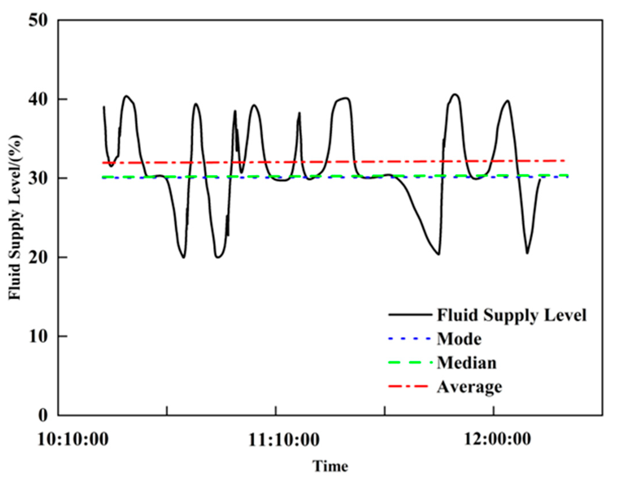
The level features of the low-production well time series data reflect the average state of the data over a period and are used to describe its overall stability level. The median, mode and mean are extracted as the level features of the liquid supply level. The median reflects the central value of the data but is less accurate when the distribution is uneven and its segment often coincides with the mode; by contrast, the mean varies with all data points and more comprehensively reflects the data level.

The results of the long-term level feature analysis for the liquid supply level are shown in Figure 22. When extracting short-term and long-term level features for the low-production well time series data, the mean is used comprehensively. Taking the liquid supply level as an example: when the mean is above the normal level, it indicates higher formation energy; when equal to the normal level, it indicates normal formation energy; when below the normal level, it indicates relatively low formation energy.

(2)

Trend feature extraction

The trend features of the low-production well time series data reflect the direction of change over a period and are an important basis for forecasting and planning in a time series analysis. Because the liquid supply level, dynamic fluid level, and production rate exhibit different trends at different time scales, short-term and long-term trend features must be extracted separately. The short-term trend can be characterized by the relative change rate, whose mathematical expression is as follows:

$$R={\displaystyle \frac{V_f-V_i}{V_i}}\times 100\%$$

(36)

In the formula, $R$ is the relative change rate; $V_f$ is the final value; $V_i$ is the initial value.

When the relative change rate is positive, the data show an upward trend, indicating high formation energy; when zero, the data remain unchanged, indicating normal energy; when negative, the data decline, indicating low formation energy. Because downhole conditions are complex, long-term time series data usually show irregular changes and it is necessary to compare different trend extraction methods; among them, the moving average method and the linear regression method are two commonly used methods. Using the liquid supply level data from Low-production Well-1 and Low-production Well-2 as examples, trend features were extracted, respectively, by the moving-average method (Formulas (37) and (38)) and the linear regression method (Formulas (39) and (40)).

$$y_1=-2.7586x_1+12$$

(37)

$$y_2=-0.1005x_2+44.8$$

(38)

$$y_3=-4.3845x_3+19$$

(39)

$$y_4=-3.4997x_4+15$$

(40)

In the formulas: $y_1-y_4$ is the liquid supply level; $x_1-x_4$ is time.

Table 8. Trend feature extraction methods.

Comparison Dimension	Moving Average Method	Linear Regression Method
Core Feature	Smoothes data to reduce fluctuations, suitable for short-term trend analysis	Fits data to describe trends, suitable for long-term trend analysis
Applicable Scope	Captures short-term fluctuations and rapidly changing trends	Identifies long-term trends and cyclical changing trends
Adapted Data Type	Data with stable or slight trends	Data with linear or approximately linear relationships
Outlier Stability	Relatively sensitive to outliers or noisy data	Relatively stable to outliers or noisy data
Parameter Flexibility	Parameters (e.g., window size) need to be adjusted according to data frequency and fluctuation	Linear fitting can well adapt to different data forms

summarizes the moving average method and the linear regression method for trend feature extraction and provides a comparative illustration of their core characteristics.

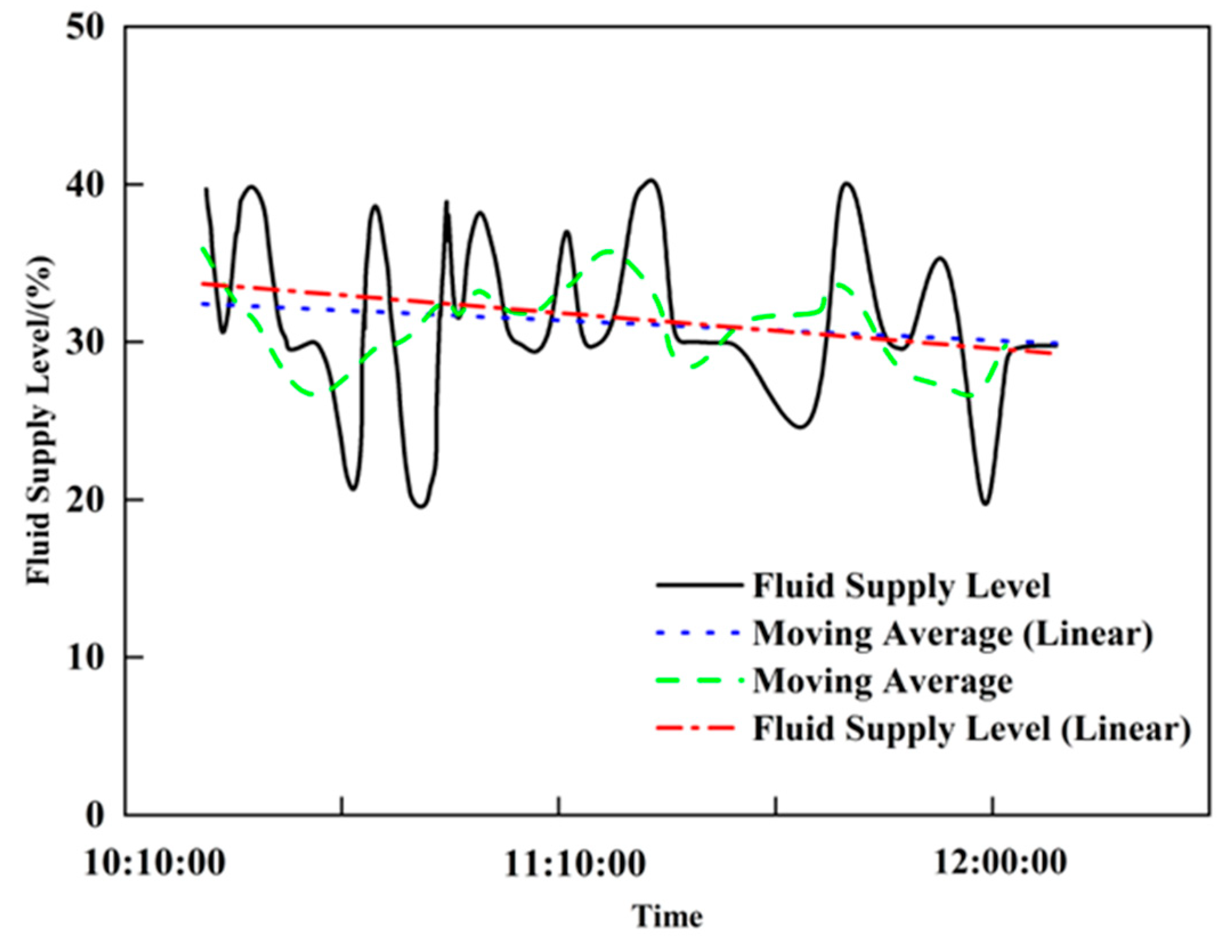
As shown in Figure 23 and Figure 24, the black solid line represents the Fluid Supply Level, the blue dashed line denotes the Moving Average (Linear), the green dash-dotted line indicates the Moving Average, and the red dash-dotted line stands for the Fluid Supply Level (Linear). The vertical axis represents the Fluid Supply Level (%), and the horizontal axis indicates Time, presenting the changes in the fluid supply level and the results of different trend extraction methods from 10:10:00 to 12:00:00. The moving average and linear regression methods for Low-production Well-1 (Figure 23) are negative, accurately reflecting the declining trend in the liquid supply level and indicating low formation energy; for Low-production Well-2 (Figure 24), the decline in the liquid supply level is larger, and the linear regression slope (−3.4997) is significantly greater in magnitude than the moving average slope (−0.1005), indicating that linear regression is more precise for trend feature extraction.

In summary, by comparing the moving average and linear regression methods and considering the long-term characteristics of the low-production well time series data, linear regression is preferred to extract the three features. Data change is reflected by the curve slope: a positive slope indicates high formation energy, zero slope indicates normal formation energy, and a negative slope indicates low formation energy.

(3)

Fluctuation feature extraction

The fluctuation features of the low-production well time series data reflect the amplitude and frequency of changes, revealing the instability and volatility of the data.

Table 9. Different fluctuation feature values for the liquid supply level of three low-production wells.

Low-Production Well	Standard Deviation	Variance	Range
1	12.676	144.861	40
2	6.906	45.866	40
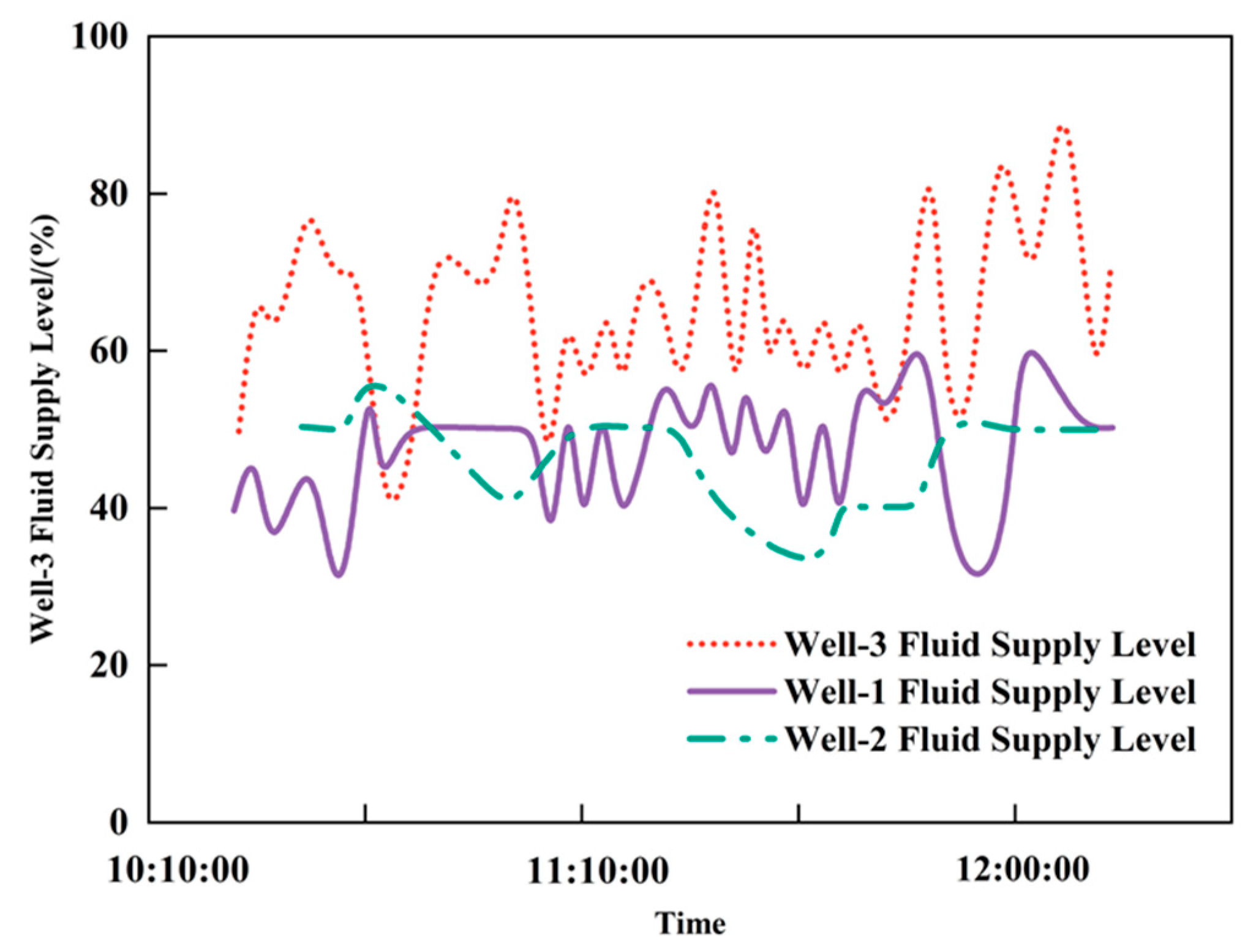
3	16.255	230.459	60

lists three extraction methods: standard deviation, variance and range. Taking the liquid supply level time series data from Low-production Wells-1, -2 and -3 as examples, the fluctuation features for the three wells are shown in Figure 25.

Figure 25 illustrates the fluid supply level trends of three wells over time: the red dotted line represents Well-3, the purple solid line denotes Well-1, and the green dash-dotted line indicates Well-2. The vertical axis stands for Fluid Supply Level (%), and the horizontal axis represents Time, presenting the dynamic fluid supply changes and capacity patterns of the three wells from 10:10:00 to 12:00:00, with the corresponding data shown in Table 9, the standard deviation, variance and range were calculated for the liquid supply level of Wells-1, -2 and -3. If the range is used, Well-3 shows the largest fluctuation while Wells-1 and -2 show the same fluctuation, which contradicts Figure 25, because the range only reflects the maximum and minimum values and ignores intermediate changes. Therefore, both standard deviation and variance can accurately reflect fluctuation, with the standard deviation being more intuitive and suitable as the fluctuation feature for liquid supply level.

Because the short-term window is brief, fluctuation features do not need to be extracted for the short term; only long-term fluctuation features are extracted for the low-production well time series data. When the standard deviation is above the normal fluctuation range, formation energy is relatively high; when within the normal range, formation energy is normal; when below the normal range, formation energy is relatively low.

(4)

Example of feature extraction

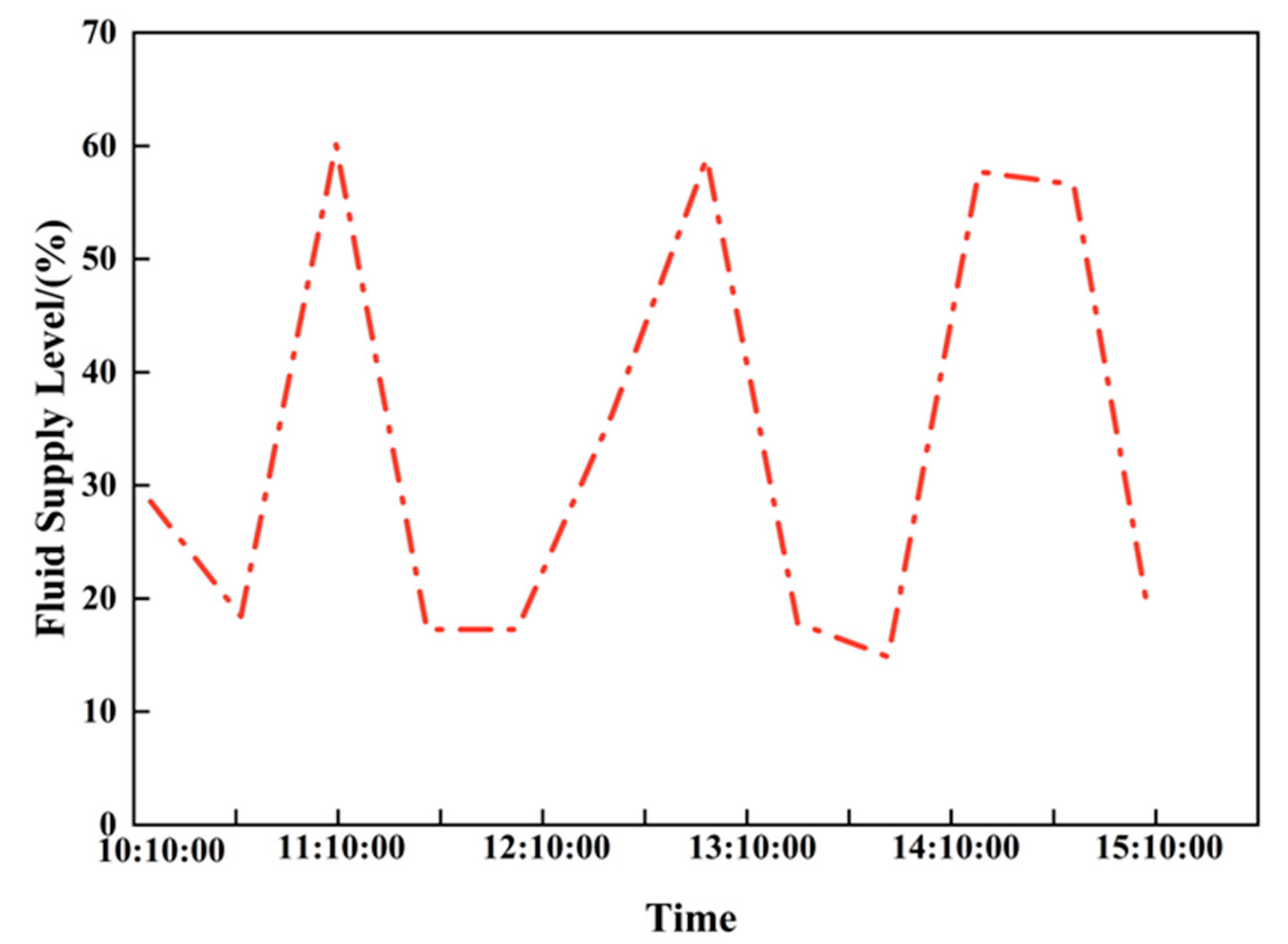
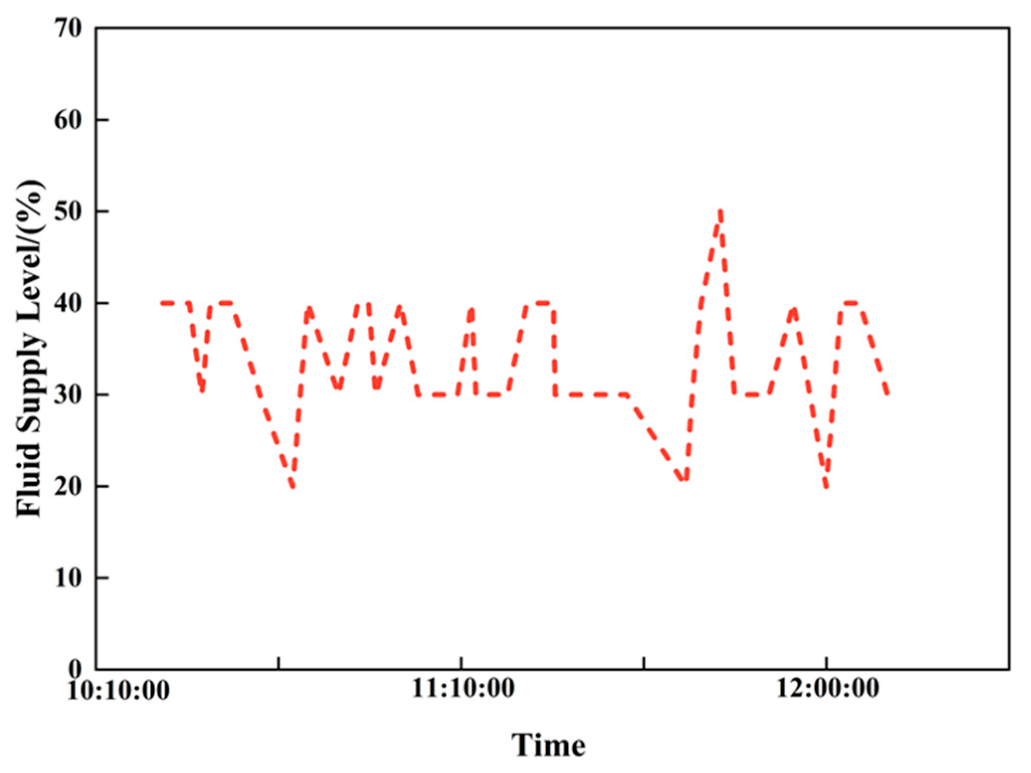
Time series data of the liquid supply level from an actual field are selected as the study index; the liquid supply level time series for the low-production well is shown in Figure 26. The normal level for this well is 61%, the normal trend is 0.018, and the normal fluctuation range is [6.68, 10.08].

As shown in

Table 10. Feature extraction for the liquid supply level time series of the low-production well.

Time Series Data Feature	Short-Term Time Window	Long-Term Time Window
Level/(%)	46.11	43.55
Trend	−1.33	−3.20
Fluctuation	/	8.77

, in the short-term time window, the well’s level is 46.11% with a trend change of −1.33; in the long-term window, the level is 43.55% with a trend change of −3.20 and a fluctuation of 8.77. The comprehensive feature analysis indicates that the well’s formation energy is relatively low and production parameter optimization is required.

3.4.2. Production Parameter Optimization for Low-Production Wells Based on the Analytic Hierarchy Process (AHP)

Most existing production parameter optimization methods for low-production oil wells rely on single-factor decision-making based on the fluid supply degree derived from dynamometer cards, making it difficult to comprehensively characterize the integrated dynamic changes in formation energy. To address this limitation, this study proposes a production parameter optimization method for low-production oil wells based on the Analytic Hierarchy Process (AHP).

This method constructs a weighted average comprehensive evaluation function to systematically integrate multi-dimensional indicators characterizing formation energy, including long-term and short-term fluid supply degrees, liquid production rate, and dynamic liquid level. It thereby realizes multi-index collaborative decision-making for production parameters and ultimately determines the optimal production parameter scheme based on the comprehensive decision results.

The optimization objective function is constructed with the core goal of “production improvement + energy consumption reduction”. Considering the production characteristics of low-production oil wells, such as limited fluid supply capacity and a relatively high proportion of energy consumption, this optimization abandons the single production-oriented decision-making logic and establishes a “production energy consumption” dual-objective optimization system. This system ensures an effective improvement in production capacity while achieving a significant reduction in energy consumption, with the mathematical expressions as follows:

$$\begin{array}{l}\max f_1(Q)=DailyOil\mathrm{Pr}oduction(q,s,n)\\ \min f_2(Q)=EnergyConsumptionperUnitOil\mathrm{Pr}oduction(q,s,n)\end{array}$$

(41)

Among them, q represents the displacement of the oil pump, s denotes the stroke length, and n is the pumping frequency. The core optimization logic is “maximizing daily oil production while minimizing the energy consumption per unit oil production under the premise of stable fluid supply”—which not only avoids problems such as equipment idle pumping and a sharp increase in energy consumption caused by blind production increase, but also solves the industry pain point of “high production without high efficiency” in low-production oil wells.

(1)

Comprehensive decision-making for long-term feature changes

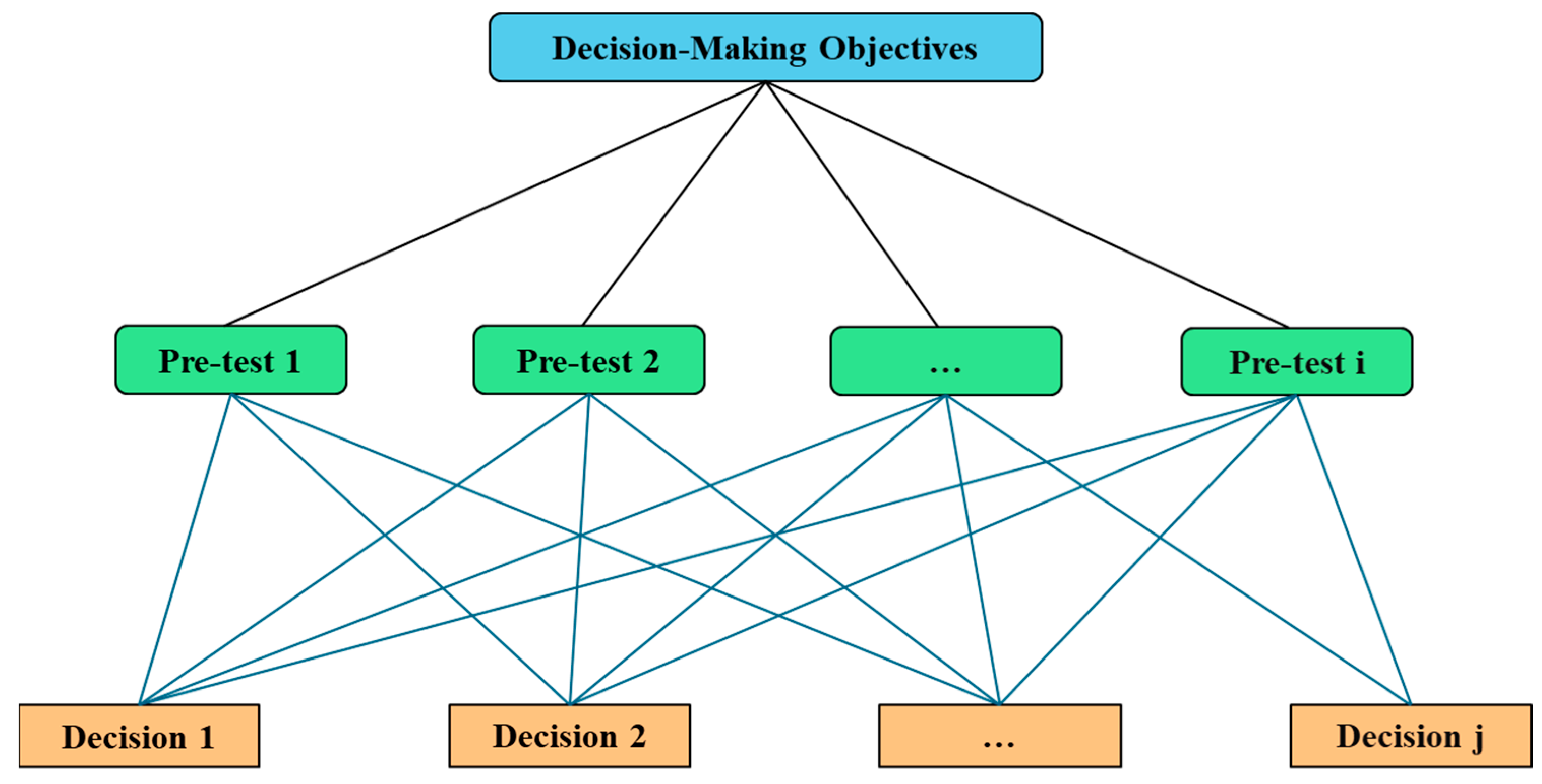
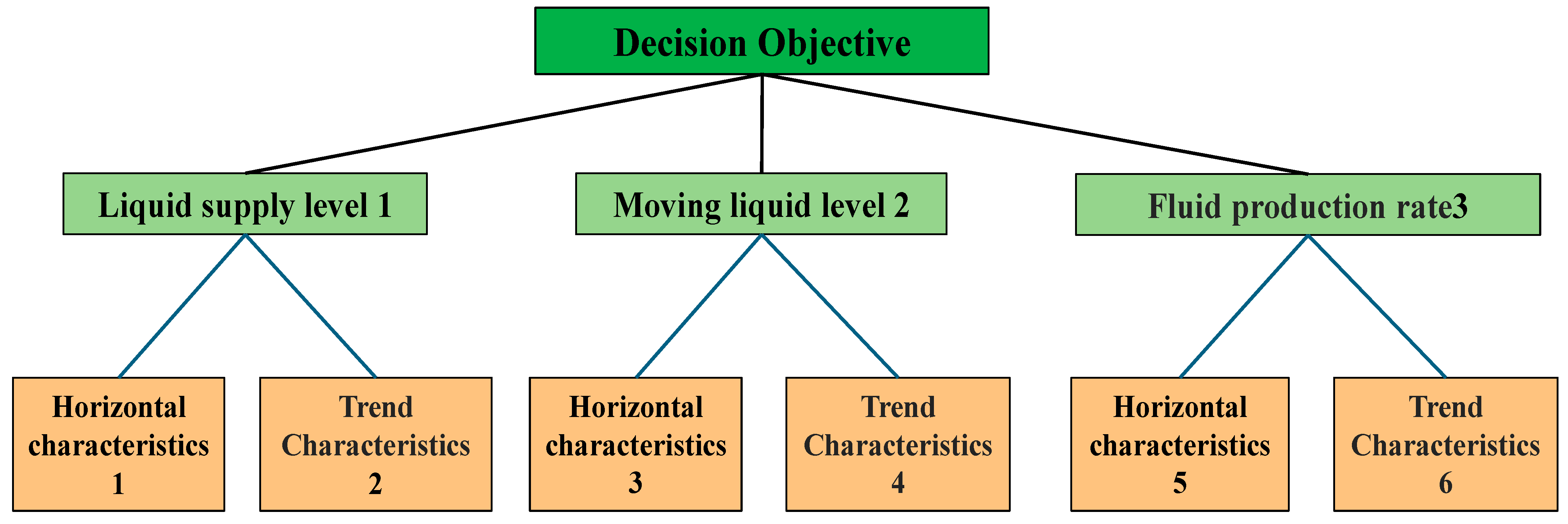
To optimize production parameters for low-production wells, level, trend and fluctuation features of liquid supply level, dynamic fluid level and production rate are first extracted from a long-term time window to provide the basis for optimization. Based on these features, a multi-level structural model for optimizing production parameters of low-production wells is established. The hierarchy for long-term production parameter optimization of low-production wells is shown in Figure 27.

The judgment matrix is created by pairwise comparisons of each element, typically using Saaty’s 1–9 scale; the specific comparison scale values are shown in

Table 11. Saaty’s 1–9 scale.

Scale Value	Meaning
1	Indicates the two elements are equally important
3	Indicates one element is slightly more important than the other
5	Indicates one element is noticeably more important than the other
7	Indicates one element is very strongly more important than the other
9	Indicates one element is extremely more important than the other
2, 4, 6, 8	Intermediate values between the two adjacent judgments. For example, 2 is more important than 1 but less important than 3

.

Construct the judgment matrices and perform pairwise comparisons of the features using Saaty’s 1–9 scale (Table 11) to determine relative importance and then compute the weights of each time series feature with respect to the decision objective (

Table 12. Long-term criterion-level judgment matrix.

	Production Rate	Dynamic Fluid Level	Liquid Supply Level
Production rate	1	0.333	0.25
Dynamic fluid level	3	1	0.5
Liquid supply level	4	2	1

and

Table 13. Long-term Decision-Making Layer Judgment Matrix.

Feature Type	Fluctuation Characteristic	Trend Characteristic	Level Characteristic
Fluctuation Characteristic	1	0.5	2
Trend Characteristic	2	1	3
Level Characteristic	0.5	0.333	1

).

Next, single-level ranking and consistency checks are carried out, yielding the ranking weight vector $W_C={[0.567,0.411,0.119]}^T$, ${\lambda }_{\max }=3.107$; the consistency check produces: $CI=0.021$, $RI=0.58$, $CR=0.054<0.1$, and the judgment matrix passes the consistency test. Using the above steps, the weight vector:

$W_D={[0.158,0.490,0.302,0.159,0.535,0.312,0.146,0.487,0.324]}^T$. Then, an overall hierarchical ranking and consistency check are performed: based on the already determined weights of the criterion layer relative to the goal and the weights of the decision layer relative to the criterion layer, the overall hierarchical ranking

$Y={[0.087,0.289,0.157,0.048,0.169,0.086,0.016,0.059,0.043]}^T$, $CR=0.019<0.1$ is obtained, and the judgment matrices pass the consistency checks.

Finally, compute the comprehensive decision result from the overall hierarchical ranking and consistency checks using the criterion-to-goal and decision-to-criterion weights, thereby constructing the long-term feature comprehensive decision model. The corresponding results are detailed in the overall summary table in the subsequent section.

(2)

Comprehensive decision-making for short-term feature changes

To optimize production parameters for a low-production well, level, trend and fluctuation features of the liquid supply level, dynamic fluid level and production rate are first extracted from a short-time window to provide the basis for optimization. Based on these features, a multi-level structural model for optimizing production parameters of low-production wells is established. The hierarchical structure for short-term optimization is shown in Figure 28.

Construct judgment matrices and perform pairwise comparisons of the features using Saaty’s 1–9 scale (Table 11) to determine relative importance, and from these, compute the weights of each time series feature with respect to the decision objective (

Table 14. Short-term decision-level judgment matrix trend feature.

	Level Feature	Level Feature
Level feature	1	2
Level feature	0.5	1

).

Next, single-level ranking and consistency checks are performed, yielding the ranking weight vector $W_C={[0.567,0.411,0.119]}^T$, ${\lambda }_{\max }=3.107$. The consistency check gives $CR=0.054<0.1$, and the judgment matrix passes the consistency test.

Using the above steps the weight vector $W_D={[0.291,0.598,0.291,0.598,0.291,0.598]}^T$ is calculated. Then perform overall hierarchical ranking and consistency checks: based on the already determined weights of the criterion layer relative to the goal and the decision layer relative to the criterion layer, compute the overall weights: $Y={[0.179,0.369,0.110,0.224,0.050,0.079]}^T$. The consistency yields $CR=0.027<0.1$, indicating the pairwise comparison matrix passes the consistency test. Finally, construct the short-term feature comprehensive decision model; the results are shown in

Table 15. Comprehensive Decision-Making for Long-Term, Short-Term, and Overall Feature Changes Based on the Analytic Hierarchy Process (AHP).

Comprehensive Decision Factor	[−1, −0.5)	[−0.5, 0.5]	(0.5, 1]
Long-term feature changes	Negative adjustmen	No adjustment	Positive adjustment
Short-term feature changes	Negative adjustmen	No adjustment	Positive adjustment
Overall feature range	Negative adjustmen	No adjustment	Positive adjustment

.

(3)

Comprehensive decision-making for combined long- and short-term features

Long-term feature changes reflect the long-term rising or falling trend of low-production well time series data, while short-term feature changes reflect short-term sudden changes and instability; the two are related in the data. Therefore, in production parameter optimization for low-production wells, short-term comprehensive decisions are integrated with long-term trend comprehensive decisions to form a combined long- and short-term decision. The calculation formula is as follows:

$$CM=\epsilon \left[f\left(H_1,T_1,L_1\right)+f\left(H_2,T_2\right)\right]$$

(42)

In the formula, $CM$ is the combined decision factor for long- and short-term features; $\epsilon$ is the time weight coefficient ($\epsilon$ = 0.5); $f\left(H_1,T_1,L_1\right)$ is the long-term feature decision function; $f\left(H_2,T_2\right)$ is the short-term feature decision function; $H$ is the level feature; $T$ is the trend feature; $L$ is the fluctuation feature.

The AHP-based overall feature comprehensive decision results are shown in Table 15.

According to the earlier single-factor decision example analysis, single-factor decisions have limitations in consistency and scientific validity: some decision factors need adjustment while others do not. Therefore, to achieve a scientifically reasonable optimization of production parameters for low-production wells, a comprehensive decision method is necessary.

From the above calculations, the combined weight of long-term features was determined to be ${[0.087,0.289,0.157,0.048,0.169,0.086,0.016,0.059,0.043]}^T$, with the long-term decision factor equal to −0.613.

Meanwhile, the short-term feature weight is ${[0.179,0.369,0.110,0.224,0.050,0.079]}^T$. Using the formula for combined long- and short-term decision-making, the resulting comprehensive decision factor is $MC=0.5\times \left(-0.613-0.419\right)=-0.516$.

The comprehensive decision result falls within the negative adjustment interval $[-1,-0.5)$, clearly indicating that a negative regulation of the pumping frequency of the low-production oil well should be implemented in the current time period. The core of this decision-making logic lies in moderately reducing the pumping frequency to dynamically match the pumping parameters with the formation fluid supply capacity, thereby avoiding idle pumping losses caused by blind production increase and ultimately achieving the coordinated optimization of the oil well’s production efficiency and energy consumption economy.

4. Conclusions

(1)

Aiming at the problem that the LSTM network structure does not match the data characteristics of the low-yield well indicator card, the LSTM prediction model of the low-yield well indicator card is constructed based on the actual well conditions and LSTM characteristics. Compared with the commonly used BP neural network and RNN model, the model performs better in prediction performance, and the average prediction performance index Q is 0.08.

(2)

A CNN was used to extract and analyze the liquid supply level data from dynamometer cards of low-production wells, verifying the applicability of CNNs for identifying liquid supply capacity from dynamometer cards. Case results show identification accuracies exceeding 98%, enabling effective prediction-matching of dynamometer cards and accurate extraction of the liquid supply level information.

(3)

For the representation relationship among three types of time series data—the liquid supply level, dynamic fluid level, and production rate—and formation energy, a multi-indicator fusion method for production parameter optimization was proposed. Using liquid supply level, dynamic fluid level and production rate as core indices, level, trend and fluctuation features were extracted and combined with AHP to construct a comprehensive decision model (CR < 0.1), achieving standardized control of production parameters.

(4)

Based on the representation relationships among liquid supply level, dynamic fluid level and production rate and formation energy, a closed-loop system of “data preprocessing—condition prediction—state identification—parameter optimization” was constructed. This system integrates LSTM, CNN and AHP modules and ensures data quality through standardized processing. Field application results show the system can predict dynamometer cards in advance, accurately identify liquid supply fluctuations, and output optimization schemes, effectively achieving intelligent operation and maintenance of low-production wells.

(5)

This study has two limitations: first, the model training data are derived from a single block and have not been validated in oilfields with different geological conditions, so its generalization performance remains to be tested; second, the current parameter optimization only targets pumpjack frequency and does not involve the coordinated optimization of multiple parameters such as stroke length and stroke rate. Future research can be expanded in two aspects: first, introducing key dynamic formation parameters such as real-time reservoir pressure and dynamic fluid supply capacity to enhance the dynamic adaptability between production parameters and formation conditions; second, integrating intelligent algorithms such as reinforcement learning to construct a closed-loop dynamic optimization model based on real-time feedback, realizing the adaptive iterative adjustment of production parameters.