A TCN-BiGRU Density Logging Curve Reconstruction Method Based on Multi-Head Self-Attention Mechanism

Abstract

In the process of oil and natural gas exploration and development, density logging curves play a crucial role, providing essential evidence for identifying lithology, calculating reservoir parameters, and analyzing fluid properties. Due to factors such as instrument failure and wellbore enlargement, logging data for some well segments may become distorted or missing during the actual logging process. To address this issue, this paper proposes a density logging curve reconstruction model that integrates the multi-head self-attention mechanism (MSA) with temporal convolutional networks (TCN) and bidirectional gated recurrent units (BiGRU). This model uses the distance correlation coefficient to determine curves with a strong correlation to density as a model input parameter and incorporates stratigraphic lithology indicators as physical constraints to enhance the model’s reconstruction accuracy and stability. This method was applied to reconstruct density logging curves in the X depression area, compared with several traditional reconstruction methods, and verified through core calibration experiments. The results show that the reconstruction method proposed in this paper exhibits high accuracy and generalizability.

1. Introduction

In oil and gas exploration and development, logging data play a crucial role in revealing the physical properties of rocks and the characteristics of reservoir fluids. However, in practical applications, factors such as instrument failures and wellbore enlargement often lead to distortion or loss of some logging data, posing challenges for subsequent comprehensive evaluations of oil and gas reservoirs [1,2]. Re-logging is not only costly but also technically challenging for wells that have been cemented. Therefore, exploring methods to reconstruct missing or distorted logging curves are significant for detailed logging interpretation.

Due to the inherent correlations between different logging curves, when instrument failure results in missing curves, the missing curves can be inferred from the data correlations of the other intact curves. If borehole enlargement affects the measurements, the curves less affected by the enlargement can be used to infer the more affected curves. Therefore, two reconstruction methods were developed in early studies: one is based on empirical formulae established through experimental statistics, such as the Faust formula, which establishes the relationship between formation acoustic velocity and resistivity, and the Gardner formula, summarizing the relationship between sound speed and density [3]. However, these formulae require conditional constraints and involve researchers’ subjective considerations, which make them unsuitable for complex strata [4]; another method is based on the latent correlation among curves, using the multivariate fitting method (MCF) to establish a response equation between logging curves and the target reconstruction curve, which somewhat avoids the subjective influence of empirical formulae. However, complex geological actions result in lateral and vertical heterogeneities of strata, and most logging response characteristics are non-linear, leading to low accuracy in the curves fitted by the second method [5].

With the rapid development of computer technology, the integration of machine learning and deep learning with multidisciplinary fields has provided new insights for logging curve reconstruction. Employing shallow machine learning algorithms to fit the complex non-linear relationships between curves is the simplest data-driven method [6]. However, due to their simple network structures and poor non-linear fitting capabilities, these shallow algorithms have limited applicability in complex geological scenarios. Deep learning, an important method evolved from machine learning, features self-organization, self-learning, and non-linear dynamic processing [7]. With simple data training, deep learning can fit high-dimensional mapping relationships layer by layer. Thus, more and more experts and scholars attempt to use deep learning technologies to solve issues of distorted or missing curves. You et al. [8] proposed a capillary pressure curve reconstruction technique based on the back propagation (BP) neural network and achieved good results. Mo et al. [9] introduced a reconstruction method based on a genetic neural network, which overcomes the traditional network’s drawback of falling into local minima and achieves high accuracy in reconstructing sonic, density, and resistivity curves. However, these networks mainly focus on the functional relationships between curves without considering the temporal relationships between strata layers. Therefore, some scholars have proposed more refined curve reconstruction methods based on improved recurrent neural networks (RNN) to enhance the accuracy of logging curve reconstruction [10,11,12,13,14,15,16]. With the continuous development of deep learning, convolutional neural networks (CNN) have achieved remarkable results in fields like image recognition, being capable of extracting adjacent parameter features and uncovering the correlations among different logging data [17,18,19,20,21]. Many experts and scholars have actively attempted to incorporate CNN into curve reconstruction and have also achieved good effects. Lei Wu et al. proposed a combined model of CNN and LSTM (long short-term memory) which extracts the spatiotemporal features of logging data and uses the particle swarm optimization algorithm (PSO) to determine the optimal hyperparameters of the CNN-LSTM structure, significantly reducing optimization time in complex strata. Duan et al. [22] utilized a model that combines CNN and GRU (gated recurrent unit) and employed a conditional generative adversarial nets (CGAN) adversarial training method to extract non-linear correlations between curves more effectively. Jun Wang et al. [23] introduced a model that combines convolutional neural networks and bidirectional gated recurrent unit (BiGRU) with the attention mechanism, enhancing curve reconstruction accuracy by extracting local features with the CNN module and capturing the depth variation trends of logging data with the BiGRU module. However, these integrated models are prone to gradient vanishing and exploding issues, and they have low computational efficiency and a tendency for overfitting.

2. Methodology

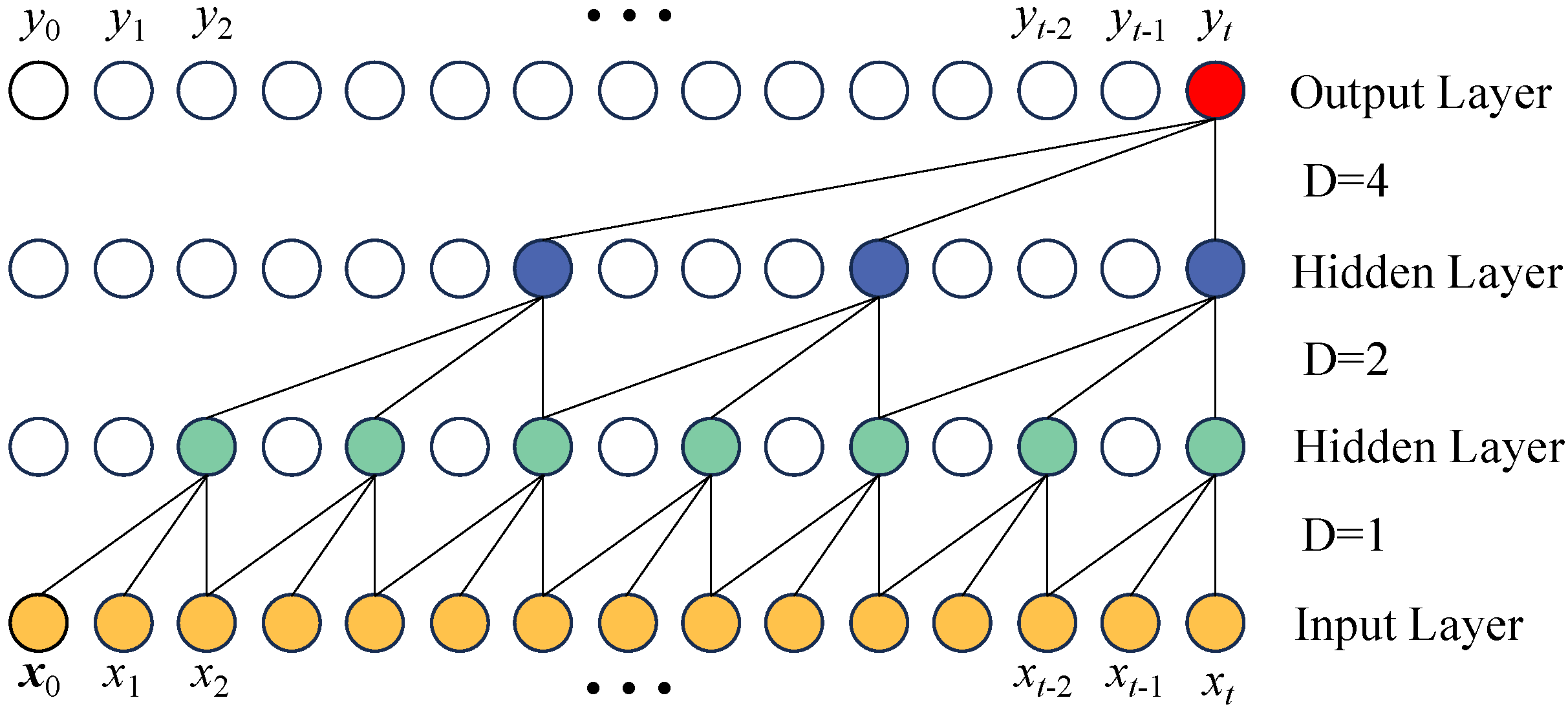
2.1. Temporal Convolutional Networks

Temporal convolutional networks (TCN) represent an improved network that combines the advantages of RNNs and CNNs [24]. By integrating causal convolutions with dilated convolutions and incorporating residual connections (residual network), TCNs address the deficiencies of CNNs in capturing long-term dependencies in time-series data and maintaining causality. They effectively mitigate issues related to gradient vanishing and exploding, enabling TCNs not only to mine high-dimensional features and temporal relationships within data efficiently but also to achieve more stable gradients and a more flexible receptive field with reduced memory usage. This offers significant advantages in multivariate time-series analysis [25,26,27].

2.1.1. Dilated Causal Convolution

Causal convolution guarantees that the output at a given time (t) is influenced solely by the input at time t and preceding moments in subsequent layers, thus creating a forward temporal relationship in time-series analysis. Meanwhile, dilated convolution broadens the receptive field of the neural network through intervallic sampling of the input using a dilation rate, enabling the capture of longer-distance data dependencies without increasing the number of parameters or computational complexity. As shown in Figure 1, with a dilation rate D = 4, every fourth sampling point is used as an interval for sampling. This approach ensures an expanded receptive field while minimizing the number of parameters.

Figure 1. Dilated causal convolution structure. The yellow circles represent the input curve sequence features processed by this module. The span encompassed by the convolution kernel is marked by the shift from green to blue. A dilation rate D = 4 signifies that every fourth point is sampled.

2.1.2. Residual Module

Experience shows that increasing the depth of neural networks can enhance their ability to process non-linear data, yet deep networks may encounter issues such as gradient vanishing or exploding. To address these problems, we introduced the concept of residual networks [28]. By keeping the filter size (k) and dilation factor (D) constant, incorporating a residual network can expand the network’s receptive field and enable deeper training levels. Each convolution layer utilizes a generic residual module, as depicted in Figure 2. This module’s structure consists of two sets of dilated non-causal convolutions, weight normalization, ReLU activation function, and a dropout layer, forming the function definition.

$$X^{i+1}=Activation(X^i+F\left(X^i\right)).$$

(1)

Figure 2. Residual module structure. The diagram features two dilated causal convolution layers using a kernel size k and dilation factor d, interleaved with ReLU and dropout layers, and a 1 × 1 convolution responsible for dimension matching.

In this context, $X^i$ denotes the input fed into the residual module, whereas $X^{i+1}$ signifies the resultant output, with the term “Activation” designating the activation unction utilized.

2.2. Bidirectional Gated Recurrent Unit

Recurrent neural networks (RNNs) are capable of memorizing previous inputs, making them well suited for processing time-series data and particularly effective at extracting temporal features from curves [29]. Nevertheless, conventional RNNs are hindered by issues related to the vanishing or exploding of gradients, thereby constraining their ability to retain long-term memory. To overcome the dependency issues of RNNs, Chuang J et al. introduced the gated recurrent unit (GRU) in 2014 [30]. This network adds additional update gates and reset gates in each recurrent unit to control the inputs, which allow the network to maintain state information over longer time periods. The GRU unit structure, as shown in Figure 3, operates according to the following formulae:

$$z_t=\sigma (W_{iz}{x}_t+b_{iz}+W_{hz}{h}_{t-1}+b_{ht}).$$

(2)

$$r_t=\sigma (W_{ir}{x}_t+b_{ir}+W_{hr}{h}_{t-1}+b_{hr}).$$

(3)

$${\tilde{h}}_t=tanh\left(W_{in}{x}_t+b_{in}+r_t\odot (W_{hn}{h}_{(t-1)}+b_{hn})\right).$$

(4)

$$h_t=(1-z_t)\odot h_{(t-1)}+z_t\odot {\tilde{h}}_t.$$

(5)

Here, $h_{t-1}$ represents the hidden state from the previous moment, $x_t$ denotes the current input, and $\sigma$ stands for the sigmoid activation function; $r_t$ is the reset gate, and $z_t$ represents the update gate; ${\tilde{h}}_t$ is the candidate hidden state, and $h_t$ indicates the final hidden state; W is the weight matrix, ⊙ denotes the Hadamard product, and b refers to the bias parameters.

Figure 3. Structure of GRU unit.

The bidirectional gated recurrent unit (BiGRU) is formed by GRUs in two orientations, processing time-series data in opposing directions through a dual-layer GRU network. Each direction is designated to handle either historical or future information [31,32]. The structure is illustrated in Figure 4. This bidirectional framework enables the BiGRU to capture information within the data more comprehensively, thereby enhancing the reconstruction performance of the model.

Figure 4. Structure of BiGRU network.

2.3. Multi-Head Self-Attention Mechanism

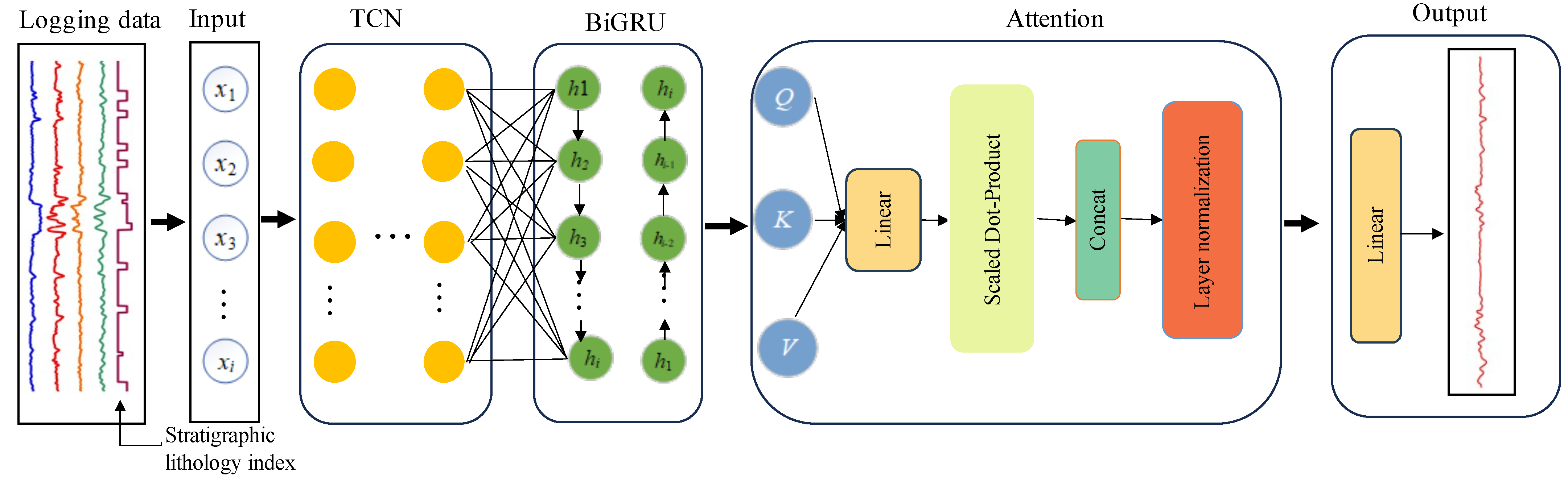
The attention mechanism was first introduced by Bahdanau et al. [33] in the field of neural machine translation, enhancing the model’s ability to focus on key information through weighted allocation. Different logging curves exhibit significant variations in their characteristic responses to the same rock formation. The multi-head self-attention mechanism is capable of assessing the impact of input features on the reconstructed curves and assigning corresponding weights to each feature. This highlights information significantly affecting the reconstructed curve, thereby improving model accuracy. The structure of this mechanism is illustrated in Figure 5. It learns the data’s multifaceted relationships through multiple independent focal points and utilizes a structure with h heads that are mapped to query, key, and value spaces, forming three parameter matrices: $Q_i$, $K_i$, and $V_i$ The computation process for each attention head is as follows.

Figure 5. Multi-head self-attention mechanism structure. It includes Q for query, K for key, and V for value, all of which are transformations of the same input feature.

First, multiply the input with h sets of parameter matrices $W_Q$, $W_K$, and $W_V$ to obtain the Query matrix Q, Key matrix K, and Value matrix V:

$$Q_i=X{W}_{Qi},K_i=X{W}_{Ki},V_i=X{W}_{Vi}.$$

(6)

Here, i represent the i attention head, and X is the input.

Second, apply the scaled dot-product attention scoring function to each attention head’s query, key, and value to calculate the attention scores A:

$$A_i=\mathrm{softmax}\left({\displaystyle \frac{Q_i{K}_i^T}{\sqrt{d_k}}}\right)V_i.$$

(7)

Here, $d_k$ is the dimension of the attention head; the softmax function produces attention weights.

Finally, concatenate the outputs of the h attention heads together and project them through a parameter matrix $W_O$ to obtain the final output:

$$\mathrm{MultiHead}\left(X\right)=\mathrm{Concat}(A_1,\dots ,A_h)W_O.$$

(8)

2.4. TBMSA

In practical well logging, the sampling intervals of data are notably short, yet the interlayer influence between strata at different depths can span 30 to 50 m. This indicates that the reconstruction of logging curves involves the analysis of sequential data with long-term bidirectional correlations [34], making the TBMSA model particularly apt for such challenges. The dilated causal convolution structure of TCNs enables the capture of dependencies over longer sequence distances with higher accuracy in logging curve reconstruction. Since the data recorded during logging do not represent the true value at the current depth but are instead a combined result of the current depth and the surrounding rock formations, the capability of the Bi-GRU network to process both forward and backward sequence data enhances the model’s ability to discern stratum features from both past and future time series, thus effectively mining for hidden information. The correlation among different logging curves varies significantly; introducing a multi-head self-attention mechanism that assigns weights to input data can, to some extent, mitigate the shortcomings of BiGRU in extracting critical information [35,36].

The TBMSA framework is depicted in Figure 6. Initially, lithology records and logging curve information are preprocessed and merged to form the model’s input. Initial feature extraction is conducted through TCN and preserving information across the temporal dimension. This is followed by initial feature extraction through TCN and information on the temporal dimension is retained. Subsequently, BiGRU receives the data sequence processed by TCN. Its bidirectional structure allows for a more comprehensive exploration of the temporal relationships in logging data and a capture of the correlational properties of the strata above and below. The attention module quantifies the feature weights of the data outputted by BiGRU and further learns the correlations among logging data.

Figure 6. TBMSA model structure diagram. The input data, composed of well logging data combined with stratigraphic lithology indicators, passes through TCN, BiGRU, and attention modules before outputting the reconstructed density curve.

Ultimately, the attention module assigns weights to the data, which are then funneled through a fully connected layer for the purposes of extracting features and reducing dimensions. This process results in the generation of the reconstructed curve’s output.

2.5. Model Evaluation Metrics

This research utilizes mean squared error (MSE), root mean squared error (RMSE), and mean absolute error (MAE) to assess the model’s performance. The equations for these evaluation measures are provided below:

$$\mathrm{MSE}={\displaystyle \frac{1}{n}}\sum _{i=1}^n{(y_i-{\widehat{y}}_i)}^2.$$

(9)

$$\mathrm{RMSE}=\sqrt{{\displaystyle \frac{1}{n}}\sum _{i=1}^n{(y_i-{\widehat{y}}_i)}^2}.$$

(10)

$$\mathrm{MAE}={\displaystyle \frac{1}{n}}\sum _{i=1}^n\left|y_i-{\widehat{y}}_i\right|.$$

(11)

Within the equations, n signifies the aggregate count of samples, $y_i$ corresponds to the genuine curve data, and ${\widehat{y}}_i$ is indicative of the data from the reconstructed curve. The smaller the value of MSE and RMSE, the stronger the model’s generalization ability and stability; similarly, the smaller the value of MAE, the better the model’s fitting effect.

3. Case Study

The experimental data for this study were derived from actual well logging information from four wells located within an exploration and development area in the West Lake depression. The data for these wells encompass a range of curves, including caliper (CAL), neutron porosity (CNCF), acoustic slowness (DT), density (DEN), natural gamma ray (GR), and spontaneous potential (SP). The detection depth spanned from 2400 to 4200 m, with a sampling interval of 0.1 m. The logging data for these wells are complete, with only certain well segments showing distortion due to borehole enlargement. All selected datasets originate from the same target strata of the Paleogene system to ensure lateral consistency in the dataset characteristics. To validate the model’s ability to reconstruct logging data, we assume distortion or absence in the DEN curve. The curve reconstruction experiment is conducted using logging curve data from the four wells based on the TCN-BiGRU-MHA model, and we analyzed the capability of different methods to reconstruct logging curves based on the experimental results.

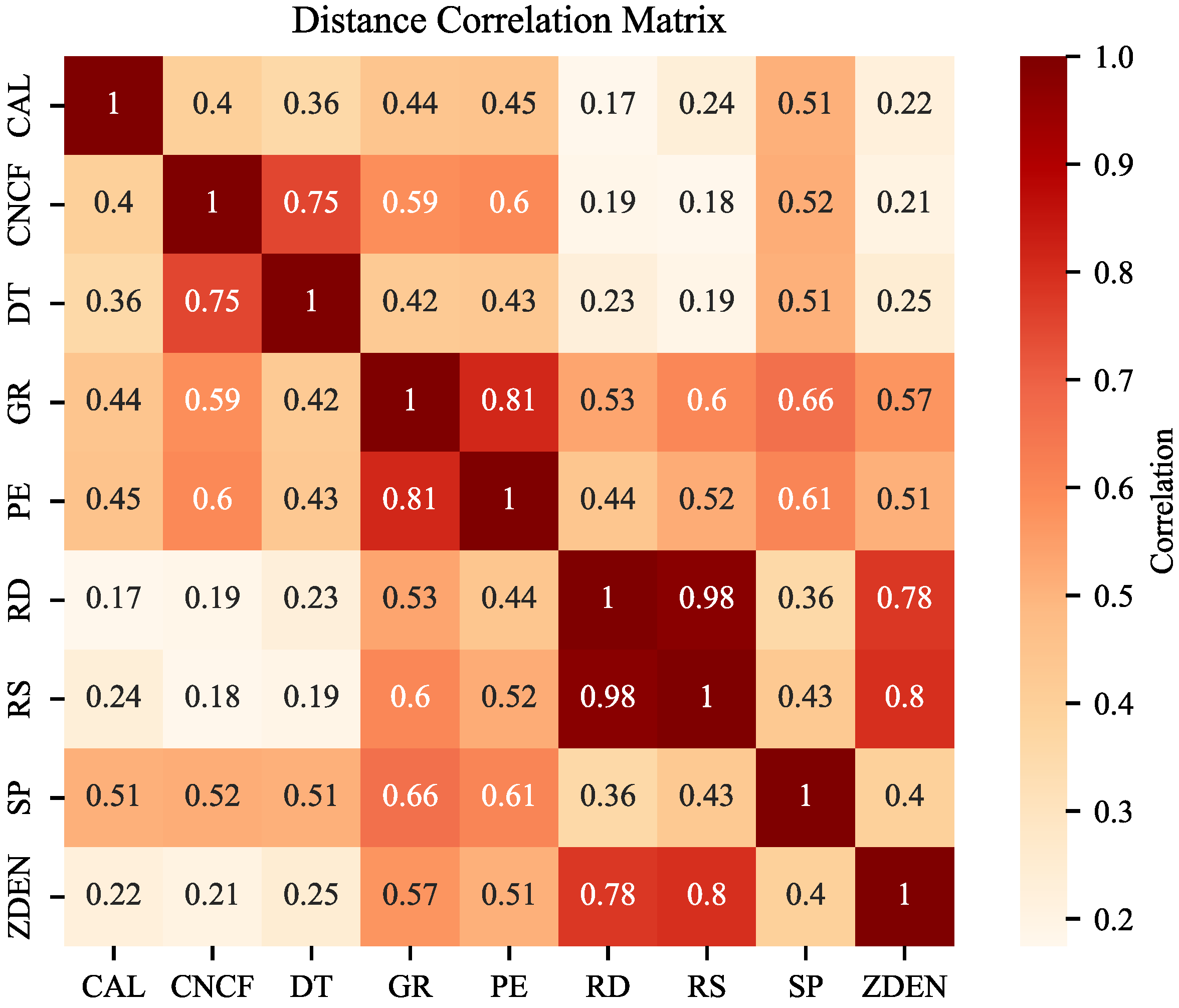
3.1. Correlation Analysis

To ascertain the integrity and applicability of the input data, a meticulous correlation analysis of the logging curves is indispensable. Consequently, this investigation leverages the distance correlation coefficient to rigorously examine the linear and non-linear interdependencies existing between the curves. This correlation coefficient relies on the distances between sample points rather than specific values, meaning it can capture the distribution and relative positions of the sample points, which include the structure of non-linear relationships. Taking two curve data, X and Y, as examples, their corresponding distance matrices are A and B. Double centering of distance matrices A and B yields $\tilde{A}$ and $\tilde{B}$, with their elements defined by the following formula:

$${\tilde{a}}_{ij}=a_{ij}-{\overline{a}}_i-{\overline{a}}_j+{\overline{a}}_v,$$

(12)

$${\tilde{b}}_{ij}=b_{ij}-{\overline{b}}_i-{\overline{b}}_j+{\overline{b}}_v$$

(13)

where ${\overline{a}}_i$ represents the mean of the $i^{th}$ row in matrix A, ${\overline{a}}_j$ denotes the mean of the jth column, and ${\overline{a}}_v$ is the general average across all elements. Using the above definitions, the distance covariance $dCov(X,Y)$, as well as the distance variances $dVar\left(X\right)$ and $dVar\left(Y\right)$, can be calculated.

$$dCov(X,Y)=\sqrt{{\displaystyle \frac{1}{n^2}}\sum _{i=1}^n\sum _{j=1}^n{\tilde{a}}_{ij}{\tilde{b}}_{ij}}$$

(14)

$$dVar\left(X\right)=\sqrt{{\displaystyle \frac{1}{n^2}}\sum _{i=1}^n\sum _{j=1}^n{\tilde{a}}_{ij}^2}$$

(15)

$$dVar\left(Y\right)=\sqrt{{\displaystyle \frac{1}{n^2}}\sum _{i=1}^n\sum _{j=1}^n{\tilde{b}}_{ij}^2}$$

(16)

Ultimately, the distance correlation coefficient $dCov(X,Y)$ is determined by employing Equation (17).

$$dCor\left(Y\right)={\displaystyle \frac{dCov(X,Y)}{\sqrt{dVar\left(X\right)·dVar\left(Y\right)}}}$$

(17)

In the formula, n represents the length of each column, and $dCor(X,Y)$ is the correlation coefficient between curve X and curve Y, with a range from 0 to 1. Here, 1 indicates perfect correlation, while 0 signifies no correlation at all.

Figure 7 shows the distance correlation calculation results among nine conventional logging curves in well A. It is observed that the curves with a correlation greater than 0.35 with the DEN curve include GR, PE, RD, RS, and SP. Moreover, the correlation between RD and RS is 0.98, which indicates that the two resistivity curves provide highly overlapping feature information. Therefore, GR, PE, SP, and RS are selected as input data for the experiment.

Figure 7. Heat map of correlation coefficient matrix for test wells where input data are CAL, CNCF, DT, GR, PE, RD, RS, and SP and target data are density (ZDEN).

3.2. Physical Constraint Analysis

Previous approaches to curve reconstruction based on deep learning primarily relied on the curve data itself and overlooked the importance of prior knowledge. To leverage existing data resources fully, this model incorporates stratigraphic lithology indicators (STRLIT) as physical constraints on top of the well logging curve data.These data are primarily derived from logging cuttings information, which is easily obtainable and provides the advantage of acquiring long continuous sections of labels. Different lithologies have distinct mineral compositions and pore structures, which manifest as fluctuations in numerical values on logging curves. By digitally labeling various lithology types for training (as shown in Table 1), the model can learn the patterns of curve variations with changes in lithology and then enhance the accuracy of model reconstruction.

Table 1. Lithology labels.

Lithology	Minerals	Tags
fine sandstone	quartz, dark minerals	1
siltstone	quartz	2
muddy siltstone	quartz, clay	3
mudstone	clay	4
siltstone	clay, quartz	5

To validate that incorporating physical constraints can enhance the model’s sensitivity to variations in logging curves, two models were compared in an experimental setup: one with physical constraints, the C-SA-TBMSA model; and another without, the USA-TBMSA model. It is assumed that the section from 2530 to 2930 m in Well A is the training data and the section from 2930 to 2980 m is the test set. The results of the model’s reconstruction and corresponding errors are presented in Figure 8 and Table 2. As shown in Figure 8, the reconstruction, represented by the fifth red line, is generated by the model incorporating physical constraints, whereas the actual curve is represented by the black line. Results of the model’s reconstruction and corresponding errors are showcased in Figure 8 and Table 2, with the red line in the sixth track symbolizing the model’s reconstructed curve that incorporates physical constraints, and the black line representing the actual curve. In the seventh track, the blue line demonstrates the reconstruction performed by the model without physical constraints. Analysis of Figure 8 and Table 2 reveals that both the CTBMSA and UTBMSA models have successfully reconstructed the logging curves, maintaining trends that align with those of the original curves. However, the CTBMSA model’s reconstruction exhibits lower error rates when compared to the original curve, achieving a reduction in MAE and RMSE of 24.1% and 17.1%, respectively, compared to the UTBMSA model. This indicates that the C-SA-TBMSA model has better reconstruction accuracy and stability, demonstrating the rationality of incorporating physical constraints into the model.

Figure 8. Comparison of the impact of physical constraints. The input data for the CTBMSA model with physical constraints include STRLIT, GR, RS, PE, and SP. For the UTBMSA model without physical constraints, the input comprises STRLIT, GR, RS, PE, and SP, all with data values of −3. The black curve represents the actual measured density curve, while the red and blue curves depict the reconstructed curves by CTBMSA and UTBMSA, respectively.

Table 2. The impact of physical constraints on the analysis of errors.

Model	MSE	RMSE	MAE
CTBMS	0.0038	0.0613	0.0371
UTBMS	0.0055	0.0739	0.0489

3.3. Comparative Experimental Analysis

3.3.1. Model Parameter Settings

To test the TBMSA model’s capability in reconstructing logging curves, a segment from Well B spanning 2600–2900 m was selected as the training set, 2900–3070 m as the validation set, and 2400–2550 m as the testing set. The chosen curves and stratigraphic lithology indicators were normalized and standardized before conducting the density curve reconstruction experiment. The proposed model’s reconstruction results were then compared with those of seven other models; specifically, MCF, GRU, BiGRU, BiGRU-SA, BiGRU-MSA, TCN, and TCN-BiGRU. Optimal parameters vary across different models so that network modeling is typically adjusted based on prior experience. In this experiment, learning rates were set to 0.0001 for MCF, GRU, and BiGRU-SA; 0.0005 for BiGRU; 0.001 for BiGRU-MSA, TCN, and TCN-BiGRU; and 0.0009 for an unspecified model. All models employed LeakyReLU as the activation function and were trained by the Adam optimization algorithm for 150 epochs. Specific parameter adjustments are as follows:

(1) GRU: The model consists of 4 hidden layers and 224 hidden units.

(2) BiGRU: The model consists of 4 hidden layers and 224 hidden units.

(3) BiGRU-SA: The model consists of 4 hidden layers and 224 hidden units.

(4) BiGRU-MSA: The model consists of 4 hidden layers and 224 hidden units.

(5) TCN: This model is characterized by 64 filters, a filter size of 5, and 5 residual blocks.

(6) TCN-BiGRU: The model combines TCN and BiGRU features, with 64 filters, a filter size of 5, 5 residual blocks, 4 hidden layers, and 224 hidden units.

(7) TCN-BiGRU-MSA: The model combines features of TCN, BiGRU, and MSA, with 64 filters, a filter size of 5, 5 residual blocks, 4 hidden layers, and 224 hidden units. These settings illustrate the complexity and variation in architecture across different models tested in the experiment and highlight the tailored approach to enhancing model performance for specific tasks like logging curve reconstruction.

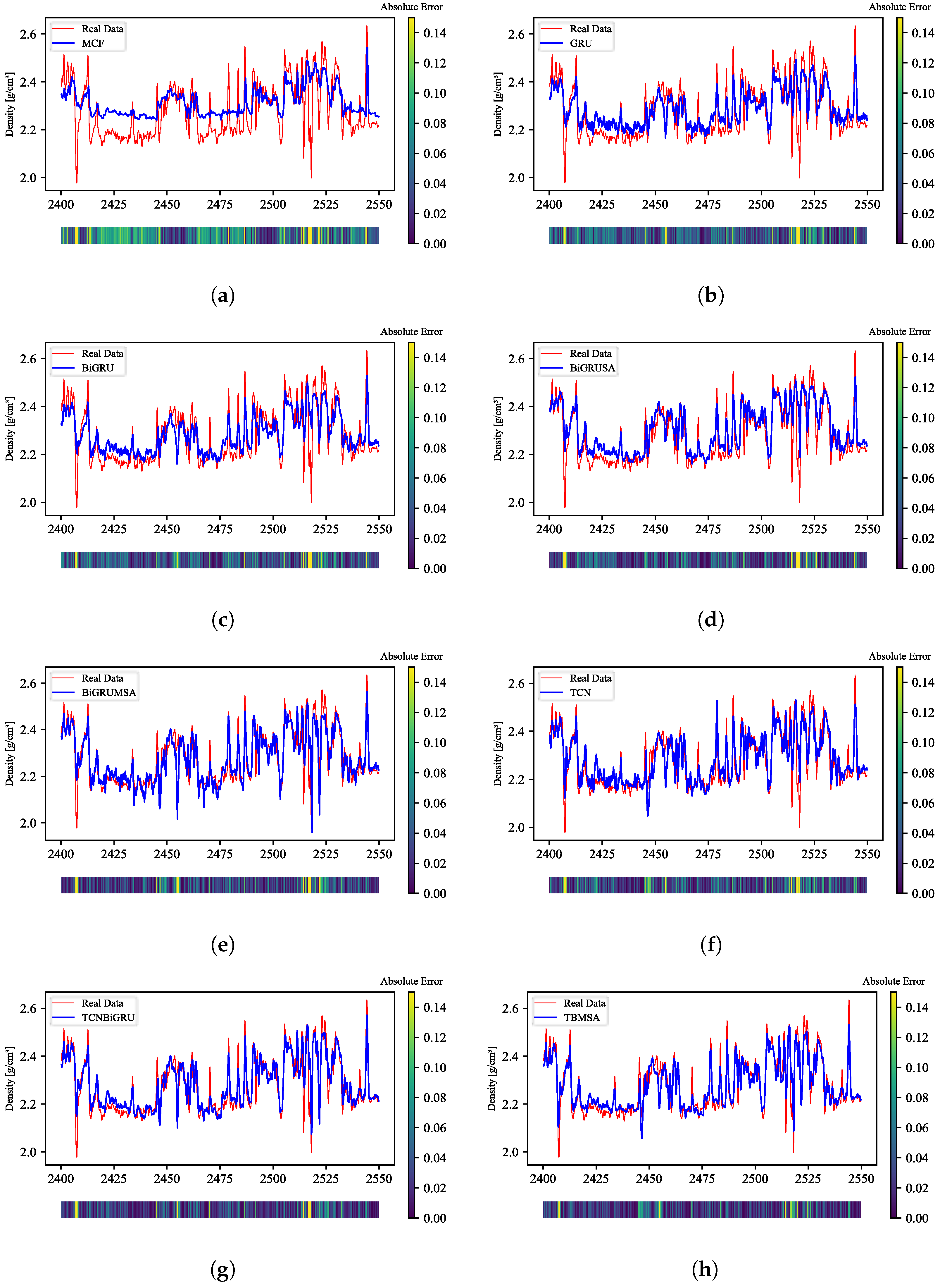
3.3.2. Experimental Results Analysis

Figure 9 and Table 3 detail the outcomes and discrepancies related to the DEN curve’s reconstruction. Additionally, the comparative impacts on curve restoration from eight diverse techniques, identified from (a) to (h), are depicted in Figure 9, using color blocks to represent the absolute errors between curves. The figure clearly demonstrates that the reconstruction techniques depicted in images (e) to (h) yield superior results relative to those shown in images (a) to (d). For a more comprehensive assessment of the curve reconstruction’s efficacy, evaluation metrics such as mean absolute error (MAE), mean squared error (MSE), and root mean squared error (RMSE) were employed. Analysis of the data in Table 3 indicates that the TBMSA model performs the best. Methods which employ deep learning techniques outperform those which use multivariate fitting for reconstruction. Models which incorporate the TCN module demonstrate superior performance over those that do not; BiGRU shows better reconstruction effects compared to GRU, and model performance is further enhanced after the MSA module is integrated.

Figure 9. Comparison of density curve reconstruction results using eight different methods. (a–h) represent the reconstruction using each of the eight methods, respectively. The red curve signifies the true density values, whereas the blue curve denotes the estimated density values. The shaded regions illustrate the magnitude of absolute error between the actual and predicted values. By comparing the color scale and curves, it can be observed that the reconstruction effect in panel (h) is superior.

Table 3. Reconstruction errors of various models.

Evaluation Indicators	MAE	MSE	RMSE
MCF	0.0695	0.0074	0.0863
GRU	0.0491	0.0039	0.0625
BiGRU	0.0454	0.0036	0.0599
BiGRU-SA	0.0403	0.0033	0.0578
BiGRU-MSA	0.0385	0.0030	0.0547
TCN	0.0399	0.0029	0.0542
TCN-BiGRU	0.0332	0.0023	0.0481
TBMSA	0.0303	0.0018	0.0421

3.4. Core Calibration Experiment

To assess the generalization ability of the CTBMSA model, the completely trained model was utilized to reconstruct the density curves in two unseen wells, C and D, situated within the identical stratigraphic layer. Core density measurements from wells C and D were selected for core calibration experiments on the reconstructed curves, with results shown in Figure 10a,b. In the third track of these two figures, Core-DEN represents core density, DEN-CTBMSA repersents reconstructed density, and DEN for compensated density. In Figure 10a, the depth interval from 4100 m to 4113 m represents a slight borehole enlargement section; in Figure 10b, the depth interval from 369 0m to 3707 m represents a severe borehole enlargement section, and the interval from 3712 m to 3720 m represents a non-enlarged section. It can be clearly observed in the figures that compared to actual measured curves, the density curves reconstructed by the CTBMSA model under three different geological conditions show a high consistency with the core densities. Furthermore, despite the varying degrees of borehole enlargement and the constraints of the borehole diameter curves and stratigraphic lithology indicators, the model can reconstruct the density curves with high accuracy, even in the presence of severe enlargement. This indicates that through extensive data training, the model has learned the intrinsic correlations of the curves and possesses a high generalization capability.

Figure 10. (a) illustrates the calibration of reconstructed curves with core data for Well C, and (b) shows the calibration for Well D. “CAL” denotes the borehole diameter curve, and “Core-DEN” represents core density data. The blue curve indicates the density curve obtained from actual measurements, while the red curve represents the model-predicted curve.

4. Conclusions

This study thoroughly explores the application and critical importance of well logging curve reconstruction in oil and gas exploration and development. Given the complex and variable nature of geological formations and the limitations of measurement technologies, the distortion or absence of well logging curves is a common issue, posing significant challenges for subsequent geological interpretation and evaluation. While traditional reconstruction methods, such as empirical formulae, multiple regression methods, and rock physics modeling, are effective under specific conditions, they often perform poorly when dealing with complex geological structures. This study emphasizes the value of deep learning techniques, particularly a model that integrates TCN, Bi-GRU, and self-attention mechanisms, supplemented with physical constraints, in improving the accuracy and efficiency of well logging curve reconstruction.

Density curve reconstruction experiments were conducted on four wells in an exploration and development area of the X depression. Initially, comparative analysis on Well A validated the role of physical constraints in enhancing model fitting capability. Subsequently, the proposed method was compared with seven other methods, and the experimental results demonstrated that the proposed TBMSA method achieved high accuracy in reconstructing density curves. Finally, core calibration experiments on Wells C and D proved that the model possesses a strong generalization capability, making it valuable for practical production applications and particularly effective in addressing density curve distortions caused by borehole enlargement.

Although the proposed method can reconstruct curves with high accuracy, and despite its feasibility being validated through core comparison experiments in actual work areas, this study primarily focuses on sandstone and shale formations. Therefore, further research and validation are required for its applicability to more complex carbonate and igneous rock regions.

References

- Zhang, D.; Chen, Y.; Meng, J. Synthetic well logs generation via Recurrent Neural Networks. Pet. Explor. Dev. 2018, 45, 629–639. [Google Scholar] [CrossRef]
- Fan, P.; Deng, R.; Qiu, J.; Zhao, Z.; Wu, S. Well logging curve reconstruction based on kernel ridge regression. Arab. J. Geosci. 2021, 14, 1–10. [Google Scholar] [CrossRef]
- Lin, L.; Wei, H.; Wu, T.; Zhang, P.; Zhong, Z.; Li, C. Missing well-log reconstruction using a sequence self-attention deep-learning framework. Geophysics 2023, 88, D391–D410. [Google Scholar] [CrossRef]
- Zhang, H.; Wu, W.; Song, X. Well Logs Reconstruction Based on Deep Learning Technology. IEEE Geosci. Remote Sens. Lett. 2024. [CrossRef]
- Ming, L.; Deng, R.; Gao, C.; Zhang, R.; He, X.; Chen, J.; Zhou, T.; Sun, Z. Logging curve reconstructions based on MLP multilayer perceptive neural network. Int. J. Oil Gas Coal Technol. 2023, 34, 25–41. [Google Scholar] [CrossRef]
- Ren, Q.; Zhang, H.; Azevedo, L.; Yu, X.; Zhang, D.; Zhao, X.; Zhu, X.; Hu, X. Reconstruction of Missing Well-Logs Using Facies-Informed Discrete Wavelet Transform and Time Series Regression. SPE J. 2023, 28, 2946–2963. [Google Scholar] [CrossRef]
- Zhang, G.; Wang, Z.; Chen, Y. Deep learning for seismic lithology prediction. Geophys. J. Int. 2018, 215, 1368–1387. [Google Scholar] [CrossRef]
- You, L.; Tan, Q.; Kang, Y.; Xu, C.; Lin, C. Reconstruction and prediction of capillary pressure curve based on Particle Swarm Optimization-Back Propagation Neural Network method. Petroleum 2018, 4, 268–280. [Google Scholar] [CrossRef]
- Mo, X.; Zhang, Q.; Li, X. Well logging curve reconstruction based on genetic neural networks. In Proceedings of the 2015 12th International Conference on Fuzzy Systems and Knowledge Discovery (FSKD), Zhangjiajie, China, 15–17 August 2015; pp. 1015–1021. [Google Scholar]
- Jun, W.; Jun-xing, C.; Jia-chun, Y. Log reconstruction based on gated recurrent unit recurrent neural network. In Proceedings of the SEG 2019 Workshop: Mathematical Geophysics: Traditional vs Learning, Beijing, China, 5–7 November 2019; pp. 91–94. [Google Scholar]
- Zeng, L.; Ren, W.; Shan, L.; Huo, F. Well logging prediction and uncertainty analysis based on recurrent neural network with attention mechanism and Bayesian theory. J. Pet. Sci. Eng. 2022, 208, 109458. [Google Scholar] [CrossRef]
- Cheng, C.; Gao, Y.; Chen, Y.; Jiao, S.; Jiang, Y.; Yi, J.; Zhang, L. Reconstruction Method of Old Well Logging Curves Based on BI-LSTM Model—Taking Feixianguan Formation in East Sichuan as an Example. Coatings 2022, 12, 113. [Google Scholar] [CrossRef]
- Chang, J.; Li, J.; Liu, H.; Kang, Y.; Lv, W. Well Logging Reconstruction Based on Bidirectional GRU. In Proceedings of the 2022 2nd International Conference on Control and Intelligent Robotics, Nanjing China, 24–26 June 2022; pp. 525–528. [Google Scholar]
- Li, J.; Gao, G. Digital construction of geophysical well logging curves using the LSTM deep-learning network. Front. Earth Sci. 2023, 10, 1041807. [Google Scholar] [CrossRef]
- Zhang, H.; Wu, W.; Chen, Z.; Jing, J. Well logs reconstruction of petroleum energy exploration based on bidirectional Long Short-term memory networks with a PSO optimization algorithm. Geoenergy Sci. Eng. 2024, 239, 212975. [Google Scholar] [CrossRef]
- Zhou, X.; Zhang, Z.; Zhang, C. Bi-LSTM deep neural network reservoir classification model based on the innovative input of logging curve response sequences. IEEE Access 2021, 99. [Google Scholar]
- Li, G.; Chen, W.; Mu, C. Residual-wider convolutional neural network for image recognition. IET Image Process. 2020, 14, 4385–4391. [Google Scholar] [CrossRef]
- Zhang, J.; Shao, K.; Luo, X. Small sample image recognition using improved Convolutional Neural Network. J. Vis. Commun. Image Represent. 2018, 55, 640–647. [Google Scholar] [CrossRef]
- Gu, J.; Wang, Z.; Kuen, J.; Ma, L.; Shahroudy, A.; Shuai, B.; Liu, T.; Wang, X.; Wang, G.; Cai, J.; et al. Recent advances in convolutional neural networks. Pattern Recognit. 2018, 77, 354–377. [Google Scholar] [CrossRef]
- Shamsipour, G.; Fekri-Ershad, S.; Sharifi, M.; Alaei, A. Improve the efficiency of handcrafted features in image retrieval by adding selected feature generating layers of deep convolutional neural networks. Signal Image Video Process. 2024, 18, 2607–2620. [Google Scholar] [CrossRef]
- Wu, L.; Dong, Z.; Li, W.; Jing, C.; Qu, B. Well-logging prediction based on hybrid neural network model. Energies 2021, 14, 8583. [Google Scholar] [CrossRef]
- Duan, Z.Y.; Wu, Y.; Xiao, Y.; Li, C.L. Density logging curve reconstruction method based on CGAN and CNN-GRU combined model. Prog. Geophys. 2022, 37, 1941–1945. [Google Scholar]
- Wang, J.; Cao, J.; Fu, J.; Xu, H. Missing well logs prediction using deep learning integrated neural network with the self-attention mechanism. Energy 2022, 261, 125270. [Google Scholar] [CrossRef]
- Bai, S.; Kolter, J.Z.; Koltun, V. An empirical evaluation of generic convolutional and recurrent networks for sequence modeling. arXiv 2018, arXiv:1803.01271. [Google Scholar]
- Jiang, C.; Zhang, D.; Chen, S. Lithology identification from well-log curves via neural networks with additional geologic constraint. Geophysics 2021, 86, IM85–IM100. [Google Scholar] [CrossRef]
- Cai, C.; Li, Y.; Su, Z.; Zhu, T.; He, Y. Short-term electrical load forecasting based on VMD and GRU-TCN hybrid network. Appl. Sci. 2022, 12, 6647. [Google Scholar] [CrossRef]
- Wang, D.; Chen, G. Intelligent seismic stratigraphic modeling using temporal convolutional network. Comput. Geosci. 2023, 171, 105294. [Google Scholar] [CrossRef]
- He, K.; Zhang, X.; Ren, S.; Sun, J. Deep residual learning for image recognition. In Proceedings of the IEEE Conference on Computer Vision and Pattern Recognition, Las Vegas, NV, USA, 26 June–1 July 2016; pp. 770–778. [Google Scholar]
- Yu, Z.; Sun, Y.; Zhang, J.; Zhang, Y.; Liu, Z. Gated recurrent unit neural network (GRU) based on quantile regression (QR) predicts reservoir parameters through well logging data. Front. Earth Sci. 2023, 11, 1087385. [Google Scholar] [CrossRef]
- Chung, J.; Gulcehre, C.; Cho, K.H.; Bengio, Y. Empirical evaluation of gated recurrent neural networks on sequence modeling. arXiv 2014, arXiv:1412.3555. [Google Scholar]
- She, D.; Jia, M. A BiGRU method for remaining useful life prediction of machinery. Measurement 2021, 167, 108277. [Google Scholar] [CrossRef]
- Qiao, Y.; Xu, H.M.; Zhou, W.J.; Peng, B.; Hu, B.; Guo, X. A BiGRU joint optimized attention network for recognition of drilling conditions. Pet. Sci. 2023, 20, 3624–3637. [Google Scholar] [CrossRef]
- Bahdanau, D.; Cho, K.; Bengio, Y. Neural machine translation by jointly learning to align and translate. arXiv 2014, arXiv:1409.0473. [Google Scholar]
- Zeng, L.; Ren, W.; Shan, L. Attention-based bidirectional gated recurrent unit neural networks for well logs prediction and lithology identification. Neurocomputing 2020, 414, 153–171. [Google Scholar] [CrossRef]
- Yang, L.; Wang, S.; Chen, X.; Chen, W.; Saad, O.M.; Zhou, X.; Pham, N.; Geng, Z.; Fomel, S.; Chen, Y. High-fidelity permeability and porosity prediction using deep learning with the self-attention mechanism. IEEE Trans. Neural Netw. Learn. Syst. 2022, 34, 3429–3443. [Google Scholar] [CrossRef] [PubMed]
- Liu, N.; Li, Z.; Liu, R.; Zhang, H.; Gao, J.; Wei, T.; Wu, H. ASHFormer: Axial and sliding window based attention with high-resolution transformer for automatic stratigraphic correlation. IEEE Trans. Geosci. Remote Sens. 2023, 61, 5913910. [Google Scholar] [CrossRef]
Disclaimer/Publisher’s Note: The statements, opinions and data contained in all publications are solely those of the individual author(s) and contributor(s) and not of MDPI and/or the editor(s). MDPI and/or the editor(s) disclaim responsibility for any injury to people or property resulting from any ideas, methods, instructions or products referred to in the content. |
© 2024 by the authors. Licensee MDPI, Basel, Switzerland. This article is an open access article distributed under the terms and conditions of the Creative Commons Attribution (CC BY) license (https://creativecommons.org/licenses/by/4.0/).