Optimal Scheduling of Zero-Carbon Parks Considering Flexible Response of Source–Load Bilaterals in Multiple Timescales

Abstract

In order to enhance the carbon reduction potential of a park, a low-carbon economic dispatch method applicable to zero-carbon parks is proposed to optimize the energy dispatch of the park at multiple timescales; this is achieved by introducing a flexible response mechanism for source–load bilaterals, so as to achieve low-carbon, economic, and efficient operation. First, a park model that accounts for the energy flow characteristics and carbon potential distribution of the energy hub is established. Then, based on the flexible operation of energy supply equipment and multi-type integrated demand response, the flexible response mechanism of source–load bilaterally and the multi-timescale scheduling framework are proposed; the mechanisms of source–load coordination and electricity–carbon coupling are analyzed in depth. Finally, with the objective of optimal system operation economy, the optimal scheduling model is established for three timescales, namely, day-ahead, intraday, and real-time scheduling. The equipment output and demand response are optimized step by step according to the source–load prediction information and scheduling results at each stage. The simulation results show that the proposed model can effectively utilize the source and load resources to participate in scheduling and can effectively reduce carbon emissions while ensuring the energy supply demand of the park, realizing the low-carbon, economic operation of the system. Therefore, this study provides a new theoretical basis and practical solution for the optimal dispatch of energy in zero-carbon parks, which helps to promote the development of a low-carbon economy.

1. Introduction

With peak carbon and carbon neutral targets, the unstable, uneconomic, and unclean contradiction of energy utilization between the energy supply side and the demand side has become particularly prominent [1,2]. With the aggravation of environmental pollution and energy scarcity, it is crucial to establish a modern energy system that is clean, low-carbon, safe, and efficient [3]. As one of the main energy users, the zero-carbon park covers a variety of energy forms such as electricity, cooling energy, and heat energy [4]. A zero-carbon park is not completely free of greenhouse gas emissions, but rather has zero net carbon emissions over a certain period of time. A carbon-neutral park is a systematic project which can be considered from the aspects of energy, buildings, transportation, carbon sinks, and management, and includes multiple types of energy storage, carbon capture, multi-energy synergy, demand response, and other technologies [5,6]. In order to encourage the development of low-carbon electricity and increase the capacity of renewable energy consumption, it is crucial to research how zero-carbon parks operate [7].

Demand-side resources are crucial in encouraging the park to operate with a low carbon footprint. The authors of [8] suggest a fuzzy logic-based integrated demand response approach that takes changing heat price into account and modifies indoor temperature setpoints accordingly. The authors of [9] proposed a carbon capture plant optimization method considering a low-carbon demand response, which guides the load side to take responsibility for the carbon emissions. The authors of [10] proposed a demand response elasticity subsidy strategy counting the degree of time-vacancy loading, which improves the system regulation operation’s economy and cleanliness. The authors of [11] provided an integrated zero-carbon plant operation optimization model that takes into account the green value and encourages the potential for new energy consumption, combining unpredictable green energy, adjustable loads, and energy storage resources into a whole in a grid-friendly manner. The authors of [12] proposed a large-scale demand response implementation method based on direct customer loads to improve system stability in response to the problem of increased peak pressure on thermal power units due to a high proportion of new energy sources being connected to the grid. The authors of [13] proposed a methodology for evaluating customer demand response measures and metrics to provide energy flexibility during periods of grid stress.

The sources from the literature mentioned above only look at the flexible regulation of load-side demand response in system operation to improve the economy; however, the impact of single load-side demand response on the energy system is limited, and the above literature does not consider the energy-side response and uncertainty issues [14]. To improve this problem, ref. [15] effectively solved the system wind abandonment and supply–demand imbalance problems by coordinating the demand response resources with thermal storage electric heating and multi-timescale characteristics while improving the system’s flexible regulation capability; ref. [16] developed a stochastic day-ahead scheduling model for grid-connected wind power that effectively lowers overall carbon emissions by including a carbon capture power plant and coupon-based demand response; based on consumer psychology, ref. [17] established an integrated demand response model that takes uncertainty into account, and when demand response behavioral interventions alter the energy system configuration and transaction prices, a Nash-type game is employed to guarantee the transaction’s fairness. This enhances the economics of both the demand response aggregator and the energy retailer.

In general, the above literature has made significant progress in the study of low-carbon economic optimization of park operations, but there are still the following shortcomings: ① in the process of achieving carbon neutrality, the issue of how to accurately assess and monitor the park’s carbon emissions remains a technical and methodological challenge, and the integration and optimization of the various resources within the park remains complex [18,19]; ② existing studies on carbon-neutral technologies only consider the energy supply side or the load side, failing to realize the coordination between sources and loads, and failing to provide dynamic feedback on changes in energy use and adjust the balance between supply and demand in real time [20,21]; ③ most of the existing studies have only considered the “heat for power” or “power for heat” operations of combined heat and power (CHP) equipment during the day-ahead scheduling phase, which is limited and cannot meet the demand for flexible system operation [22,23]; ④ in multi-timescale optimal scheduling, the studies of existing models do not go deep enough into the actual responsiveness of energy equipment and the response characteristics of demand-side resources, failing to effectively integrate and optimize source–load flexibility resources [24]. Therefore, in order to satisfy the optimal scheduling of zero-carbon parks under multiple timescales, it is necessary to deeply excavate the response characteristics of demand-side resources and establish a flexible response model of multi-timescale source–load bilaterals under the consideration of source–load coordination and electricity–carbon coupling, so as to enable the parks to realize zero-carbon operations [25].

To address the aforementioned issues, this paper develops a flexible operation equipment model on the energy supply side, a demand response model on the demand side that takes into account various response characteristics, and a flexible response model on both the source and load sides. Second, the source–load bilateral flexible response mechanism is analyzed and a multi-timescale scheduling framework is proposed. Finally, the ideal scheduling model for the zero-carbon park is constructed, taking into account the flexible response of both sources and loads across numerous timescales, and the park’s actual operating outcomes across various timescales are investigated. The usefulness of the model suggested in this research for enhancing system economy and low-carbon performance is confirmed by comparing it to various simulated situations.

2. Zero-Carbon Park Structure Based on Energy Hubs

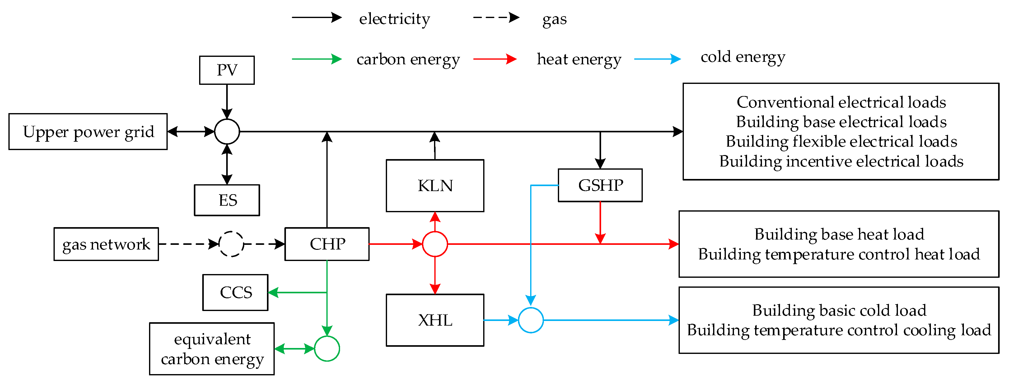
2.1. Structure of the Park

A zero-carbon park refers to the application of renewable energy, carbon capture and storage technology, and energy storage and management within a certain area, with a view to minimizing carbon emissions or even achieving carbon neutrality in energy, industry, buildings, and other areas within the park. Zero-carbon parks do not only rely on reducing energy consumption, but also include compensating for or eliminating the remaining carbon emissions through various means, in order to achieve the goal of “zero emissions” across the board [26,27].

The research framework of this paper is shown in Figure 1, and the energy supply side includes the superior grid, natural gas grid, and photovoltaic units (PVs); the energy conversion equipment includes CHP, Kalina cycle power generation equipment (KLN), lithium bromide absorption refrigeration equipment (XHL), ground-source heat pumps (GSHP), carbon capture and storage equipment (CCS), and equivalent carbon streams (including natural carbon sinks and carbon trading); the energy storage equipment includes electric energy storage (ES); the load side includes electric loads, heat loads, and cold loads. The details of the types of loads are shown in Figure 1.

2.2. Characterization of Energy Flows in Energy Hubs

The load side of the park can optimize its own energy demand through energy coupling equipment according to the different energy prices provided by the supply side on the one hand [28]; on the other hand, it can fill in the shortfall by adjusting complementary energy equipment when part of the resources are in short supply and cannot be fulfilled, e.g., electricity demand can be fulfilled by the grid, PV, and CHP; heat demand can be fulfilled by CHP and GSHP; cooling demand can be fulfilled by XHL and GSHP. The energy coupling relationship is shown in Equation (1).

$$\left[\begin{array}{l}{D}_{\mathrm{e}}\\ D_{\mathrm{h}}\\ D_{\mathrm{c}}\end{array}\right]=\left[\begin{array}{ccc}{\alpha }_{\mathrm{e}}& {\eta }_{\mathrm{e}}^{\mathrm{CHP}}& {\beta }_{\mathrm{KLN}}{\eta }_{\mathrm{e}}^{\mathrm{KLN}}\\ {\alpha }_{\mathrm{GSHP}}{\eta }_{\mathrm{h}}^{\mathrm{GSHP}}& 0& {\beta }_{\mathrm{h}}\\ {\alpha }_{\mathrm{GSHP}}{\eta }_{\mathrm{c}}^{\mathrm{GSHP}}& 0& {\beta }_{\mathrm{XHL}}{\eta }_{\mathrm{c}}^{\mathrm{XHL}}\end{array}\right]\left[\begin{array}{l}{E}_{\mathrm{e}}\\ E_{\mathrm{g}}\\ E_{\mathrm{h}}\end{array}\right]$$

(1)

where $D_{\mathrm{e}}$, $D_{\mathrm{h}}$, and $D_{\mathrm{c}}$ denote the demand for electricity, heat, and cold, respectively; $E_{\mathrm{e}}$, $E_{\mathrm{g}}$, and $E_{\mathrm{h}}$ denote the power, gas, and heat sources, respectively; ${\alpha }_{\mathrm{e}}$ and ${\alpha }_{\mathrm{GSHP}}$ denote the demand for electricity and the distribution coefficients of GSHP in the power source, respectively; ${\beta }_{\mathrm{h}}$, ${\beta }_{\mathrm{KLN}}$, and ${\beta }_{\mathrm{XHL}}$ denote the demand for heat and the distribution coefficients of the KLN and XHL in the heat source, respectively; ${\eta }_{\mathrm{h}}^{\mathrm{GSHP}}$ and ${\eta }_{\mathrm{c}}^{\mathrm{GSHP}}$ denote the efficiency of GSHP in heat production and cooling, respectively; ${\eta }_{\mathrm{e}}^{\mathrm{CHP}}$ denotes the efficiency of CHP in power generation; ${\eta }_{\mathrm{e}}^{\mathrm{KLN}}$ denotes the efficiency of KLN in power generation; ${\eta }_{\mathrm{c}}^{\mathrm{XHL}}$ represents the cooling efficiency of XHL. Among them, the distribution coefficient is related to the type and distribution of loads and can be flexibly adjusted according to the load side.

2.3. Energy Hub Modeling Considering Carbon Potential Distribution

To learn how to lower carbon emissions, it is necessary to analyze the sources of the emissions produced when the park is in operation. Carbon emissions may be efficiently decreased, and the energy system’s operation can be more precisely controlled by examining the distribution and change patterns of the pooled carbon potential on the energy hub (EH) [29,30].

Let the park have $N$ EHs, $K$ energy supply equipment, and $M$ loads; then, the injected power of EHs is shown in Equation (2).

$$P_i^{\mathrm{EH}}={\displaystyle \sum _{d\in I^{+}}^D{P}_d^{\mathrm{B}}}+{\displaystyle \sum _{k\in I^{+}}^K{P}_k^{\mathrm{G}}}$$

(2)

where $P_i^{\mathrm{EH}}$ denotes the total active power injected by the $i$ EH; $P_d^{\mathrm{B}}$ denotes the power injected by the $d$ upstream branch; $P_k^{\mathrm{G}}$ denotes the power accessed by the $k$ energy supply equipment; $I^{+}$ denotes the set of all upstream branches accessed by the EH; $D$ denotes the set of upstream branches except for the energy supply equipment; and $D$ and $K$ satisfy the requirement of $D+K=I^{+}$.

The EH pooling carbon potential $e_i^{\mathrm{EH}}$ is determined by a combination of the carbon intensity of the connected energy supply equipment and the carbon flow density of the remaining upstream branches, as shown in Equation (3).

$$e_i^{\mathrm{EH}}={\displaystyle \frac{{{\displaystyle \sum }}_{d\in I^{+}}^D{P}_d^{\mathrm{B}}{\rho }_d^{\mathrm{B}}+{{\displaystyle \sum }}_{k\in I^{+}}^K{P}_k^{\mathrm{G}}{e}_k^{\mathrm{G}}}{{{\displaystyle \sum }}_{d\in I^{+}}^D{P}_d^{\mathrm{B}}+{{\displaystyle \sum }}_{k\in I^{+}}^K{P}_k^{\mathrm{G}}}}$$

(3)

where ${\rho }_d^{\mathrm{B}}$ denotes the carbon flow intensity of the feeder road $d$; $e_k^{\mathrm{G}}$ denotes the carbon emission intensity of the energy supply equipment $k$.

The traditional and renewable energy sources connected to the EH in the park are regarded as energy inputs; the energy storage is regarded as an input when discharging and an output when charging. The energy coupling matrix $C$ is constructed based on the power distribution between various energy sources and different loads in the system, as shown in Equation (4).

$$P^{\mathrm{L}}=C\times {\left[P^{\mathrm{B}}{P}^{\mathrm{G}}\right]}^{\mathrm{T}}$$

(4)

where $P^{\mathrm{L}}={\left[P_{m,i}^{\mathrm{L}}\right]}_{M\times N}$ denotes an $M\times \mathrm{N}$-order load distribution matrix; $P^{\mathrm{B}}={\left[P_{d,i}^{\mathrm{B}}\right]}_{D\times N}$ denotes a $D\times N$-order branch distribution matrix; $P^{\mathrm{G}}={\left[P_{k,i}^{\mathrm{G}}\right]}_{K\times N}$ denotes a $K\times N$-order energy supply equipment branch distribution matrix; $C={\left[C_{m,k^{\ast }}\right]}_{M\times (D+K)}$ denotes an $M\times \left(D+K\right)$-order energy coupling matrix.

The total carbon emissions flowing through the EH during the dispatch cycle $T$$Q_l^{\mathrm{EH}}$ are shown in Equation (5).

$$Q_l^{\mathrm{EH}}={\displaystyle \sum }_{i=1}^N{\displaystyle \sum }_{t=1}^T{P}_{m,i}^{\mathrm{L}}{\rho }_{m,i}^{\mathrm{L}}\Delta t$$

(5)

where $P_{m,i}^{\mathrm{L}}$ and ${\rho }_{m,i}^{\mathrm{L}}$ denote the active power and carbon flow density flowing into the load from EH, respectively; $\Delta t$ denotes the scheduling step.

3. Source–Load Bilateral Flexible Response Model and Operation Mechanism

The energy types in the park are differentiated and complementary, and the shortages are filled by adjusting complementary energy equipment. There have been more studies on the modeling of Section 2.1 equipment at home and abroad [31,32]; the details of the conventional equipment model will not be discussed, and only the more innovative or application-specific modeling methods will be analyzed.

3.1. Equipment Model

3.1.1. Modeling of Equipment Operation in Variable Conditions

CHP unit is a natural-gas-fueled device capable of generating electrical and thermal energy; considering its variable operating condition characteristics, the CHP electric–thermal coupling characteristic model is shown in Equation (6).

$$\left\{\begin{array}{l}{P}_{\mathrm{e},t}^{\mathrm{CHP}}\ge U_t^{\mathrm{CHP}}{P}_{\mathrm{e},\min }^{\mathrm{CHP}}\\ P_{\mathrm{e},t}^{\mathrm{CHP}}\ge U_t^{\mathrm{CHP}}[P_{\mathrm{e},0}^{\mathrm{CHP}}+k_2(P_{\mathrm{h},t}^{\mathrm{CHP}}-P_{\mathrm{h},\max }^{\mathrm{CHP}})]\\ P_{\mathrm{e},t}^{\mathrm{CHP}}\le U_t^{\mathrm{CHP}}[P_{\mathrm{e},\max }^{\mathrm{CHP}}+k_1(P_{\mathrm{h},\max }^{\mathrm{CHP}}-P_{\mathrm{h},t}^{\mathrm{CHP}})]\\ P_{\mathrm{h},t}^{\mathrm{CHP}}\ge 0\\ U_t^{\mathrm{CHP}}\in \{0,1\}\end{array}\right.$$

(6)

where $P_{\mathrm{e},t}^{\mathrm{CHP}}$ and $P_{\mathrm{h},t}^{\mathrm{CHP}}$ denote the generation power and heat generation power of CHP;$P_{\mathrm{e},\max }^{\mathrm{CHP}}$ and $P_{\mathrm{e},\min }^{\mathrm{CHP}}$ denote the upper and lower limits of generation power of CHP; $P_{\mathrm{h},\max }^{\mathrm{CHP}}$ denotes the maximum heat generation power of CHP; $P_{\mathrm{e},0}^{\mathrm{CHP}}$ denotes the generation power corresponding to the maximum heat generation power of CHP; $k_1$ and $k_2$ denote the upper limit and lower limit slopes of CHP’s electric-heat coupling interval; and $U_t^{\mathrm{CHP}}$ denotes the start–stop state identification bit of CHP.

3.1.2. Flexible Operation Model for Carbon Capture Devices

CCS can alleviate the conflict between load demand and carbon capture energy consumption and improve the energy utilization efficiency by selectively emitting CO₂ during the peak electricity consumption period and shifting the energy consumption to the low valley period [33], and the operation model is shown in Equation (7).

$$\left\{\begin{array}{l}{P}_{\mathrm{e},t}^{\mathrm{CCS}}=P_{\mathrm{c},t}^{\mathrm{CCS}}+P_{\mathrm{r},t}^{\mathrm{CCS}}\\ P_{\mathrm{r},t}^{\mathrm{CCS}}={\eta }^{\mathrm{ccs}}{Q}_t^{\mathrm{CCS}}\\ Q_{\mathrm{G},t}^{\mathrm{CCS}}={\mathrm{e}}_{\mathrm{G}}{P}_{\mathrm{e},t}^{\mathrm{G}}\\ Q_{\mathrm{cur},t}^{\mathrm{CCS}}=\left(1-{\eta }^{\mathrm{CCS}}\right)Q_{\mathrm{G},t}^{\mathrm{CCS}}\\ {\eta }_{\min }^{\mathrm{CCS}}\le {\eta }^{\mathrm{CCS}}\le {\eta }_{\max }^{\mathrm{CCS}}\end{array}\right.$$

(7)

where $P_{\mathrm{e},t}^{\mathrm{CCS}}$ represents the total power consumption of CCS at $t$; $P_{\mathrm{c},t}^{\mathrm{CCS}}$ and $P_{\mathrm{r},t}^{\mathrm{CCS}}$ represent the fixed energy consumption and operational energy consumption of CCS at $t$; ${\eta }^{\mathrm{ccs}}$ represents the energy consumption coefficient of capturing a unit of CO₂; $Q_t^{\mathrm{CCS}}$ and $Q_{\mathrm{G},t}^{\mathrm{CCS}}$ represent the actual amount of CO₂ captured by CCS and the total amount of CO₂ generated by thermal power units; $P_{\mathrm{e},t}^{\mathrm{G}}$ represents the total power of generating units at $t$; ${\mathrm{e}}_{\mathrm{G}}$ represents the carbon emission coefficient of the generating units; $Q_{\mathrm{cur},t}^{\mathrm{CCS}}$ represents the total amount of CO₂ that has escaped into the atmosphere after the capture; ${\eta }^{\mathrm{CCS}}$ represents the capture efficiency of CCS; ${\eta }_{\max }^{\mathrm{CCS}}$ and ${\eta }_{\min }^{\mathrm{CCS}}$ denote the upper and lower limits of carbon capture efficiency, respectively.

3.2. Load Response Modeling

In order to fully exploit the responsiveness of demand-side resources, they are classified into three types of responsive loads, including price-based demand response (PDR), which takes into account the carbon potential correction, incentive-based demand response (IDR) considering different response rates, and temperature-based demand response (TDR) considering heat conduction in the building.

3.2.1. PDR Model Considering Carbon Potential Correction

The expression for the tariff elasticity factor of the load is shown in Equation (8).

$${\displaystyle \frac{\Delta Q_i}{Q_i}}={\epsilon }_{ij}{\displaystyle \frac{\Delta P_j}{P_j}}$$

(8)

where $Q_i$ and $\Delta Q_i$ denote the initial load power and load response power at the time of $i$; $P_i$ and $\Delta P_i$ denote the initial tariff and price change at the time of $j$; when $i=j$, ${\epsilon }_{ij}$ denotes the self-elasticity coefficient; when $i\ne j$, ${\epsilon }_{ij}$ denotes the cross-elasticity coefficient.

In order to regulate the load-side demand response in a more refined way and reflect the impact of electricity price change on carbon potential change, this paper divides the electricity price change quantity $\Delta P_j$ into time-sharing electricity price change quantity $\Delta P_j^{\mathrm{S}}$ (primary adjustment) and carbon potential correction electricity price change quantity $\Delta P_j^{\mathrm{R}}$ (secondary adjustment), and introduces the carbon potential correction coefficient ${\sigma }_{ij}$ to regulate the impact of the electricity price change on the structure of the energy composition, as shown in Equations (9) and (10).

$$\Delta P_j=\Delta P_j^{\mathrm{S}}+\Delta P_j^{\mathrm{R}}$$

(9)

$${\displaystyle \frac{\Delta P_j^{\mathrm{R}}}{\Delta P_j}}={\sigma }_{ij}{\displaystyle \frac{\Delta e_i}{e_i}}$$

(10)

where when $i=j$, ${\sigma }_{ij}$ denotes the self-correction factor; when $i\ne j$, ${\sigma }_{ij}$ denotes the cross-correction factor.

The correction factor and elasticity factor of the load can be divided according to the time period, as shown in Equations (11) and (12).

$$\mathit{\Gamma }=\left[\begin{array}{ccc}{\sigma }^{\mathrm{ff}}& {\sigma }^{\mathrm{fp}}& {\sigma }^{\mathrm{fg}}\\ {\sigma }^{\mathrm{pf}}& {\sigma }^{\mathrm{pp}}& {\sigma }^{\mathrm{pg}}\\ {\sigma }^{\mathrm{gf}}& {\sigma }^{\mathrm{gp}}& {\sigma }^{\mathrm{gg}}\end{array}\right]$$

(11)

$$\mathit{E}=\left[\begin{array}{ccc}{\epsilon }^{\mathrm{ff}}& {\epsilon }^{\mathrm{fp}}& {\epsilon }^{\mathrm{fg}}\\ {\epsilon }^{\mathrm{pf}}& {\epsilon }^{\mathrm{pp}}& {\epsilon }^{\mathrm{pg}}\\ {\epsilon }^{\mathrm{gf}}& {\epsilon }^{\mathrm{gp}}& {\epsilon }^{\mathrm{gg}}\end{array}\right]$$

(12)

where $\mathrm{f}$, $\mathrm{p}$, and $\mathrm{g}$ correspond to the peak, level, and trough periods, respectively.

The combined Equations (8)–(12) can be derived as the demand of the load in each time period after the PDR response $Q^{\mathrm{op}}$, as shown in Equation (13).

$${\mathit{Q}}^{\mathrm{op}}=\mathit{Q}+\mathrm{diag}(\mathit{Q})\mathit{E}\Delta {\mathit{P}}^{\mathit{S}}{\mathit{P}}^{-1}(\mathit{\eta }-\mathit{\Gamma }\Delta {\mathit{ee}}^{-1})$$

(13)

3.2.2. IDR Model Considering Different Response Rates

Incentive-based demand response loads are sold by the customer to the park with controllable capacity according to the forecasted power plan, and the total power before and after IDR loads satisfy the demand response remains unchanged, as shown in Equation (14).

$${\displaystyle \sum _{t_f}^{t_b}{P}_{\mathrm{e},i,t}^{\mathrm{IDR}}}={\displaystyle \sum _{t_f}^{t_b}{\tilde{P}}_{\mathrm{e},i,t}^{\mathrm{IDR}}}$$

(14)

where ${\tilde{P}}_{\mathrm{e},i,t}^{\mathrm{IDR}}$ and $P_{\mathrm{e},i,t}^{\mathrm{IDR}}$ denote the load power before and after the demand response of loads in category $i$ and $i\in \{a,b,c\}$, respectively.

$$\Delta P_{\mathrm{e},i,\min }^{\mathrm{IDR}}<\Delta P_{\mathrm{e},i,t}^{\mathrm{IDR}}<\Delta P_{\mathrm{e},i,\max }^{\mathrm{IDR}}$$

(15)

where $\Delta P_{\mathrm{e},i,t}^{\mathrm{IDR}}$ indicates the response quantity of the load in category $i$; $\Delta P_{\mathrm{e},i,\max }^{\mathrm{IDR}}$ and $\Delta P_{\mathrm{e},i,\min }^{\mathrm{IDR}}$ indicate the maximum and minimum values of the response quantity of the load in category $i$, respectively.

$$\left|\Delta P_{\mathrm{e},i,t}^{\mathrm{IDR}}-\Delta P_{\mathrm{e},i,t-1}^{\mathrm{IDR}}\right|\le R_{\mathrm{e},i}^{\mathrm{IDR}}$$

(16)

where $R_{\mathrm{e},i}^{\mathrm{IDR}}$ denotes the response rate for IDR loads of category $i$.

According to the different response rates, IDR loads can be specifically categorized into the following three types: (i) Class A IDRs, with a response duration of more than 1 h, need to be notified 1 d in advance; (ii) Class B IDRs, with a response duration of 5–15 min, need to be notified 4 h in advance; (iii) Class C IDRs, with a response duration of less than 5 min, need to be notified 15 min in advance.

3.2.3. TCL Model Considering Heat Transfer in Buildings

The building exchanges energy with the outside world through solar radiation and wall heat conduction, and its heat transfer efficiency depends on factors such as building materials and volume [34]. Through the building walls of the solar radiation heat $Q_t^{\mathrm{in}}$, the building to the outside heat radiation is $Q_t^{\mathrm{out}}$, as shown in Equations (17) and (18).

$$Q_t^{\mathrm{in}}=\left(1-\sigma \right){\varphi }_t$$

(17)

$$Q_t^{\mathrm{out}}=\left(T_{t-1}^{\mathrm{id}}-T_t^{\mathrm{od}}\right){\eta }^{\mathrm{ew}}+\left(T_{t-1}^{\mathrm{id}}-T_t^{\mathrm{ew}}\right){\eta }^{\mathrm{iw}}$$

(18)

where $\sigma$ denotes the rate of solar radiation loss; ${\varphi }_t$ denotes the amount of solar heat radiated during the $t$ time slot; $T_{t-1}^{\mathrm{id}}$ denotes the indoor temperature of the campus buildings during the $t-1$ time slot; $T_t^{\mathrm{od}}$ denotes the outdoor temperature during the $t$ time slot; $T_t^{\mathrm{ew}}$ denotes the temperature of the external walls of the campus buildings during the $t$ time slot; ${\eta }^{\mathrm{ew}}$ denotes the direct heat transfer coefficient of the external walls; ${\eta }^{\mathrm{iw}}$ denotes the heat transfer coefficient of the internal walls.

The temperature of the exterior wall of the building is affected by solar radiation, external environment, and heat transfer from the wall $T_t^{\mathrm{ew}}$, as shown in Equation (19).

$$T_t^{\mathrm{ew}}=T_{t-1}^{\mathrm{ew}}+{\displaystyle \frac{\sigma {\varphi }_t}{H^{\mathrm{ew}}}}-{\displaystyle \frac{T_{t-1}^{\mathrm{ew}}-T_t^{\mathrm{od}}}{H^{\mathrm{ew}}/{\eta }^{\mathrm{ew}}}}+{\displaystyle \frac{T_{t-1}^{\mathrm{id}}-T_{t-1}^{\mathrm{ew}}}{H^{\mathrm{ew}}/{\eta }^{\mathrm{iw}}}}$$

(19)

where $T_{t-1}^{\mathrm{ew}}$ denotes the temperature of the external walls of the building at the time period $t-1$; $H^{\mathrm{ew}}$ denotes the heat capacity of the walls of the building.

The indoor temperature of the building is affected by the unit output for the time period, the heat transfer from the building and the indoor temperature for the previous time period, which is $T_t^{\mathrm{id}}$, as shown in Equation (20).

$$T_t^{\mathrm{id}}=T_{t-1}^{\mathrm{id}}+{\displaystyle \frac{Q_t^{\mathrm{in}}-Q_t^{\mathrm{out}}+Q_t^{\mathrm{id},\mathrm{H}}-Q_t^{\mathrm{id},\mathrm{C}}}{H^{\mathrm{id}}}}$$

(20)

where $T_{t-1}^{\mathrm{id}}$ denotes the indoor temperature of the building at $t-1$; $H^{\mathrm{id}}$ denotes the specific heat of the indoor air of the building.

The power consumption of the building temperature control load is affected by the outdoor temperature and the thermal conductivity of the wall to control the building temperature within the specified temperature range to meet the user’s comfort, as shown in Equations (21)–(23).

$$T_t^{\mathrm{iid}}=T_t^{\mathrm{ew}}+{\displaystyle \frac{P_{\mathrm{h}}^{\mathrm{T}}}{{\eta }_{\mathrm{h}}^{\mathrm{T}}}}-{\displaystyle \frac{P_{\mathrm{c}}^{\mathrm{T}}}{{\eta }_{\mathrm{c}}^{\mathrm{T}}}}$$

(21)

$$M_t=1-{\displaystyle \frac{\left|T_t^{\mathrm{id}}-T_t^{\mathrm{iid}}\right|}{T_t^{\mathrm{iid}}}}$$

(22)

$$M_t\ge M_{\min }$$

(23)

where $T_t^{\mathrm{iid}}$ denotes the ideal indoor temperature at $t$; $P_{\mathrm{h}}^{\mathrm{T}}$ and $P_{\mathrm{c}}^{\mathrm{T}}$ denote the heat or cold energy required to increase/decrease the indoor temperature by 1 °C; ${\eta }_{\mathrm{h}}^{\mathrm{T}}$ and ${\eta }_{\mathrm{c}}^{\mathrm{T}}$ denote the conversion factor of heat/cold energy and temperature difference, respectively; ${\mathrm{M}}_t$ denotes the comfort level of the user; and $M_{\min }$ denotes the minimum value of the indoor comfort level allowed.

3.3. Source–Load Flexible Dual-Response Mechanism and Scheduling Framework

In order to clarify the source–load flexible dual-response operation mechanism and deeply analyze the interaction mechanism between sources and loads, the correlation vectors are defined to accurately describe the operation characteristics of the system, and the source–load coupling matrix is constructed to analyze the source–load interaction mechanism [35,36,37]. The specific expressions are shown in Equations (24) and (25).

$$L=IG+E+D$$

(24)

$$\left\{\begin{array}{l}L=\left[\begin{array}{l}{D}_{\mathrm{e}}\\ D_{\mathrm{h}}\\ D_{\mathrm{c}}\end{array}\right],E=\left[\begin{array}{c}{P}_{\mathrm{dis}}^{\mathrm{ES}}/{\eta }_{\mathrm{dis}}^{\mathrm{ES}}-{\eta }_{\mathrm{ch}}^{\mathrm{ES}}{P}_{\mathrm{ch}}^{\mathrm{ES}}\\ 0\\ 0\end{array}\right],D=\left[\begin{array}{c}-\Delta Q_{\mathrm{e}}^{\mathrm{PDR}}-\Delta P_{\mathrm{e}}^{\mathrm{IDR}}\\ -P_{\mathrm{h}}^{\mathrm{T}}\\ -P_{\mathrm{c}}^{\mathrm{T}}\end{array}\right],I={\left[\begin{array}{c}{I}_1\\ I_2\end{array}\right]}^{\mathrm{T}},G=\left[\begin{array}{c}{G}_1\\ G_2\end{array}\right]\\ I_1={\left[\begin{array}{ccc}1& 0& 0\\ 1& 0& 0\\ 1& 0& 0\\ -1& {\eta }_{\mathrm{h}}^{\mathrm{GSHP}}& {\eta }_{\mathrm{c}}^{\mathrm{GSHP}}\end{array}\right]}^{\mathrm{T}},I_2={\left[\begin{array}{ccc}0& 1& 0\\ {\eta }_{\mathrm{e}}^{\mathrm{KLN}}& -1& 0\\ 0& -1& {\eta }_{\mathrm{c}}^{\mathrm{XHL}}\\ -1& 0& 0\end{array}\right]}^{\mathrm{T}},G_1=\left[\begin{array}{c}{P}_{\mathrm{e}}^{\mathrm{Grid}}\\ P_{\mathrm{e}}^{\mathrm{PV}}\\ P_{\mathrm{e}}^{\mathrm{CHP}}\\ P_{\mathrm{e}}^{\mathrm{GSHP}}\end{array}\right],G_2=\left[\begin{array}{c}{P}_{\mathrm{h}}^{\mathrm{CHP}}\\ P_{\mathrm{h}}^{\mathrm{KLN}}\\ P_{\mathrm{h}}^{\mathrm{XHL}}\\ P_{\mathrm{e}}^{\mathrm{CCS}}\end{array}\right]\end{array}\right.$$

(25)

where $L$ denotes the vector of energy demand; $I$ denotes the vector of conversion efficiency of each equipment; $G$ denotes the vector of power of each energy supply equipment; $E$ denotes the vector of power of energy storage system; $D$ denotes the vector of power of load response; $P_{\mathrm{ch}}^{\mathrm{ES}}$ and $P_{\mathrm{dis}}^{\mathrm{ES}}$ denote the power of charging and discharging of energy storage equipment; ${\eta }_{\mathrm{ch}}^{\mathrm{ES}}$ and ${\eta }_{\mathrm{dis}}^{\mathrm{ES}}$ denote the charging and discharging efficiencies of energy storage equipment; $\Delta Q_{\mathrm{e}}^{\mathrm{PDR}}$ and $\Delta P_{\mathrm{e}}^{\mathrm{IDR}}$ denote the power of PDR/IDR load response; ${\eta }_{\mathrm{c}}^{\mathrm{XHL}}$ denotes the refrigeration efficiency of XHL; $P_{\mathrm{e}}^{\mathrm{Grid}}$ denotes the power of purchasing power from the superior grid; $P_{\mathrm{e}}^{\mathrm{PV}}$ denotes the power of PV unit; $P_{\mathrm{e}}^{\mathrm{GSHP}}$ denotes the power consumption of GSHP; $P_{\mathrm{h}}^{\mathrm{KLN}}$ denotes the power of heat consumption of KLN; $P_{\mathrm{h}}^{\mathrm{XHL}}$ denotes the power of heat consumption of XHL.

The multi-timescale low-carbon economy scheduling framework designed in this paper [38,39] is shown in Figure 2.

According to the multi-timescale low-carbon scheduling process in Figure 2, this paper divides the scheduling model into three phases, i.e., day-ahead, intraday, and real-time, to deal with the target demands at different timescales. In addition, this paper assumes that the source–load prediction error follows a normal distribution; considering the impact of timescale on prediction accuracy, this paper argues that the prediction accuracy will gradually improve as the timescale decreases. The step-by-step modeling and solving method can effectively improve scheduling accuracy and adaptability, so as to optimize the overall operation effect of the system.

4. Multi-Timescale Low-Carbon Scheduling Modeling

4.1. Day-Ahead Scheduling Optimization Model

4.1.1. Objective Function

The day-ahead scheduling stage takes the system cost optimization as the objective function and constructs the day-ahead scheduling model, as shown in Equations (26) and (27). Among them, the step carbon trading model is shown in the literature [40].

$$f_1=\min (C_{\mathrm{RP}}+C_{\mathrm{SS}}+C_{\mathrm{OM}}+C_{\mathrm{CT}}+C_{\mathrm{CUR}}+C_{\mathrm{AR}})$$

(26)

$$\left\{\begin{array}{l}{C}_{\mathrm{RP}}={\displaystyle \sum _{t=1}^{24}({\delta }_{\mathrm{buy}}^{\mathrm{Grid}}{P}_{\mathrm{buy},t}^{\mathrm{Grid}}-{\delta }_{\mathrm{sell}}^{\mathrm{Grid}}{P}_{\mathrm{buy},t}^{\mathrm{Grid}}+{\delta }^{\mathrm{Gas}}{G}_{\mathrm{buy},t}^{\mathrm{Gas}})}\\ C_{\mathrm{SS}}={\displaystyle \sum _{t=1}^{24}(U_t^{\mathrm{CHP}}(1-U_{t-1}^{\mathrm{CHP}})+U_{t-1}^{\mathrm{CHP}}(1-U_t^{\mathrm{CHP}})){\delta }^{\mathrm{CHP}}}\\ C_{\mathrm{OM}}={\displaystyle \sum _{n=1}^{k_n}{\displaystyle \sum _{t=1}^{24}{\lambda }^n{P}_t^n+}}{\displaystyle \sum _{t=1}^{24}{\lambda }^{\mathrm{ES}}\left|P_t^{\mathrm{ES}}\right|}\\ C_{\mathrm{IDR}}={\displaystyle \sum _i{\displaystyle \sum _{t=1}^{24}{\delta }^{\mathrm{IDR}}\left|{\tilde{P}}_{\mathrm{e},i,t}^{\mathrm{IDR}}-P_{\mathrm{e},i,t}^{\mathrm{IDR}}\right|/2}}\\ C_{\mathrm{CUR}}={\displaystyle \sum _{t=1}^{24}(P_{\mathrm{pre},t}^{\mathrm{PV}}-P_{\mathrm{e},t}^{\mathrm{PV}}){\delta }_{\mathrm{cur}}^{\mathrm{PV}}}\\ Q_{\mathrm{CT}}={\displaystyle \sum _{t=1}^{24}(Q_{l,t}^{\mathrm{EH}}-{\displaystyle \sum _{p=1}^{k_p}{\kappa }_p{S}_t^{\mathrm{P}}}-Q_t^{\mathrm{CCS}}-{\displaystyle \sum _{l=1}^{k_l}{\kappa }_l{P}_{l,t}^{\mathrm{L}}})}\end{array}\right.$$

(27)

where $f_1$ denotes the total cost of the day-ahead dispatch model; $C_{\mathrm{RP}}$ denotes the cost of energy acquisition; $C_{\mathrm{SS}}$ denotes the start-up and shutdown cost of the CHP unit; $C_{\mathrm{OM}}$ denotes the O&M cost of the equipment; $C_{\mathrm{IDR}}$ denotes the cost of IDR calls; $C_{\mathrm{CUR}}$ denotes the cost of the penalty for discarding light; $C_{\mathrm{CT}}$ denotes the cost of carbon trading; $P_{\mathrm{buy},t}^{\mathrm{Grid}}$ and $G_{\mathrm{buy},t}^{\mathrm{Gas}}$ denote the amount of electricity/gas purchased; ${\delta }_{\mathrm{buy}}^{\mathrm{Grid}}$, ${\delta }_{\mathrm{sell}}^{\mathrm{Grid}}$, and ${\delta }^{\mathrm{Gas}}$ denote the price of electricity/sale and the price of gas purchased; $U_t^{\mathrm{CHP}}$ denotes the start-up state of the CHP unit; ${\delta }^{\mathrm{CHP}}$ denotes the start-up and shut-down cost of the CHP unit;$P_t^n$ and ${\lambda }^n$ denote the output power and O&M cost per unit of power of the equipment $n$; $P_t^{\mathrm{ES}}$ and ${\lambda }^{\mathrm{ES}}$ denote the input/output power and O&M cost per unit of power of energy storage; ${\delta }^{\mathrm{IDR}}$ denotes the compensation cost per unit of power of IDR loads; $P_{\mathrm{pre},t}^{\mathrm{PV}}$ and ${\delta }_{\mathrm{cur}}^{\mathrm{PV}}$ denote the predicted power of PV and the penalty cost per unit of power of discarded solar energy; $Q_{\mathrm{CT}}$ denotes the volume of carbon trading; $S_t^{\mathrm{P}}$ denotes the effective area of vegetation of $p$; ${\kappa }_p$ denotes the average sequestration coefficient per unit of vegetation; $P_{l,t}^{\mathrm{L}}$ denotes the load of the energy source of $l$; and ${\kappa }_l$ denotes the baseline coefficient of carbon allowance allocation of the energy source of $l$.

4.1.2. Constraints

• Power balance constraints:

  $$\left\{\begin{array}{l}{P}_{\mathrm{e},t}^{\mathrm{PV}}+P_{\mathrm{buy},t}^{\mathrm{Grid}}+P_{\mathrm{e},t}^{\mathrm{CHP}}+P_{\mathrm{e},t}^{\mathrm{KLN}}+P_{\mathrm{dis},t}^{\mathrm{ES}}-P_{\mathrm{e},t}^{\mathrm{CCS}}-P_{\mathrm{e},t}^{\mathrm{GSHP}}-P_{\mathrm{sell},t}^{\mathrm{Grid}}-P_{\mathrm{ch},t}^{\mathrm{ES}}-P_{\mathrm{e},t}^{\mathrm{L},\mathrm{C}}-P_{\mathrm{e},t}^{\mathrm{BL},\mathrm{S}}-P_{\mathrm{e},t}^{\mathrm{EL},\mathrm{S}}-P_{\mathrm{e},t}^{\mathrm{IL},\mathrm{S}}=0\\ P_{\mathrm{h},t}^{\mathrm{CHP}}+P_{\mathrm{h},t}^{\mathrm{GSHP}}-P_{\mathrm{h},t}^{\mathrm{KLN}}-P_{\mathrm{h},t}^{\mathrm{XHL}}-P_{\mathrm{h},t}^{\mathrm{BL},\mathrm{S}}-P_{\mathrm{h},t}^{\mathrm{TL},\mathrm{S}}=0\\ P_{\mathrm{c},t}^{\mathrm{GSHP}}+P_{\mathrm{c},t}^{\mathrm{XHL}}-P_{c,t}^{\mathrm{BL},\mathrm{S}}-P_{c,t}^{\mathrm{TL},\mathrm{S}}=0\end{array}\right.$$

  (28)

  where $P_{\mathrm{sell},t}^{\mathrm{Grid}}$ denotes the power sold in the park; $P_{\mathrm{e},t}^{\mathrm{KLN}}$ denotes the power generated by KLN; $P_{\mathrm{e},t}^{\mathrm{L},\mathrm{C}}$ denotes the electric power of conventional loads; $P_{\mathrm{e},t}^{\mathrm{BL},\mathrm{S}}$, $P_{\mathrm{e},t}^{\mathrm{EL},\mathrm{S}}$, and $P_{\mathrm{e},t}^{\mathrm{IL},\mathrm{S}}$ denote the electric power of building base loads, resilient loads, and incentivized loads; $P_{\mathrm{h},t}^{\mathrm{GSHP}}$ and $P_{\mathrm{c},t}^{\mathrm{GSHP}}$ denote the heat/cooling power output from GSHP; $P_{\mathrm{h},t}^{\mathrm{BL},\mathrm{S}}$ and $P_{\mathrm{h},t}^{\mathrm{TL},\mathrm{S}}$ denote the heat power of building base loads and temperature-controlled loads; $P_{\mathrm{c},t}^{\mathrm{XHL}}$ denotes the cooling power output from XHL; and $P_{c,t}^{\mathrm{BL},\mathrm{S}}$ and $P_{c,t}^{\mathrm{TL},\mathrm{S}}$ denote the cooling power of building base loads and temperature-controlled loads.
• Interactive power constraints with the higher grid/gas grid:

  $$\left\{\begin{array}{l}0\le P_{\mathrm{buy},t}^{\mathrm{Grid}}\le U_t^{\mathrm{Grid}}{P}_{\mathrm{buy},\max }^{\mathrm{Grid}}\\ 0\le P_{\mathrm{sell},t}^{\mathrm{Grid}}\le (1-U_t^{\mathrm{Grid}})P_{\mathrm{sell},\max }^{\mathrm{Grid}}\end{array}\right.$$

  (29)

  $$0\le G_{\mathrm{buy},t}^{\mathrm{Gas}}\le G_{\mathrm{buy},\max }^{\mathrm{Gas}}$$

  (30)

  where $P_{\mathrm{buy},\max }^{\mathrm{Grid}}$ and $P_{\mathrm{sell},\max }^{\mathrm{Grid}}$ denote the maximum power purchased/sold by the park to the higher grid; $U_t^{\mathrm{Grid}}$ denotes the status of power purchased/sold by the park to the higher grid; and $G_{\mathrm{buy},\max }^{\mathrm{Gas}}$ denotes the maximum amount of gas purchased by the park to the natural gas grid.
• PV output constraints:

  $$0\le P_{\mathrm{e},t}^{\mathrm{PV}}\le P_{\mathrm{pre},t}^{\mathrm{PV}}$$

  (31)
• Equipment output limits and climbing constraints [41]:

  $$\left\{\begin{array}{l}{P}_{\min }^n\le P_t^n\le P_{\max }^n\\ \Delta P_{\min }^n\le P_t^n-P_{t-1}^n\le \Delta P_{\max }^n\end{array}\right.,n\in k_n$$

  (32)

  where $P_{\max }^n$ and $P_{\min }^n$ indicate the upper and lower limits of the output of the equipment $n$; $\Delta P_{\max }^n$ and $\Delta P_{\min }^n$ indicate the upper and lower limits of the climb of the equipment $n$.
• Energy storage device constraints [42]:

  $$\left\{\begin{array}{l}{S}_t^{\mathrm{ES}}=S_{t-1}^{\mathrm{ES}}\left(1-{\eta }_{\mathrm{loss}}^{\mathrm{ES}}\right)+\left({\eta }_{\mathrm{ch}}^{\mathrm{ES}}{P}_{\mathrm{ch},t}^{\mathrm{ES}}-P_{\mathrm{dis},t}^{\mathrm{ES}}/{\eta }_{\mathrm{dis}}^{\mathrm{ES}}\right)\Delta t\\ 0\le P_{\mathrm{ch},t}^{\mathrm{ES}}\le u_{\mathrm{ch},t}^{\mathrm{ES}}{P}_{\mathrm{ch},\max }^{\mathrm{ES}}\\ 0\le P_{\mathrm{dis},t}^{ES}\le u_{\mathrm{dis},t}^{ES}{P}_{\mathrm{dis},\max }^{ES}\\ u_{\mathrm{ch},t}^{\mathrm{ES}}+u_{\mathrm{dis},t}^{\mathrm{ES}}\le 1\\ S_{\min }^{\mathrm{ES}}\le S_t^{\mathrm{ES}}\le S_{\max }^{\mathrm{ES}}\\ S_0^{\mathrm{ES}}=S_{\mathrm{T}}^{\mathrm{ES}}\end{array}\right.$$

  (33)

  where $S_t^{\mathrm{ES}}$ denotes the energy stored at time t; ${\eta }_{\mathrm{loss}}^{\mathrm{ES}}$ denotes the energy self-depletion rate; $u_{\mathrm{ch},t}^{\mathrm{ES}}$ and $u_{\mathrm{dis},t}^{ES}$ denote the charging and discharging state variables of the energy storage at $t$; $P_{\mathrm{ch},\max }^{\mathrm{ES}}$ and $P_{\mathrm{dis},\max }^{\mathrm{ES}}$ denote the maximum charging and discharging power of the energy storage; $S_{\max }^{\mathrm{ES}}$ and $S_{\min }^{\mathrm{ES}}$ denote the upper and lower limits of the energy storage capacity; and $S_0^{\mathrm{ES}}$ and $S_{\mathrm{T}}^{\mathrm{ES}}$ denote the energy storage capacity of the initial moment and the final moment, which are balanced in a dispatching cycle.

4.1.3. Processing of Movement Control Results

Based on the results of the day-ahead scheduling, it is substituted into the intraday and real-time scheduling phases, including power/gas purchase plans, CHP start–stop scheduling, demand response quantities, energy storage equipment status, and system carbon emissions.

4.2. Intraday Scheduling Optimization Model

4.2.1. Objective Function

Based on the scheduling results of the day-ahead phase, an intraday scheduling model is constructed, similar to the day-ahead phase, which will not be repeated here, as shown in Equation (34).

$$f_2=\min (C_{\mathrm{RP}}+C_{\mathrm{OM}}+C_{\mathrm{CT}}+C_{\mathrm{IDR}})$$

(34)

where $f_2$ denotes the total cost of the intraday scheduling model.

4.2.2. Constraints

The constraints in intraday scheduling are similar to those in Section 4.1.2 and will not be repeated. Since the timescale is changed from 1 h to 15 min, the unit climbing constraints are changed as shown in Equation (35).

$$\Delta P_{\min }^n/4\le P_t^n-P_{t-1}^n\le \Delta P_{\max }^n/4$$

(35)

4.2.3. Processing of Movement Control Results

At the end of the intraday dispatch phase, some of the dispatch results will be used in the real-time dispatch phase, including intraday power/gas purchase schedules, CHP start–stop schedules, unit output schedules, demand response quantities, storage device status, and the system’s carbon emissions for each 15 min period.

4.3. Real-Time Scheduling Optimization Model

4.3.1. Objective Function

Based on the intraday phase scheduling results, a real-time scheduling model is constructed as shown in Equation (36).

$$f_3=\min (C_{\mathrm{OM}}+C_{\mathrm{CT}}+C_{\mathrm{IDR}})$$

(36)

where $f_3$ denotes the total cost of the intraday scheduling model.

4.3.2. Constraints

The constraints in real-time scheduling are similar to those in Section 4.1.2 and will not be repeated. Since the timescale is changed from 15 min to 5 min, the unit climbing constraints are changed as shown in Equation (37).

$$\Delta P_{\min }^n/12\le P_t^n-P_{t-1}^n\le \Delta P_{\max }^n/12$$

(37)

4.3.3. Processing of Movement Control Results

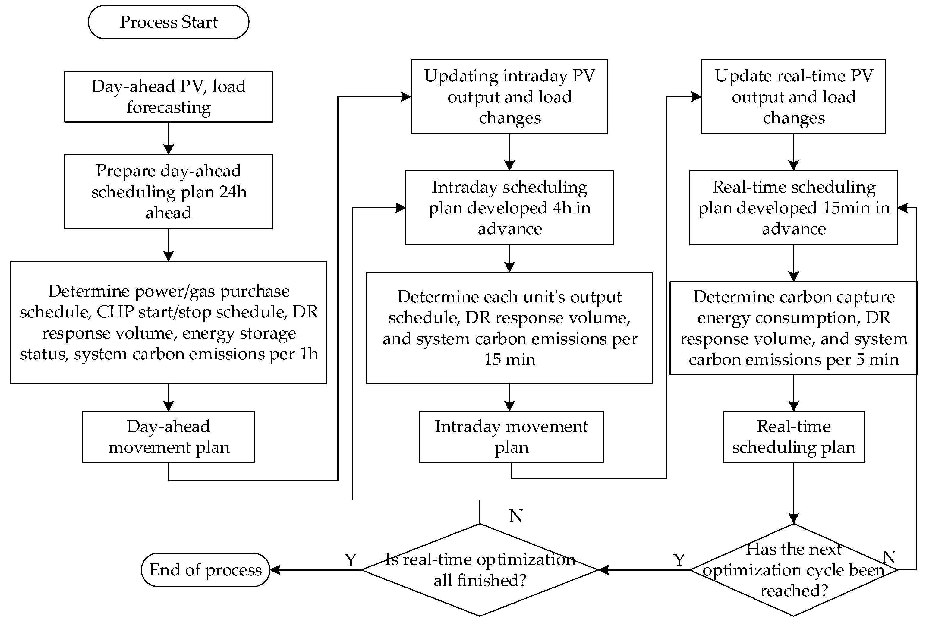
The real-time dispatch model is solved to obtain the following optimization results: power/gas purchase plan, CHP start–stop plan, each unit’s output plan, DR response, load status of energy storage devices, and system carbon emissions per 5 min during the real-time dispatch phase.

4.4. Solution Flow

The multi-timescale model proposed in this paper is a mixed-integer linear model, which can be solved layer by layer using the Gurobi solver 11.0.1. In this process, the scheduling results of the previous timescale will be used as an important reference basis for the scheduling plans of the subsequent timescales to ensure the consistency and optimization of the overall scheduling. Through this layer-by-layer solving approach, the system can more effectively respond to short-term and long-term power demand changes and achieve more accurate scheduling optimization. The specific solution process is shown in Figure 3.

5. Example Analysis

5.1. Basic Parameter Settings

In this paper, an optimal scheduling model for zero-carbon parks considering the flexible response of source–load bilaterals in multiple timescales is developed, and the model and algorithm are written using Matlab R2022a and run on a computer with a processor of AMD R9-7945HX and 8G of RAM. The validity and accuracy of the proposed method is verified through simulation of different scenarios and conditions.

In this paper, the park system shown in Figure 1 is used for arithmetic analysis. The energy prices in the system are shown in

Table A1. Energy prices.

Price Type	Time Interval	Parameters/(USD kW−1)
Time-of-use tariff	01:00–06:00	0.5
	07:00–13:00, 20:00–24:00	1.21
	14:00–19:00	0.73
Fixed purchase/sale price of electricity	01:00–24:00	0.8, 0.45
Fixed purchase price of gas	01:00–24:00	3.5

in Appendix A, the parameters of each device are shown in

Table A2. Basic equipment parameters.

Installations	Parameter Name	Parameter Value
PV unit	O&M cost per unit of power	${\lambda }^{\mathrm{PV}}=0.05$ (USD kW−1)
	Penalty cost per unit of power abandoned	${\delta }_{\mathrm{cur}}^{\mathrm{PV}}=0.5$ (USD kW−1)
CHP unit	Generation efficiency	${\eta }_{\mathrm{e}}^{\mathrm{CHP}}=0.4$
	O&M cost per unit of power	${\lambda }^{\mathrm{CHP}}=0.05$ (USD kW−1)
	Upper and lower limits of power generation/kW	$P_{\mathrm{e},\max }^{\mathrm{CHP}}=800,P_{\mathrm{e},\min }^{\mathrm{CHP}}=100$
	Maximum heat production power	$P_{\mathrm{h},\max }^{\mathrm{CHP}}=500$ kW
	Power generation at maximum heat production	$P_{\mathrm{e},0}^{\mathrm{CHP}}=160$ kW
	Upper and lower slopes	$k_1=-0.5,k_2=0.8$
	Start–sbottom costs	${\delta }^{\mathrm{CHP}}=50$ USD
	Climbing upper and lower limits	$\Delta P_{\max }^{\mathrm{CHP}}=100,\Delta P_{\min }^{\mathrm{CHP}}=10$
KLN unit	Generation efficiency	${\eta }_{\mathrm{e}}^{\mathrm{KLN}}=0.25$
	Maximum power	$P_{\mathrm{e},\max }^{\mathrm{KLN}}=200$ kW
	O&M cost per unit of power	${\lambda }^{\mathrm{KLN}}=0.05$ (USD kW−1)
Lithium bromide unit	Cooling efficiency	${\eta }_{\mathrm{c}}^{\mathrm{XHL}}=0.35$
	O&M cost per unit of power	${\lambda }^{\mathrm{XHL}}=0.05$ (USD kW−1)
GSHP unit	Heating/cooling efficiency	${\eta }_{\mathrm{h}}^{\mathrm{GSHP}}=0.8,{\eta }_{\mathrm{c}}^{\mathrm{GSHP}}=0.8$
	Maximum heating/cooling power/kW	$P_{\mathrm{h}}^{\mathrm{GSHP}}=71,P_{\mathrm{c}}^{\mathrm{GSHP}}=71$
	O&M cost per unit of power	${\lambda }^{\mathrm{GSHP}}=0.05$ (USD kW−1)
Carbon capture unit	Energy consumption factor	${\eta }^{\mathrm{ccs}}=0.65$
	Maximum power consumption	$P_{\mathrm{e},\max }^{\mathrm{CCS}}=100$ kW
	Upper and lower limits of trapping efficiency	${\eta }_{\max }^{\mathrm{CCS}}=0.65,{\eta }_{\min }^{\mathrm{CCS}}=0$
	O&M cost per unit of power	${\lambda }^{\mathrm{CCS}}=0.05$ (USD kW−1)
	Climbing upper and lower limits	$\Delta P_{\max }^{\mathrm{CCS}}=80,\Delta P_{\min }^{\mathrm{CCS}}=10$
ES unit	Charge and discharge efficiency	${\eta }_{\mathrm{ch}}^{\mathrm{ES}}=0.95,{\eta }_{\mathrm{dis}}^{\mathrm{ES}}=0.95$
	self-depletion rate	${\eta }_{\mathrm{loss}}^{\mathrm{ES}}=0.005$
	O&M cost per unit of power	${\lambda }^{\mathrm{ES}}=0.05$ (USD kW−1)
	Maximum charge/discharge power/kW	$P_{\mathrm{ch},\max }^{\mathrm{ES}}=100,P_{\mathrm{dis},\max }^{\mathrm{ES}}=100$
	Capacity upper and lower limits/kW	$S_{\max }^{\mathrm{ES}}=120,S_{\min }^{\mathrm{ES}}=12$
	Initial capacity/kW	$S_0^{\mathrm{ES}}=100$

, other relevant parameters are shown in

Table A3. Other relevant parameters.

Parameter Name	Parameter Value
Effective area of vegetation/km2	$S^{\mathrm{P}}=2.16$
Maximum power purchased and sold to the higher grid/kW	$P_{\mathrm{buy},\max }^{\mathrm{Grid}}=1000,P_{\mathrm{sell},\max }^{\mathrm{Grid}}=1000$
Maximum purchase of gas from the natural gas grid/cubic meter	$G_{\mathrm{buy},\max }^{\mathrm{Gas}}=500$
IDR load minimum response/kW	$\Delta P_{\mathrm{e},\min }^{\mathrm{IDR}}=50$
IDR load unit power compensation cost/(USD-kW−1)	${\delta }^{\mathrm{IDR}}=0.55$
Ideal room temperature/°C	$T^{\mathrm{iid}}=25$
Minimum permissible indoor comfort	$M_{\min }=0.8$
Temperature controlled load compensation cost/(USD-kW−1)	${\delta }^{\mathrm{TCL}}=0.1$
Direct heat transfer coefficient of building facades	${\eta }^{\mathrm{ew}}=24$
Heat transfer coefficient of internal walls of buildings	${\eta }^{\mathrm{iw}}=0.46$
Heat/cold energy and temperature conversion factor/(kW-°C−1)	${\eta }_{\mathrm{h}}^{\mathrm{T}}=12.5,{\eta }_{\mathrm{c}}^{\mathrm{T}}=12.5$
Coal/natural gas carbon emission factor/(kgCO2-kW−1)	$E_{\mathrm{c}}^{\mathrm{e}}=1.103,E_{\mathrm{g}}^{\mathrm{e}}=0.612$
Coal electric/thermal energy baseline factor/(kgCO2-kW−1)	${\kappa }_{\mathrm{c},\mathrm{e}}=0.7,{\kappa }_{\mathrm{c},\mathrm{h}}=0.2$

. The prediction curves for PV and all types of loads are generated based on real curves and follow normal distribution, and their prediction deviations on each timescale are shown in

Table A4. Uncertainty levels of predicted values at multiple timescales.

Section	PV/%	Carbon Credits	CEL/%	BFEL/%	BREL/%	BIEL/%	BFHL/%	BFCL/%	Room Temperature/%
Day-ahead	20	20	3	5	5	5	5	5	5
Intraday	5	5	1	3	3	3	3	3	3
Real-time	2	2	0.5	1	1	1	1	1	1

, and the source–load prediction curves are shown in Appendix A, Figure A1.

In this paper, it is considered that all carbon emissions generated by the system are borne by the park, and the benchmark price of stepped carbon trading is USD 0.25/kg, the length of the interval is 300 kg, and the price growth rate is 25%.

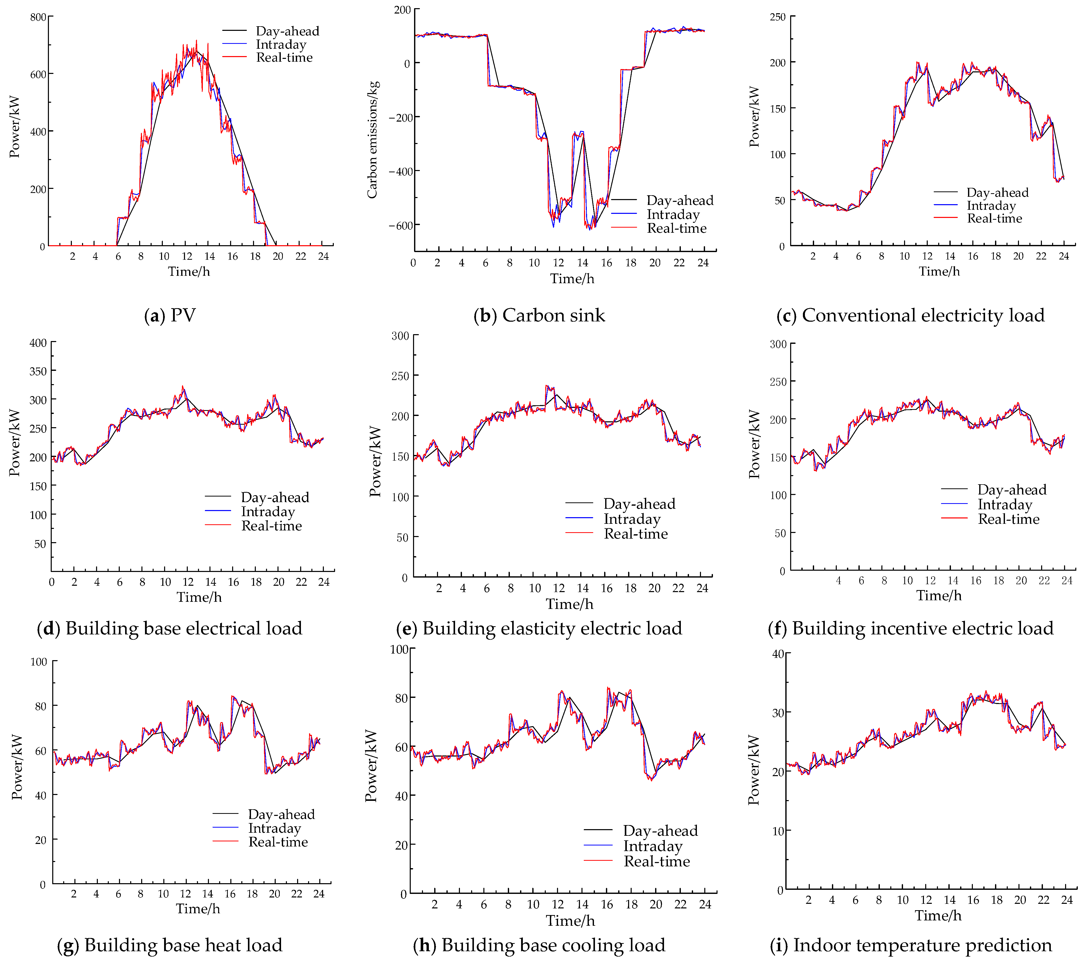
5.2. Analysis of the Results of the Previous Day’s Scheduling

The total system cost for the day-ahead scheduling scenario is USD 13,048, and the carbon trading cost is USD 1075, or 8.24% of the total cost. The day-ahead scheduling results of the system for electricity, heat, and cooling are shown in Figure 4.

The following observations can be noted from Figure 4:

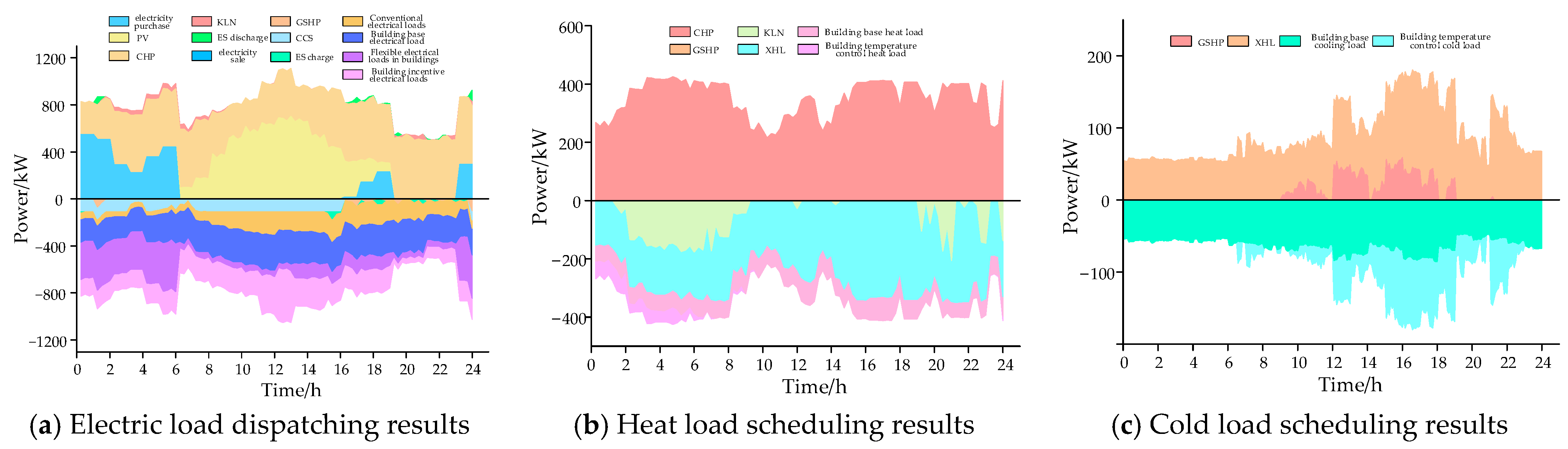
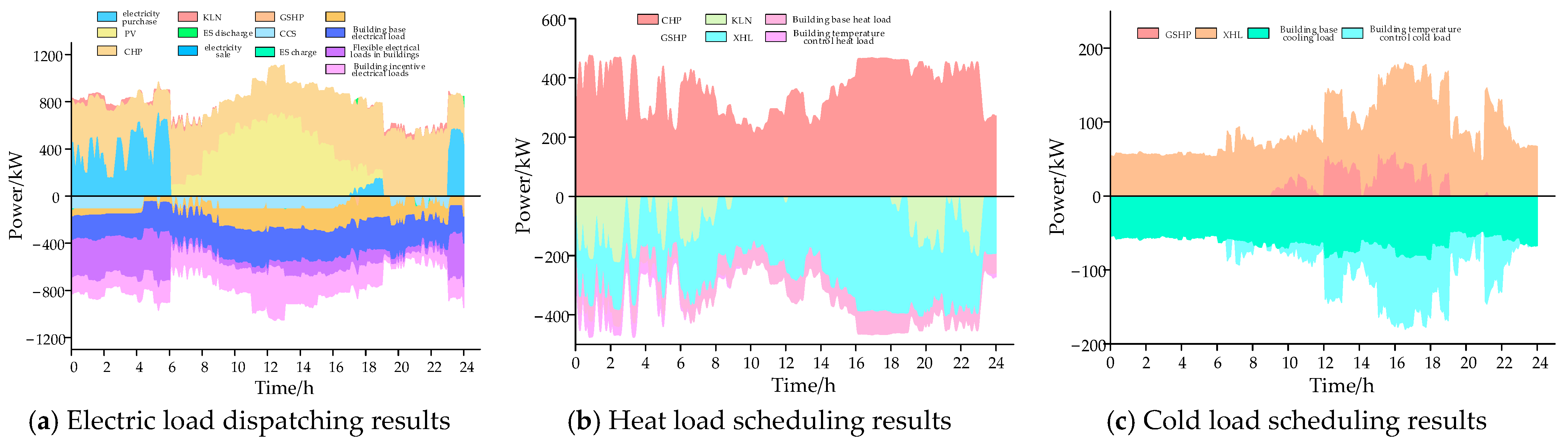
• The power supply of the park is supported by the higher grid, natural gas, and PV, with priority given to PV and the purchase of power from the higher grid when the price of electricity is low. Since PV is easily affected by light conditions, PV only supplies power to the park from 7 to 19 h. The rest of the time, the park is maintained by the higher grid and CHP. The KLN can not only recover electricity from flue gas waste heat, but can also absorb excess heat energy from CHP to generate electricity, which improves energy utilization efficiency. The energy storage device has a small capacity and only comes out when the unit’s ramp-up is restricted. The CCS operating in a flexible mode consumes more electrical energy during the 1–6 h period when the electricity price is low and the 8–16 h period when the PV is sufficient, separating CO₂ and sequestering it.
• The elastic electrical load of the building is strongly influenced by the electricity price, and mainly focuses on the 1~6 h and 14~19 h large amount of electricity consumption when the electricity price is lower or when the PV is sufficient. After the introduction of carbon potential correction coefficient, the resulting corrected tariff does not violate the peak and valley time division of time-sharing tariff on the overall trend, but on its benchmark, through the adjustment of the planned carbon potential and correction coefficient; the carbon potential changes brought about by the change of the energy composition structure are transmitted to the load side by the tariff signal. The load side, by changing its own electricity consumption hours, in turn affects the supply-side output, which in turn changes the energy composition structure and realizes the source–load synergistic interaction, with price curves and carbon potential curves as shown in Figure A2 in Appendix A. The building incentive electric loads are mainly concentrated in the period of 1~6 h when the price of electricity is lower and the period of 7~19 h when the PV is sufficient to use a large amount of electricity, which not only optimizes the operational burden of the park during the peak period, but also reduces the level of carbon emissions in the park.
• The heat supply of the park is supported by both CHP and GSHP, with priority given to the use of CHP to meet the heat demand, and shortfalls in heat made up by GSHP. XHL consumes a large amount of thermal energy to meet cooling demand. The building temperature control heat load flexibly adjusts its own heat use period in 1~6 h, 9 h, and 24 h, according to the actual indoor comfort requirement.
• The cold energy supply of the park is jointly supported by XHL and GSHP, with priority given to the use of XHL to meet the cold demand and the shortfall in cold energy made up by GSHP. The temperature-controlled cold load of the building is flexibly adjusted to its own cold period in 8 h and 11~23 h, according to the actual indoor comfort requirements.

As a result, in addition to flexibly adjusting complementary energy equipment to meet energy demand, the optimal scheduling model for zero-carbon parks also flexibly adjusts the demand side’s energy plan to achieve the effect of reducing carbon emissions. This allows the model to stimulate the source and load sides’ potential for reducing carbon emissions in a way that takes into account both the economy and low carbon. Finally, the model offers a scientific strategy and support for the promotion of the development of zero-carbon parks under the dual-carbon goal.

The methods and processes for analyzing the intraday and real-time phase scheduling results are generally similar to the day-ahead scheduling results, as shown in Figure A3 and Figure A4 of Appendix A, and will not be repeated.

5.3. Analysis of the Results of Different Scenarios

This work proposes a multi-timescale scheduling model and approach, whose efficacy is tested by comparing and analyzing the scheduling results of four distinct operating situations. The exact circumstances are as follows:

Scenario 1: Unit-variable condition operation, load-side-integrated demand response, and stepped carbon trading model (base model) are not considered.

Scenario 2: Considering only variable condition operation of the unit without considering load-side-integrated demand response and stepped carbon trading model.

Scenario 3: Considering unit-variable condition operation and load-side-integrated demand response without stepped carbon trading model.

Scenario 4: Multi-timescale scheduling strategy considering variable condition operation of units, load-side-integrated demand response, and stepped carbon trading.

Table 1. Simulation results of different scenarios.

Parameters	Scene 1	Scene 2	Scene 3	Scene 4
CRP/USD	12,802	12,125	11,035	10,620
CSS/USD	350	0	0	0
COM/USD	1306	1284	1031	1023
CCT/USD	/	/	/	1075
CCUR/USD	205	157	45	0
CIDR/USD	/	/	322	330
total cost/USD	14,663	13,566	12,433	13,048
carbon emissions/kg	1597	1542	1305	995

shows that, in comparison to Scenario 1, Scenario 2 introduces the unit-variable operating conditions operation model and flexibly adjusts the output plan according to the energy demand, which improves the rate of PV consumption and simultaneously lowers the total cost and carbon emissions by 7.48% and 3.44%, respectively. This indicates that Scenario 2 is more energy-efficient than Scenario 1 and verifies the validity of the unit-variable operating conditions operation model. In Scenario 3, the load-side-integrated demand response model is further introduced, based on the unit-variable operating condition operation model, to comply with the dispatch center’s instructions and flexibly adjust the load power plan to achieve the coordination and interaction of the source and load. In comparison to Scenario 2, the total cost and carbon emissions are reduced by 8.35% and 15.37%, respectively, proving the efficacy of the source–load bilateral flexible response model in this paper. To further achieve the target of reducing carbon emissions, a stepped carbon trading mechanism is introduced based on Scenario 3, which enhances the rate of photovoltaic consumption while reducing carbon emissions by 23.75%. This realizes the coupled response of park electricity and carbon, considering low carbon and the economy.

In summary, the model in this paper takes into account the operation of unit-variable operating conditions, load-side-integrated demand response, and a stepped carbon trading mechanism. It can also effectively reduce the total cost of the park and carbon emissions, as well as lessen the reliance on fossil fuels, by means of the source–load coordination and electric–carbon coupling mechanism. Finally, the model can improve PV power consumption.

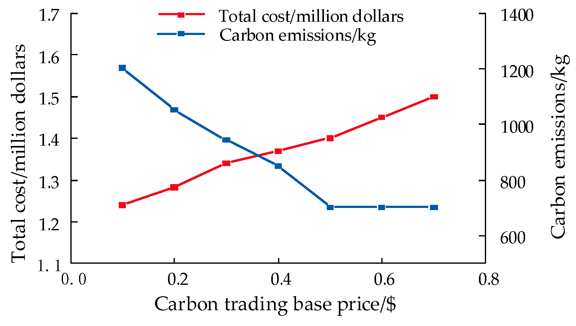
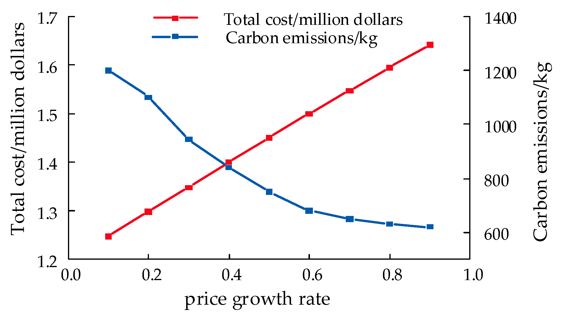
5.4. Analysis of Operational Results Under Different Carbon Trading Mechanism Parameters

This research analyzes the suggested scheduling model in depth to examine how carbon trading parameters affect system costs overall and carbon emissions [43].

Setting alternative carbon trading base prices with a step size of USD 0.1/kgCO₂, the duration of the carbon trading interim is 300 kg and the price inflation rate is 25%, the results are presented in Figure 5.

As demonstrated in Figure 5, the system’s overall cost gradually rises with the carbon trading base price before it falls below USD 0.5. In contrast, carbon emissions are comparatively lower because rising carbon trading base prices directly raise the cost per ton of carbon emissions, which increases the amount of money that goes toward carbon emissions. For economic reasons, the system takes steps to reduce carbon emissions. When the carbon trading base price exceeds USD 0.5, the system’s ability to reduce emissions has reached its maximum, and further increases in the carbon trading base price will have little or no effect on carbon emissions. However, when the emission reduction capacity has been maximized, the additional carbon emission costs faced by the system will not be reduced, but rather the total costs will continue to rise due to further increases in the base price.

Using a step size of 100 kgCO₂ to set various carbon trading intervals and investigate their effects on the system’s overall cost and carbon emissions, as well as a benchmark price of USD 0.25/kgCO₂ for step carbon trading and a 25% price growth rate, the findings are displayed in Figure 6.

As shown in Figure 6, the system’s carbon emissions are concentrated in the high step price bands when the carbon emission interval is less than 200 kg due to the step interval being too short, resulting in a high overall cost but comparatively low carbon emissions. The step interval widens and the system may trade carbon in lower price bands when the length of the carbon interval grows to 200–500 kg. This results in a drop in overall cost but an increase in carbon emissions. The lengthy step interval causes the system’s carbon emissions to be mostly distributed in the base price interval and the first step price interval when the carbon emission interval is above 500 kg. At this time, the cost of carbon trading tends to settle and the effect of extending the interval on carbon emissions progressively diminishes, slowing the rate of growth in the system’s overall cost as it gradually approaches equilibrium.

Using a step size of 10% to investigate the effects of varying carbon trading price growth rates on system overall costs and carbon emissions, Figure 7 displays the outcomes. The step carbon trading benchmark price is USD 0.25/kgCO₂, and the interval length is 300 kg.

Figure 7 illustrates how the price growth rate and total system cost are positively correlated, with the latter increasing gradually with the former. In the meantime, the system’s carbon emissions drastically drop when the price growth rate is less than 0.6 and gradually increase when it exceeds 0.6. This is due to the fact that, when the price growth rate is less than 0.6, the system is prompted to take proactive measures to reduce emissions. As a result, a greater portion of the total cost is accounted for by the carbon transaction cost, and the system optimizes unit output to control the total cost to reduce carbon emissions. However, when the price growth rate exceeds 0.6, the decline of carbon emissions slows down significantly, and the system’s emission reduction capability approaches its limit, making further reduction in carbon emissions difficult. Nonetheless, as the carbon trading price continues to rise, carbon trading costs continue to increase in the total cost, resulting in the overall system cost continuing to rise.

6. Conclusions

In order to solve the problem of large deviation between source–load prediction data and actual scheduling results and at the same time fully exploit the source–load flexibility resources to enhance the carbon reduction potential of the park, this paper establishes a zero-carbon park optimal scheduling model considering the source–load bilaterally flexible response in multiple timescales. Based on the example simulation, the main conclusions are as follows:

• In order to improve the park’s low-carbon economic benefits, a multi-temporal scheduling model is constructed that takes into account the response characteristics of flexibility resources and regulates source–load fluctuations. This approach is consistent with the operation of a zero-carbon park under source–load coordination and electricity–carbon coupling.
• The unit’s variable operating conditions, integrated demand response on the load side, and stepped carbon trading mechanism are all taken into account by the model in this paper, which fully utilizes the source–load coordination capability, increases the unit’s flexibility in operating under various loads and environmental conditions, and aids in the system’s more accurate controlling of carbon emissions.
• The scheduling outcomes of the system will be affected by various carbon trading characteristics. In addition, the scheduling model’s high degree of accuracy allows for more precise evaluation and optimization of the system’s scheduling strategy, which in turn enables the integration of renewable energy sources into demand response, lessens reliance on conventional energy sources, and produces a more precise and effective low-carbon operation.

References

1. Zhang, N.; Li, Z.; Zheng, X.; Liu, P. How Would Structural Change in Electricity and Hydrogen End Use Impact Low-Carbon Transition of an Energy System? A Case Study of China. Processes 2024, 12, 437. [Google Scholar] [CrossRef]
2. Long, X.; Liu, H.; Wu, T.; Ma, T. Optimal Scheduling of Source–Load Synergy in Rural Integrated Energy Systems Considering Complementary Biogas–Wind–Solar Utilization. Energies 2024, 17, 3066. [Google Scholar] [CrossRef]
3. Liu, G.; Wang, J.; Tang, Y. Evolution of research direction and application requirements of carbon emission factors in power grids. Grid Technol. 2024, 48, 12–28. [Google Scholar]
4. Meng, Q.; Zu, G.; Ge, L.; Li, S.; Xu, L.; Wang, R.; He, K.; Jin, S. Dispatching Strategy for Low-Carbon Flexible Operation of Park-Level Integrated Energy System. Appl. Sci. 2022, 12, 12309. [Google Scholar] [CrossRef]
5. Yang, Z.; Wang, X. Research on Low-Carbon Capability Evaluation Model of City Regional Integrated Energy System under Energy Market Environment. Processes 2022, 10, 1906. [Google Scholar] [CrossRef]
6. Li, Z.; Deng, F.; Zhu, Q.; Cao, L.; Jiang, Y. Do the Chinese Government’s Efforts to Make a Low-Carbon Industrial Transition Hinder or Promote the Economic Development? Evidence from Low-Carbon Industrial Parks Pilot Policy. Sustainability 2023, 15, 77. [Google Scholar] [CrossRef]
7. Zhang, J.; Liu, D.; Lyu, L.; Zhang, L.; Du, H.; Luan, H.; Zheng, L. Multi-Time-Scale Low-Carbon Economic Dispatch Method for Virtual Power Plants Considering Pumped Storage Coordination. Energies 2024, 17, 2348. [Google Scholar] [CrossRef]
8. Hua, P.; Wang, H.; Xie, Z.; Lahdelma, R. Integrated demand response method for heating multiple rooms based on fuzzy logic considering dynamic price. Energy 2024, 307, 132577. [Google Scholar] [CrossRef]
9. Le, S.; Zhang, Y.; Zhu, S.; Xie, S. Configuration-operation co-optimization of coal-fired power plants with carbon capture considering low-carbon demand response. Power Autom. Equip. 2024, 44, 278–286. [Google Scholar]
10. Wang, C.; Lu, Z.; Li, Y.; Zhang, J.; Kong, X. A collaborative planning approach for urban integrated energy systems considering hybrid energy storage and demand response. High Volt. Technol. 2024; in press. [Google Scholar]
11. Xia, R.; Dai, J.; Cheng, X.; Fan, J.; Ye, J.; Jia, Q.; Chen, S.; Zhang, Q. Demand Response of Integrated Zero-Carbon Power Plant: Model and Method. Energies 2024, 17, 3431. [Google Scholar] [CrossRef]
12. Ma, L.; Li, X.; Kong, X.; Yang, C.; Chen, L. Optimal participation and cost allocation of shared energy storage considering customer directrix load demand response. J. Energy Storage 2024, 81, 110404. [Google Scholar] [CrossRef]
13. Mugnini, A.; Ramallo-González, A.P.; Parreño, A.; Molina-Garcia, A.; Skarmeta, A.F.; Arteconi, A. Dynamic building thermal mass clustering for energy flexibility assessment: An application to demand response events. Energy Build. 2024, 308, 114011. [Google Scholar] [CrossRef]
14. Li, Y.; Han, M.; Yang, Z.; Li, G. Coordinating flexible demand response and renewable uncertainties for scheduling of community integrated energy systems with an electric vehicle charging station: A bi-level approach. IEEE Trans. Sustain. Energy 2021, 12, 2321–2331. [Google Scholar] [CrossRef]
15. Zhu, D.; Chen, W.; Guo, X.; Yin, X.; Liu, D. Hybrid time-scale scheduling strategy for wind power consumption by thermal storage electric heating and demand response. Chin. J. Electr. Eng. 2024; in press. [Google Scholar]
16. Li, X.; Zhang, R.; Bai, L.; Li, G.; Jiang, T.; Chen, H. Stochastic low-carbon scheduling with carbon capture power plants and coupon-based demand response. Appl. Energy 2018, 210, 1219–1228. [Google Scholar] [CrossRef]
17. Li, L.; Fan, S.; Xiao, J.; Zhou, H.; Shen, Y.; He, G. Fair trading strategy in multi-energy systems considering design optimization and demand response based on consumer psychology. Energy 2024, 306, 132393. [Google Scholar] [CrossRef]
18. Cheng, M.; Niu, W.; Hu, J.; Wang, Z.; Chen, J.; Lin, C. Construction mode optimal selection method for intelligent sensing system in zero-carbon parks. J. Eng. 2023, 2023, e12326. [Google Scholar] [CrossRef]
19. Hu, Y.; Xie, T.; Chi, N.; Yang, Y. Design of energy big data and carbon emission monitoring system based on perceptron model in the context of carbon neutral and carbon peaking. Appl. Math. Nonlinear Sci. 2024, 9. [Google Scholar] [CrossRef]
20. Zahedmanesh, A.; Verbic, G.; Rajarathnam, G.; Weihs, G.F.; Shikata, K.; Matsuda, N.; Abbas, A. Optimal design of greenfield energy hubs in the context of carbon neutral energy supply. Energy 2024, 305, 132284. [Google Scholar] [CrossRef]
21. Asano, H.; Ishii, H.; Takano, H. Distributed Energy Resource Integration for Carbon Neutral Power Systems: Market-Based Approaches to Ancillary Services and Microgrid Operation. IEEJ Trans. Electr. Electron. Eng. 2024, 19, 598–607. [Google Scholar] [CrossRef]
22. Wang, L.; Zhang, S.; Fu, Y.; Liu, M.; Liu, J.; Yan, J. Heat–power decoupling for the CHP unit by utilizing heat storage in the district heating system integrated with heat pumps: Dynamic modeling and performance analysis. Energy 2024, 306, 132485. [Google Scholar] [CrossRef]
23. Ding, X.; Yang, Z.; Zheng, X.; Zhang, H.; Sun, W. Effect of decision-making principle on P2G–CCS–CHP complementary energy system based on IGDT considering energy uncertainty. Int. J. Hydrogen Energy 2024, 81, 986–1002. [Google Scholar] [CrossRef]
24. Liu, X. Multiple time-scale economic dispatching strategy for commercial building with virtual energy storage under demand response mechanism. Int. J. Energy Res. 2021, 45, 16204–16227. [Google Scholar] [CrossRef]
25. Wang, L.; Ren, X.; Ma, Y.; Liu, Z.; Dong, W.; Ni, L. Optimal low-carbon scheduling of integrated energy systems considering stepped carbon trading and source-load side resources. Energy Rep. 2024, 12, 3145–3154. [Google Scholar] [CrossRef]
26. Yan, X.; Wang, L.; Fang, M.; Hu, J. How Can Industrial Parks Achieve Carbon Neutrality? Literature Review and Research Prospect Based on the CiteSpace Knowledge Map. Sustainability 2023, 15, 372. [Google Scholar] [CrossRef]
27. Feng, J.; Yan, J.; Yu, Z.; Zeng, X.; Xu, W. Case study of an industrial park toward zero carbon emission. Appl. Energy 2018, 209, 65–78. [Google Scholar] [CrossRef]
28. Cheng, J.; Wang, L.; Pan, T. Optimized configuration of distributed power generation based on multi-stakeholder and energy storage synergy. IEEE Access 2023, 11, 129773–129787. [Google Scholar] [CrossRef]
29. Cheng, Y.; Zhang, N.; Wang, Y.; Yang, J.; Kang, C. Modeling carbon emission flow in multiple energy systems. IEEE Trans. Smart Grid 2018, 10, 3562–3574. [Google Scholar] [CrossRef]
30. Xu, D.; Xiang, S.; Bai, Z.; Wei, J.; Gao, M. Optimal multi-energy portfolio towards zero carbon data center buildings in the presence of proactive demand response programs. Appl. Energy 2023, 350, 121806. [Google Scholar] [CrossRef]
31. Chu, X.; Fu, L.; Liu, Q.; Yu, S. Optimal allocation method of oxygen enriched combustion-carbon capture low-carbon integrated energy system considering uncertainty of carbon-source-load. Int. J. Electr. Power Energy Syst. 2024, 162, 110220. [Google Scholar] [CrossRef]
32. Li, J.; Xu, L.; Zhang, Y.; Kou, Y.; Liang, W.; Bieerke, A.; Yuan, Z. Economic Dispatch of Integrated Energy Systems Considering Wind–Photovoltaic Uncertainty and Efficient Utilization of Electrolyzer Thermal Energy. Processes 2024, 12, 1627. [Google Scholar] [CrossRef]
33. Ramezani, R.; Di Felice, L.; Gallucci, F. A review on hollow fiber membrane contactors for carbon capture: Recent advances and future challenges. Processes 2022, 10, 2103. [Google Scholar] [CrossRef]
34. Zhang, X.; Chen, S.; Wei, Z.; Liang, Z. Low-carbon planning of integrated energy systems in parks taking into account generalized energy storage. Power Autom. Equip. 2024, 44, 40–48. [Google Scholar]
35. Zhao, H.; Miao, S.; Li, C.; Zhang, D.; Tu, Q. Optimized operation strategy of integrated energy system in a park considering coupled response characteristics of cooling, heating and power demand. Chin. J. Electr. Eng. 2022, 42, 573–589. [Google Scholar]
36. Li, M.; Meng, X.; Wang, J.; Qi, C.; Ji, X.; Wang, H. Optimal Scheduling Strategy of Park Integrated Energy System Considering Ladder Carbon Trading Mechanism and Demand Response. In Proceedings of the 2023 8th Asia Conference on Power and Electrical Engineering (ACPEE), Tianjin, China, 14–16 April 2023; pp. 1390–1394. [Google Scholar]
37. Liang, T.; Chai, L.; Tan, J. Dynamic optimization of an integrated energy system with carbon capture and power-to-gas interconnection: A deep reinforcement learning-based scheduling strategy. Appl. Energy 2024, 367, 123390. [Google Scholar] [CrossRef]
38. Cai, F.; Wen, Z.; Jia, X. Multi-Time Scale Low-Carbon Optimization of IES Considering Demand Response of Multi-Energy. In Proceedings of the 2022 IEEE Conference on Telecommunications, Optics and Computer Science (TOCS), Dalian, China, 11–12 December 2022; pp. 793–799. [Google Scholar]
39. Zhu, G.; Gao, Y. Multi-objective optimal scheduling of an integrated energy system under the multi-time scale ladder-type carbon trading mechanism. J. Clean. Prod. 2023, 417, 137922. [Google Scholar] [CrossRef]
40. Dai, R.; Zhang, X.; Zou, H. Two-Stage Distributed Robust Optimal Allocation of Integrated Energy Systems under Carbon Trading Mechanism. Processes 2024, 12, 1044. [Google Scholar] [CrossRef]
41. Xie, T.; Wang, Q.; Zhang, G.; Zhang, K.; Li, H. Low-Carbon Economic Dispatch of Virtual Power Plant Considering Hydrogen Energy Storage and Tiered Carbon Trading in Multiple Scenarios. Processes 2024, 12, 90. [Google Scholar] [CrossRef]
42. Cao, W.; Yu, J.; Xu, M. Optimization Scheduling of Virtual Power Plants Considering Source-Load Coordinated Operation and Wind–Solar Uncertainty. Processes 2024, 12, 11. [Google Scholar] [CrossRef]
43. Wu, M.; Xu, J.; Li, Y.; Zeng, L.; Shi, Z.; Liu, Y. Low carbon economic dispatch of integrated energy systems considering life cycle assessment and risk cost. Int. J. Electr. Power Energy Syst. 2023, 153, 109287. [Google Scholar] [CrossRef]
Figure 1. Structure of zero-carbon park.
Processes 12 02850 g001
Figure 2. Multi-timescale low-carbon economy scheduling framework.
Processes 12 02850 g002
Figure 3. Multi-timescale model solution flow.
Processes 12 02850 g003
Figure 4. Day-ahead scheduling results for different energy loads. (a) Electric load dispatching results; (b) heat load scheduling results; (c) cold load scheduling results.
Processes 12 02850 g004
Figure 5. Impact of carbon trading base price on total costs and carbon emissions.
Processes 12 02850 g005
Figure 6. Impact of carbon trading bands on total costs and carbon emissions.
Processes 12 02850 g006
Figure 7. Impact of price growth rates on total costs and carbon emissions.
Processes 12 02850 g007