Improving the Classification Efficiency of an ANN Utilizing a New Training Methodology


Computer & Informatics Engineering Department, Technological Educational Institute of Western Greece, GR 263-34 Antirion, Greece
Informatics 2019, 6(1), 1; https://doi.org/10.3390/informatics6010001
Submission received: 31 October 2018
/
Revised: 10 December 2018
/
Accepted: 24 December 2018
/
Published: 28 December 2018
(This article belongs to the Special Issue Advances in Randomized Neural Networks)
Abstract
:In this work, a new approach for training artificial neural networks is presented which utilises techniques for solving the constraint optimisation problem. More specifically, this study converts the training of a neural network into a constraint optimisation problem. Furthermore, we propose a new neural network training algorithm based on the L-BFGS-B method. Our numerical experiments illustrate the classification efficiency of the proposed algorithm and of our proposed methodology, leading to more efficient, stable and robust predictive models.
1. Introduction
Artificial neural networks constitute distributed processing systems, comprised of densely interconnected, adaptive processing units, characterised by an inherent propensity for learning from experience and also discovering new knowledge. The excellent capability of self-learning and self-adapting of these learning systems has established them as powerful tools for pattern recognition and as vital component of many classification systems. Thus, they have been extensively studied and widely used in many applications of artificial intelligence (see [1,2,3,4,5,6,7] and the references there in). In the literature, although many different models and have been proposed, the Multi-Layer Perceptron (MLP) is the most commonly and widely used in a variety of applications. The operation of an MLP is usually based on the following equations:
where is the sum of its weighted inputs for the j-th node in the l-th layer , are the weights from the i-th neuron at the layer to the j-th neuron at the l-th layer, is the bias of the j-th neuron at the l-th layer, is the output of the j-th neuron that belongs to the l-th layer and is the j-th neuron activation function.
The problem of training an MLP is an incremental adaptation of connection weights which propagate information contained in the examples of the training set, between simple processing units called neurons [8]. More mathematically, the problem of training an MLP can be formulated as the minimisation of an error function E defined by the sum of square differences over all examples of the training set, namely
where is the actual output of the j-th neuron that belongs to the L-th (output) layer, is the number of neurons of the output layer, is the desired response at the j-th neuron of the output layer at the input pattern p and P represents the total number of patterns used in the training set. To simplify the formulation of the above equations, let us use a unified notation for the weights. To this end, for an MLP with n weights, let be a column weight vector with components and be an optimal weight vector defined by the solution of
Gradient-based training algorithms are usually applied to deal with this problem (2) by generating a sequence of weights utilising the following iterative formula
where k is the current iteration usually called epoch, is a given starting point, is a stepsize (or learning rate) with and is a descent search direction. Furthermore, the gradient can be easily obtained by means of back propagation of errors through the network layers.
Since the appearance of backpropagation [8], a variety of approaches were suggested for improving the efficiency of the minimisation error process. It is worth noting that the optimisation problem (2) is significantly challenging since its dimensionality is usually high and the corresponding nonconvex multimodal error function possesses multitudes of local minima and has broad flat regions adjoined with narrow step ones. Therefore, several methods based on the well established unconstrained optimisation theory have been suggested which utilize second order derivative related information, such as limited memory quasi-Newton methods [9,10,11] and conjugate gradient methods [12,13,14]. Another interesting approach for improving the generalisation efficiency of a neural network was based on the adaptation of nonmonotone learning strategies, exploiting the accumulated information with regard to the most recent values of the error function. Along this line, Peng and Magoulas [15,16,17,18] and Livieris and Pintelas [19] proposed nonmonotone training algorithms which possess strong convergence properties and also have good classification performance. Karras and Perantonis [20,21] considered incorporating knowledge in the form of constraints in neural networks learning process and presented a Lagrange multiplier approach for the minimisation of the error function (1) in order to improve convergence. The advantage of their proposed method was that the weights updates in two successive epochs are highly aligned, therefore, avoiding zig-zag trajectories in the parameter space and improving the speed of convergence.
After a neural network is successfully trained, its classification accuracy is depended on its architecture, but mostly on the values of its weights. Nevertheless, since there are no restrictions and limitations on the weights during the training process, a small number of weights may significantly affect the output of the network. In other words, in case some of the weights have large values, they dominate and sometimes determine the neural network’s output; therefore, degrading the classification efficiency of the network since only some of the inputs of the network will be efficiently explored.
The major novelty of this work is that the problem of efficiently training an ANN is re-formulated as a constrained optimisation problem by defining bounds on the weights. More specifically, in order to avoid the degradation of the classification accuracy, we consider the training problem as follows
where the vectors and denote the lower and upper bounds on the weights of the optimisation problem, respectively. Our basic aim and motivation is focused on defining the weights in the trained network in more uniform way, by restricting them from taking large values. In this case all the inputs will be efficiently explored for improving the classification ability of the network. Furthermore, in order to evaluate the efficacy and the efficiency of our proposed methodology, we propose a new weight constrained neural network training algorithm which is based on the L-BFGS-B method. The rationale behind this selection is based upon the fact that limited memory BFGS constitutes an elegant choice for efficiently training neural networks due to their numerical efficiency and their very low memory requirements [22]. Our preliminary numerical experiments illustrate the classification efficiency of the proposed algorithm and our proposed methodology.
The remainder of this paper is organized as follows: Section 2 presents the proposed weight constrained neural network training algorithm and Section 3 presents the numerical experiments using the performance profiles Dolan and Morè [23]. Finally, Section 4 presents the discussion, our concluding remarks and our proposals for future research.
Notations. Throughout this paper, the gradient of the error function is indicated by and the vectors and represent the evolutions of the current point and of the error function gradient between two successive iterations.
2. Weight Constrained Neural Network Training Algorithm
In this section, we present the proposed neural network training algorithm, which is based on the L-BFGS-B method.
L-BFGS-B [24] constitutes one of the most successful and efficient large-scale bound-constrained optimisation methods. More analytically, L-BFGS-B is a limited-memory algorithm which minimizes a nonlinear function subject to simple bounds on the variables, by efficiently combining L-BFGS updates with a gradient-projection strategy. In contrast to the traditional BFGS method which stores a dense approximation, the L-BFGS-B stores only a small number, say m, of vectors which implicitly describe the approximation. Thus, this moderate requirement of memory makes L-BFGS-B well suitable especially for the optimisation problems with a large number of variables.
At each iteration of the L-BFGS-B algorithm, the error function E is approximated by a quadratic model at a point , that is
where and the Hessian approximation is defined as follows. Let , then given the set of correction vector pairs for , we define the matrices
The Hessian approximation (in compact form) resulting from updates to the basic matrix is given by
where is a positive scalar and and are the matrices
Subsequently, the algorithm approximately minimizes subject to the feasible domain utilizing the gradient projection method to find a set of active bounds, followed by a minimisation of treating those bounds as equality constraints. In more detail, this procedure is performed in three stages: (1) the computation for the generalized Cauchy point; (2) the subspace minimisation; and (3) the line search.
Stage I: Cauchy point computation. The basic objective of this stage is to compute the generalized Cauchy point . This is defined as the local minimum of quadratic approximation of the error function, starting from the current point , on the path defined by the projection of the steepest descent direction on the feasible domain D, that is
Notice that the variables whose value at is at lower or upper bound, comprising the active set , are held fixed.
Stage II: Subspace minimisation. After the generalized Cauchy point is obtained, the quadratic function (5) is minimized for the free variables in i.e. variables whose values are not at lower or upper bound. To solve this minimizing problem, a direct primal method [24] is utilized to find the minimizer , by using the following formulation:
Notice that the feasibility domain is reduced at a subspace of the feasibility domain
by considering as free variables, the variables that are not fixed on limits while the rest variables are fixed on their boundary value obtained during the Cauchy point calculation stage.
Step III: Line search. After an approximate solution of this problem has been obtained, we compute the new iterate by a line search along which satisfies the strong Wolfe line search conditions, that is
with . Summarizing the above discussion, we present a high level description of the proposed Weight Constrained Neural Network (WCNN) training algorithm.
| Algorithm 1: Weight Constrained Neural Network Training Algorithm |
|
It is worth noticing that since the Algorithm 1 is implemented with a line search which satisfies the strong Wolfe conditions, every Hessian approximation is positive definite. Therefore, the solution of the quadratic problem (7) defines a descent direction for the error function [24]. The significance of the sufficient descent property is highlighted in [12,13,19] in order to avoid the usually inefficient restarts which degrade the overall efficiency and robustness of the minimisation process.
3. Experimental Analysis
In this section, we will present experimental results in order to evaluate the performance of the proposed neural network training algorithm in six famous classification problems acquired by the UCI Repository of Machine Learning Databases [25]: the breast cancer problem, the Australian credit card problem, the diabetes problem, the Escherichia coli problem, the Coimbra problem and the SPECT heart problem. Table 1 presents a brief description of each datasets’ structure i.e., number of attributes (#Features) and the number of instances (#Instances) and the network architectures and total number of weights for each problem.
All MLPs had logistic activation functions and received the same sequence of input patterns. Moreover, the weights were initiated using the Nguyen-Widrow method [26]. The classification accuracy of each algorithm was evaluated using the standard procedure called stratified k-fold cross-validation. The implementation code was written in Matlab 7.6 and the simulations have been carried out on a PC (2.66GHz Quad-Core processor, 4Gbyte RAM) running Linux operating system while the results have been averaged over 300 simulations.
Our experimental analysis was obtained by conducting a two phase procedure: In the first phase, the classification performance of the proposed algorithm WCNN was evaluated against the classical training method L-BFGS. The rationale for the selection of these algorithms is based upon the fact that L-BFGS-B is a substantial extension of the classical L-BFGS [22] for constrained optimisation problems; hence, both methods require the same information per iteration. In the second phase, we evaluate the performance of WCNN against the state-of-the-art neural network training algorithms Resilient backpropagation [27], scaled conjugate gradient [14] and Levenberg-Marquardt training algorithm [28].
The cumulative total for a performance metric over all simulations does not seem to be too informative, since a small number of simulations tend to dominate these results. For this reason, we utilize the performance profiles of Dolan and Morè [23] relative to the performance metrics: accuracy and F1-score, to present perhaps the most complete information in terms of robustness, efficiency and solution quality. The use of performance profiles eliminates the influence of a small number of simulations on the benchmarking process and the sensitivity of results associated with the ranking of solvers [23]. The performance profile plots the fraction P of simulations for which any given method is within a factor of the best training method.
More specifically, assume that there exist solvers and problems for each solver s and problem p, Requiring a baseline for comparisons, Dolan and Morè compared the performance (based on a metric) by solver s on problem p with the best performance by any solver on this problem; namely, using the performance ratio
The performance of solver s on any given problem might be of interest, but we would like to obtain an overall assessment of the performance of the solver. Next, the function was the (cumulative) distribution function for the performance ratio is defined by
where is the set of all problems. Notice that the performance profile for a solver was a non-decreasing, piecewise constant function, continuous from the right at each breakpoint [23].
In other words, the performance profile plots the fraction P of problems for which any given algorithm is within a factor of the training algorithm. The horizontal axis of each figure gives the percentage of the simulations for which a training algorithm achieved the best performance (efficiency). Regarding the above rules and discussion, we can conclude that one solver whose performance profile plot lies on top right, outperforms the rest of the solvers.
3.1. Performance Evaluation Against L-BFGS Algorithm
Next, we briefly describe each classification problem and present the performance comparison between the proposed algorithm WCNN and L-BFGS training algorithm. The curves in the following figures have the following meaning
- “WCNN1” stands for Algorithm 1 with bounds on the weights .
- “WCNN2” stands for Algorithm 1 with bounds on the weights .
- “WCNN3” stands for Algorithm 1 with bounds on the weights .
- “L-BFGS” stands for the limited-memory BFGS.
WCNN and L-BFGS were evaluated using and as in [22] and were implemented with the same line search [24] with and .
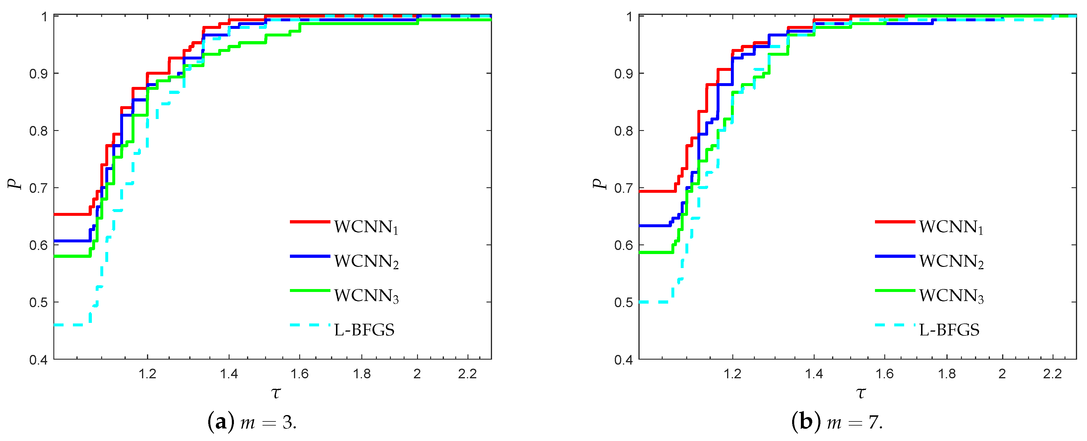
3.1.1. Breast Cancer Classification Problem
The first benchmark concerns the diagnosis of breast cancer malignancy. The data have been collected from 683 patients from the University of Wisconsin each having 9 attributes and a class label (malignant or benign tumor). We have used neural networks with 2 hidden layers of 4 and 2 neurons respectively, as suggested in [12]. The stopping criterion is set to within the limit of 2000 epochs and all networks were tested using 10-fold cross validation.
Figure 1 and Figure 2 present the performance profiles for the breast cancer classification problem, based on accuracy and F1-score, respectively. Firstly, it is worth noticing that all versions of WCNN exhibited better performance than L-BFGS, regarding both performance metrics. Therefore, the bounds on the weights, substantially led to the development of trained neural networks with improved classification accuracy. Regarding the performance of the proposed algorithm, WCNN1 illustrates the best performance in terms of generalisation ability, followed by WCNN2 and WCNN3. Moreover, the interpretation of Figure 1 and Figure 2 report that tighter the bounds on the weights, the more efficient the resulting classification performance will be (in most cases).
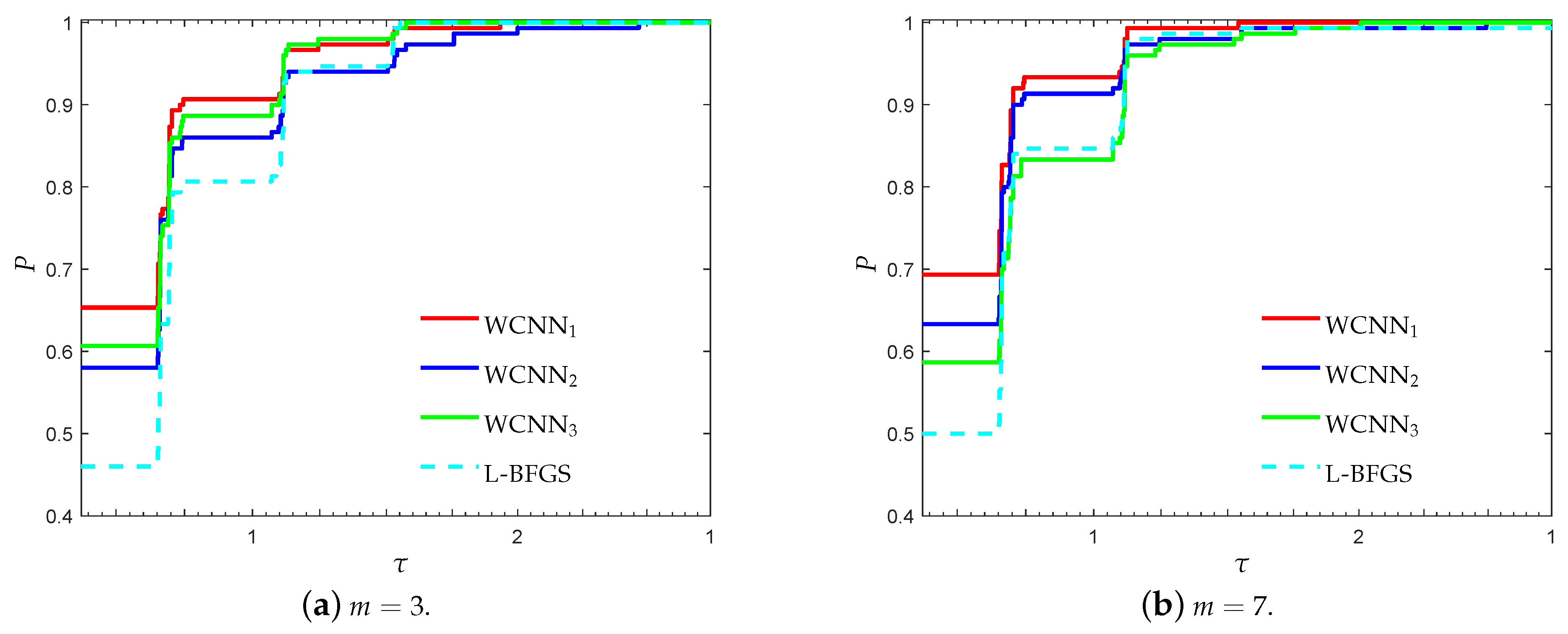
3.1.2. Australian Credit Card Classification Problem
The Australian credit approval dataset contains all the details about credit card applications. This dataset is interesting because the data varies and has mixture of attributes which is continuous, nominal with small numbers of values and nominal with larger numbers of values. We have used neural networks with two hidden layers with 16 and 8 neurons and an output layer of 2 neurons [12]. The termination criterion is set to within the limit of 1000 epochs and all networks were tested using 10-fold cross validation.
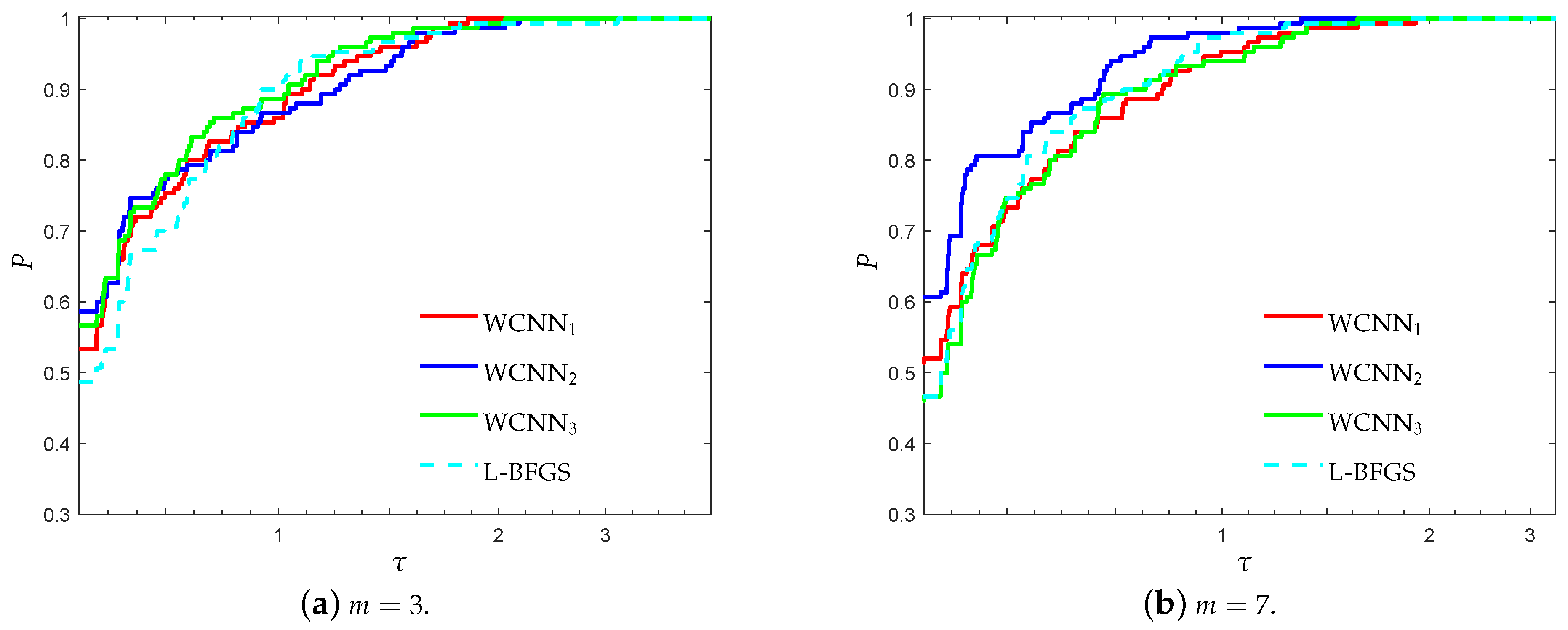
Figure 3 and Figure 4 illustrate the performance profiles for the Australian credit card classification problem, investigating the efficiency and robustness of each training method. Similar observations can be made with the previous benchmark. WCNN1 outperforms all other training methods, since its curves lie on the top, relative to each value of parameter m. More specifically, WCNN1 for and reported 65%, and 69.3% of simulations with the highest classification accuracy, respectively; while L-BFGS reported only 46% and 50%, in the same situations. Summarizing, we conclude that the tighter the bounds get, the higher the chance for good generalisation performance (i.e., the classification ability of the neural network will he higher).
3.1.3. Diabetes Classification Problem
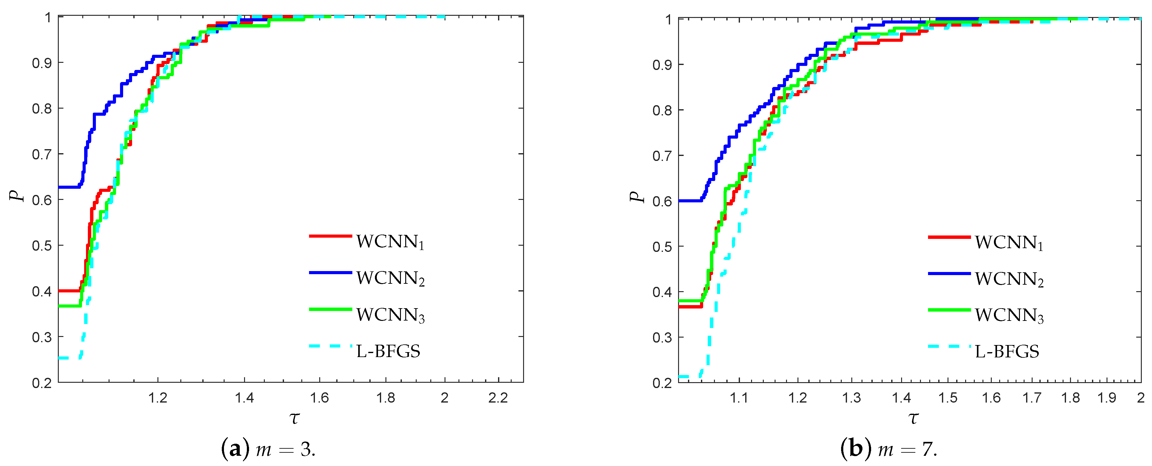
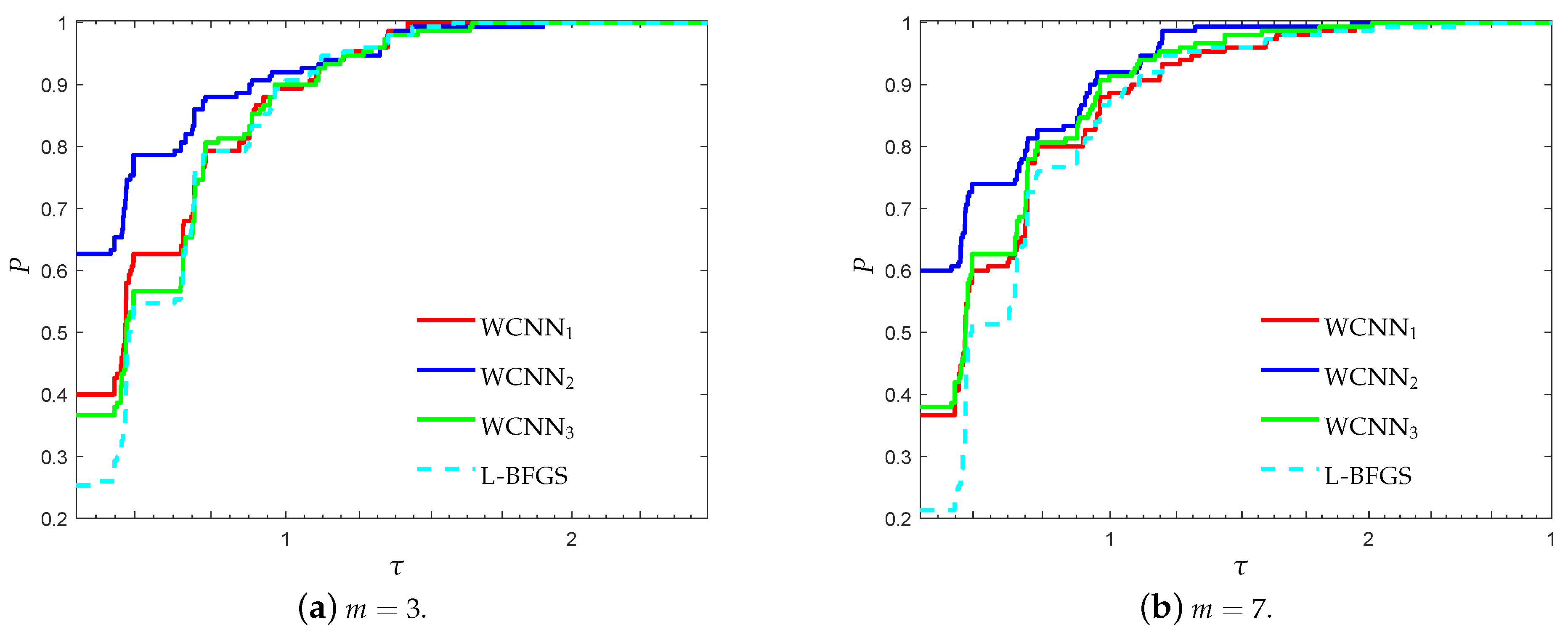
The aim of this real-world classification task is to decide when a Pima Indian female is diabetes positive or not. The data of this benchmark consists of 768 different patterns each of them having 8 features of real continuous values and a class label (diabetic positive or not). We have used neural networks with 2 hidden layers of 4 neurons each and an output layer of 2 neurons [12]. The termination criterion is set to within the limit of 2000 epochs and all networks were tested using 10-fold cross validation [29].
Figure 5 and Figure 6 illustrate the performance profiles for the diabetes classification problem, relative to each performance metric. WCNN2 exhibits the best probability of being the optimal solver in terms of efficiency and robustness, outperforming all training methods, followed by WCNN1 and WCNN3 which exhibited almost similar performance. More specifically, WCNN2 reported 62.6% and 60% of simulations with the highest classification accuracy for and , respectively, while L-BFGS presented the worst performance among all training methods. In general, the interpretation of Figure 5 and Figure 6 reveal that the bounds on the weights increased the overall classification accuracy, in most cases. Nevertheless, in contrast to the previous benchmarks, in case the bounds are too tight, this substantially did not benefit much the classification performance of the networks.
3.1.4. Escherichia coli Classification Problem
This problem is based on a drastically imbalanced data set of 336 patterns and concerns the classification of the E. coli protein localisation patterns into eight localisation sites. E. coli, being a prokaryotic gram-negative bacterium, is an important component of the biosphere. Three major and distinctive types of proteins are characterized in E. coli: enzymes, transporters and egulators. The largest number of genes encodes enzymes (34%) (this should include all the cytoplasm proteins) followed by the genes for transport functions and the genes for regulatory process (11.5%) [30]. The network architectures consists of one hidden layer with 16 neurons and an output layer of 8 neurons [31]. The termination criterion is set to within the limit of 2000 epochs and all neural networks were tested using four-fold cross-validation.
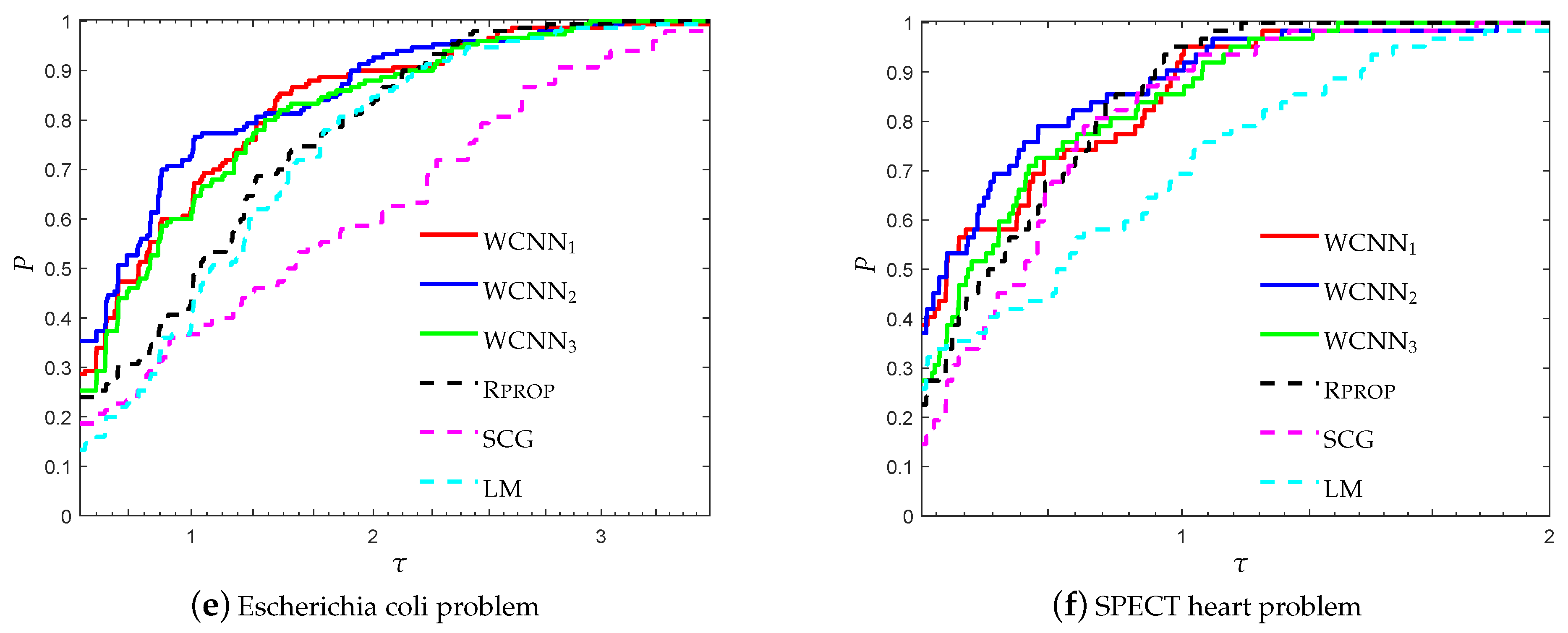
Figure 7 and Figure 8 present the performance profiles for the Escherichia coli classification problem, based on the performance metrics accuracy and F1-score, respectively. Similar observations can be made with the previous benchmarks. Firstly, it is worth noticing that in most cases the bounds on the weights, lead to the training of neural networks with higher classification accuracy. More specifically, WCNN1, WCNN2 and WCNN3 exhibited better generalisation performance than the classical training method L-BFGS. Furthermore, Figure 7 and Figure 8 report that WCNN2 exhibits the best performance in terms of classification ability, followed by WCNN1 and WCNN3.
3.1.5. Coimbra Classification Problem
This dataset is comprised of ten predictors, all quantitative, and a binary dependent variable, indicating the presence or absence of breast cancer [32]. The predictors are anthropometric data and parameters which can be gathered in routine blood analysis. Prediction models based on these predictors, if accurate, can potentially be used as a biomarker of breast cancer. The network architectures consists of two hidden layers of five and two neurons, respectively, and an output layer of two neurons. The termination criterion is set to within the limit of 1000 epochs and all neural networks were tested using ten-fold cross-validation.
Figure 9 and Figure 10 illustrate the performance profiles for the Coimbra classification problem, investigating the classification efficiency of each training method. WCNN2 exhibited the best performance, since its curves lie on the top, relative to each value of parameter m, followed by WCNN1 and WCNN3. It is worth noticing that WCNN2 for and reported 62% and 55.3% of simulations with the highest classification accuracy, respectively; while L-BFGS exhibited the worst performance, reporting only 32% and 33.3%, in the same situations. Although that in most cases WCNN appears to train neural networks with higher classification accuracy on average; however if the bounds are too tight, this substantially did not benefit much the generalisation ability of the networks.
3.1.6. SPECT Heart Classification Problem
This dataset contains data instances derived from cardiac Single Proton Emission Computed Tomography (SPECT) images from the University of Colorado. This is also a binary classification task, where patients heart images are classified as normal or abnormal. The class distribution has 55 instances of the abnormal class (20.6%) and 212 instances of the normal class (79.4%). From them there have been selected 80 instances for the training process and the remainder 187 for testing the neural networks generalisation capability [25]. The network architecture consists of two hidden layers with 16 and 8 neurons, respectively, and an output layer of two neurons [12]. The training goal was set to and the maximum number of epochs was set to 1000 as in [12].
Figure 11 and Figure 12 report the performance profiles for the SPECT heart classification problem, relative to the values of parameter m. For , WCNN1, WCNN2, WCNN3 exhibited similar performance, with WCNN3 presenting slightly better results. For , WCNN2 exhibits the best probability of being the optimal solver, followed by WCNN1 and WCNN3 which exhibited similar performance. Furthermore, L-BFGS presented the worst performance compared against all training methods. Therefore, the interpretation of Figure 11 and Figure 12 demonstrate that application of the bounds on the weights of the neural network, increased the overall classification accuracy, in most cases. Nevertheless, by comparing the performance of all versions of the proposed algorithm, we are able to conclude that in case the bounds are too tight this will not substantially benefit much the classification performance.
3.2. Performance Evaluation against State-of-the-Art Training Algorithms
In the sequel, we evaluate the performance of the proposed neural network training algorithm WCNN against state-of-the-art training algorithms, i.e. Resilient backpropagation, scaled conjugate gradient and Levenberg-Marquardt training algorithm which were utilized with their default parameter settings. The curves in the following figures have the following meaning
- “WCNN1” stands for Algorithm 1 with and bounds on the weights .
- “WCNN2” stands for Algorithm 1 with and bounds on the weights .
- “WCNN3” stands for Algorithm 1 with and bounds on the weights .
- “Rprop” stands for Resilient backpropagation.
- “SCG” stands for scaled conjugate gradient.
- “LM” stands for Levenberg-Marquardt training algorithm.
Figure 13 present the performance profiles based on accuracy of WCNN, Rprop, SCG and LM, relative to all classification problems. It is worth mentioning all versions of the proposed algorithm WCNN1 and WCNN2 exhibit better classification performance than Rprop, SCG and LM in all cases while WCNN3 present similar or slightly worst performance compared to the classical training algorithms. Furthermore, it is worth noticing that WCNN2 demonstrate the best performance in four out of six problems while WCNN1 report the best performance in the rest two classification problems.
Figure 14 presents the performance profiles based on F1-score of each training algorithm, regarding all classification problems. Similar observations can be made with Figure 13. Clearly, WCNN1 and WCNN2 exhibit better classification performance than the classical training algorithms Rprop, SCG and LM, regarding all benchmarks. Moreover, WCNN2 illustrate the best performance since it curves lie on the top in five out of six classification problems, followed by WCNN1. Regarding WCNN3, it exhibits the worst performance among all versions of the proposed algorithm, nevertheless its performance is similar or slightly better than the performance of the classical training algorithms, regarding F1-score metric.
Based on the above discussion, we conclude that the interpretation of Figure 13 and Figure 14 show that in general the bounds on the weights increased the overall classification accuracy of the ANN, however in case the bounds are too tight, this substantially may not benefit much the classification performance of the networks.
4. Discussion, Conclusions and Future Research
In this work, we proposed a new direction for efficiently training a neural network. More specifically, the problem of training of a neural network is formulated as constrained optimisation problem by defining lower and upper bounds on the weights. The motivation consisted of improving the classification accuracy by defining the weights in the trained network in more uniform way for sufficiently exploring all inputs and neurons of the network. Additionally, in order to evaluate our methodology, we proposed a new neural network training algorithm based on the L-BFGS-B method and compared its classification accuracy against the efficient state-of-the-art training algorithms L-BFGS algorithm, Resilient backpropagation, scaled conjugate gradient and Levenberg-Marquardt training algorithm. Our numerical experiments demonstrated the classification efficiency of the proposed algorithm, illustrating that the proposed methodology could improve the accuracy of neural networks as confirmed statistically by the performance profiles.
Summarizing, it is worth mentioning that the bounds on the weights of a neural network increased the overall classification accuracy in most cases. By placing these constraints on the values of weights, reduces the likelihood that some weights will “blow up” to unrealistic values. Therefore, we conclude that the proposed methodology, appears to efficiently train neural networks with improved classification ability. Nevertheless, sometimes the bounds seems to be too tight in some benchmarks, which substantially did not benefit much the classification performance of the networks. As a consequence, it is difficult to set optimal bounds on the weights and more research is needed. To this end, the question of what should be the values of the bounds or which additional constraints should be applied is still under consideration. Probably, the research to answer these questions is very likely to reveal additional and crucial information and questions.
In our future work, since our experimental results are quite encouraging, we commit to explore its performance on imbalanced datasets [33] and also utilizing even more sophisticated performance metrics [34]. Additionally, we intent to conduct extensive empirical experiments by applying the proposed algorithm in specific scientific fields and evaluate its performance on large real-world datasets, such as educational, healthcare, etc. Finally, another interesting aspect for future research is to incorporate in our framework conjugate gradient methods for constrained optimisation [35,36] and genetic algorithms [7,37,38,39].
Funding
This research received no external funding.
Conflicts of Interest
The author declare no conflict of interest.
References
- Azar, A.T.; Vaidyanathan, S. Computational Intelligence Applications in Modeling and Control; Springer: New York, NY, USA, 2015. [Google Scholar]
- Demuth, H.B.; Beale, M.H.; De Jess, O.; Hagan, M.T. Neural Network Design; Martin Hagan: Boston, MA, USA, 2014. [Google Scholar]
- Dinh, T.A.; Kwon, Y.K. An empirical study on importance of modeling parameters and trading volume-based features in daily stock trading using neural networks. Inform. Multidiscip. Dig. Publ. Inst. 2018, 5, 36. [Google Scholar] [CrossRef]
- Frey, S. Sampling and Estimation of Pairwise Similarity in Spatio-Temporal Data Based on Neural Networks. Inform. Multidiscip. Dig. Publ. Inst. 2017, 4, 27. [Google Scholar] [CrossRef]
- Maren, A.J.; Harston, C.T.; Pap, R.M. Handbook of Neural Computing Applications; Academic Press: Cambridge, MA, USA, 2014. [Google Scholar]
- Moya Rueda, F.; Grzeszick, R.; Fink, G.A.; Feldhorst, S.; Ten Hompel, M. Convolutional Neural Networks for Human Activity Recognition Using Body-Worn Sensors. Inform. Multidiscip. Dig. Publ. Inst. 2018, 5, 26. [Google Scholar] [CrossRef]
- Hamada, M.; Hassan, M. Artificial neural networks and particle swarm optimisation algorithms for preference prediction in multi-criteria recommender systems. Inform. Multidiscip. Dig. Publ. Inst. 2018, 5, 25. [Google Scholar]
- Rumelhart, D.; Hinton, G.; Williams, R. Learning internal representations by error propagation. In Parallel Distributed Processing: Explorations in the Microstructure of Cognition; Rumelhart, D., McClelland, J., Eds.; The MIT Press: London, UK, 1986; pp. 318–362. [Google Scholar]
- Golovashkin, D.; Sharanhovich, U.; Sashikanth, V. Accelerated TR-L-BFGS Algorithm for Neural Network. US Patent Application 14/823,167, 16 February 2017. [Google Scholar]
- Liu, Q.; Liu, J.; Sang, R.; Li, J.; Zhang, T.; Zhang, Q. Fast Neural Network Training on FPGA Using Quasi-Newton Optimisation Method. IEEE Trans. Very Larg. Scale Integr. Syst. 2018, 26, 1575–1579. [Google Scholar] [CrossRef]
- Badem, H.; Basturk, A.; Caliskan, A.; Yuksel, M.E. A new efficient training strategy for deep neural networks by hybridisation of artificial bee colony and limited–memory BFGS optimisation algorithms. Neurocomputing 2017, 266, 506–526. [Google Scholar] [CrossRef]
- Livieris, I.E.; Pintelas, P. An improved spectral conjugate gradient neural network training algorithm. Int. J. Artif. Intell. Tools 2012, 21, 1250009. [Google Scholar] [CrossRef]
- Livieris, I.E.; Pintelas, P. A new conjugate gradient algorithm for training neural networks based on a modified secant equation. Appl. Math. Comput. 2013, 221, 491–502. [Google Scholar] [CrossRef]
- Møller, M.F. A scaled conjugate gradient algorithm for fast supervised learning. Neural Netw. 1993, 6, 525–533. [Google Scholar] [CrossRef]
- Peng, C.C.; Magoulas, G.D. Adaptive nonmonotone conjugate gradient training algorithm for recurrent neural networks. In Proceedings of the 19th IEEE International Conference on Tools with Artificial Intelligence, Paris, France, 29–31 October 2007; pp. 374–381. [Google Scholar]
- Peng, C.C.; Magoulas, G.D. Advanced adaptive nonmonotone conjugate gradient training algorithm for recurrent neural networks. Int. J. Artif. Intell. Tools 2008, 17, 963–984. [Google Scholar] [CrossRef]
- Peng, C.C.; Magoulas, G.D. Nonmonotone Levenberg–Marquardt training of recurrent neural architectures for processing symbolic sequences. Neural Comput. Appl. 2011, 20, 897–908. [Google Scholar] [CrossRef]
- Peng, C.C.; Magoulas, G.D. Nonmonotone BFGS-trained recurrent neural networks for temporal sequence processing. Appl. Math. Comput. 2011, 217, 5421–5441. [Google Scholar] [CrossRef]
- Livieris, I.E.; Pintelas, P. A new class of nonmonotone conjugate gradient training algorithms. Appl. Math. Comput. 2015, 266, 404–413. [Google Scholar] [CrossRef]
- Karras, D.A.; Perantonis, S.J. An efficient constrained training algorithm for feedforward networks. IEEE Trans. Neural Netw. 1995, 6, 1420–1434. [Google Scholar] [CrossRef] [PubMed]
- Perantonis, S.J.; Karras, D.A. An efficient constrained learning algorithm with momentum acceleration. Neural Netw. 1995, 8, 237–249. [Google Scholar] [CrossRef] [Green Version]
- Liu, D.; Nocedal, J. On the limited memory BFGS method for large scale optimisation methods. Math. Programm. 1989, 45, 503–528. [Google Scholar] [CrossRef]
- Dolan, E.; Moré, J. Benchmarking optimisation software with performance profiles. Math. Programm. 2002, 91, 201–213. [Google Scholar] [CrossRef]
- Morales, J.L.; Nocedal, J. Remark on “Algorithm 778: L-BFGS-B: Fortran subroutines for large-scale bound constrained optimisation”. ACM Trans. Math. Softw (TOMS) 2011, 38, 7. [Google Scholar] [CrossRef]
- Dua, D.; Karra Taniskidou, E. UCI Machine Learning Repository. In Proceedings of the ISIT Blogging, Part 3, Istanbul, Turkey, 31 July 2013. [Google Scholar]
- Nguyen, D.; Widrow, B. Improving the learning speed of 2-layer neural network by choosing initial values of adaptive weights. Biol. Cybern. 1990, 59, 71–113. [Google Scholar]
- Riedmiller, M.; Braun, H. A direct adaptive method for faster backpropagation learning: The RPROP algorithm. In Proceedings of the IEEE International Conference on Neural Networks, San Francisco, CA, USA, 28 March–1 April 1993; pp. 586–591. [Google Scholar]
- Hagan, M.T.; Menhaj, M.B. Training feed-forward networks with the Marquardt algorithm. IEEE Trans. Neural Netw. 1994, 5, 989–993. [Google Scholar] [CrossRef]
- Yu, J.; Wang, S.; Xi, L. Evolving artificial neural networks using an improved PSO and DPSO. Neurocomputing 2008, 71, 1054–1060. [Google Scholar] [CrossRef]
- Liang, P.; Labedan, B.; Riley, M. Physiological genomics of Escherichia coli protein families. Physiol. Genom. 2002, 9, 15–26. [Google Scholar] [CrossRef] [PubMed] [Green Version]
- Anastasiadis, A.; Magoulas, G.; Vrahatis, M. New globally convergent training scheme based on the resilient propagation algorithm. Neurocomputing 2005, 64, 253–270. [Google Scholar] [CrossRef]
- Patrício, M.; Pereira, J.; Crisóstomo, J.; Matafome, P.; Gomes, M.; Seiça, R.; Caramelo, F. Using Resistin, glucose, age and BMI to predict the presence of breast cancer. BMC Cancer 2018, 18, 29. [Google Scholar] [CrossRef] [PubMed]
- Jeni, L.A.; Cohn, J.F.; De La Torre, F. Facing imbalanced data—Recommendations for the use of performance metrics. In Proceedings of the Humaine Association Conference on Affective Computing and Intelligent Interaction, Geneva, Switzerland, 2–5 September 2013; pp. 245–251. [Google Scholar]
- Powers, D.M. Evaluation: From precision, recall and F-measure to ROC, informedness, markedness and correlation. J. Mach. Learn. Technol. 2011, 2, 37–63. [Google Scholar]
- Hager, W.W.; Zhang, H. A new active set algorithm for box constrained optimisation. SIAM J. Optim. 2006, 17, 526–557. [Google Scholar] [CrossRef]
- Birgin, E.G.; Martínez, J.M. Large-scale active-set box-constrained optimisation method with spectral projected gradients. Comput. Optim. Appl. 2002, 23, 101–125. [Google Scholar] [CrossRef]
- Magoulas, G.D.; Plagianakos, V.P.; Vrahatis, M.N. Hybrid methods using evolutionary algorithms for on-line training. In Proceedings of the International Joint Conference on Neural Networks, Washington, DC, USA, 15–19 July 2001; pp. 2218–2223. [Google Scholar]
- Parsopoulos, K.E.; Plagianakos, V.P.; Magoulas, G.D.; Vrahatis, M.N. Improving the particle swarm optimizer by function “stretching”. In Advances in Convex Analysis and Global Optimisation; Springer: New York, NY, USA, 2001; pp. 445–457. [Google Scholar]
- Parsopoulos, K.E.; Vrahatis, M.N. Particle swarm optimisation method for constrained optimisation problems. Theory Appl. New Trends Intell. Technol. 2002, 76, 214–220. [Google Scholar]
Figure 1.
Log10 scaled performance profiles based on accuracy for the breast cancer classifica-tion problem.
Figure 1.
Log10 scaled performance profiles based on accuracy for the breast cancer classifica-tion problem.
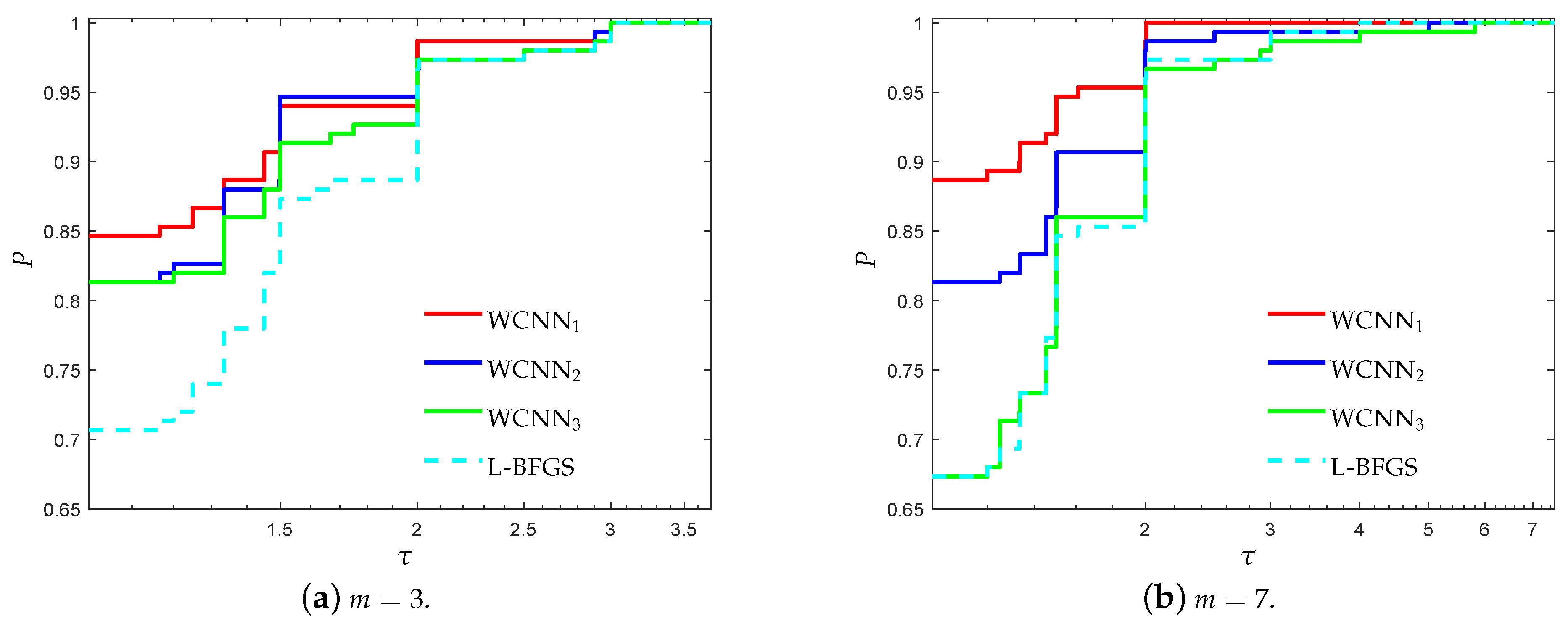
Figure 2.
Log10 scaled performance profiles based on F1-score for the breast cancer classification problem.
Figure 2.
Log10 scaled performance profiles based on F1-score for the breast cancer classification problem.
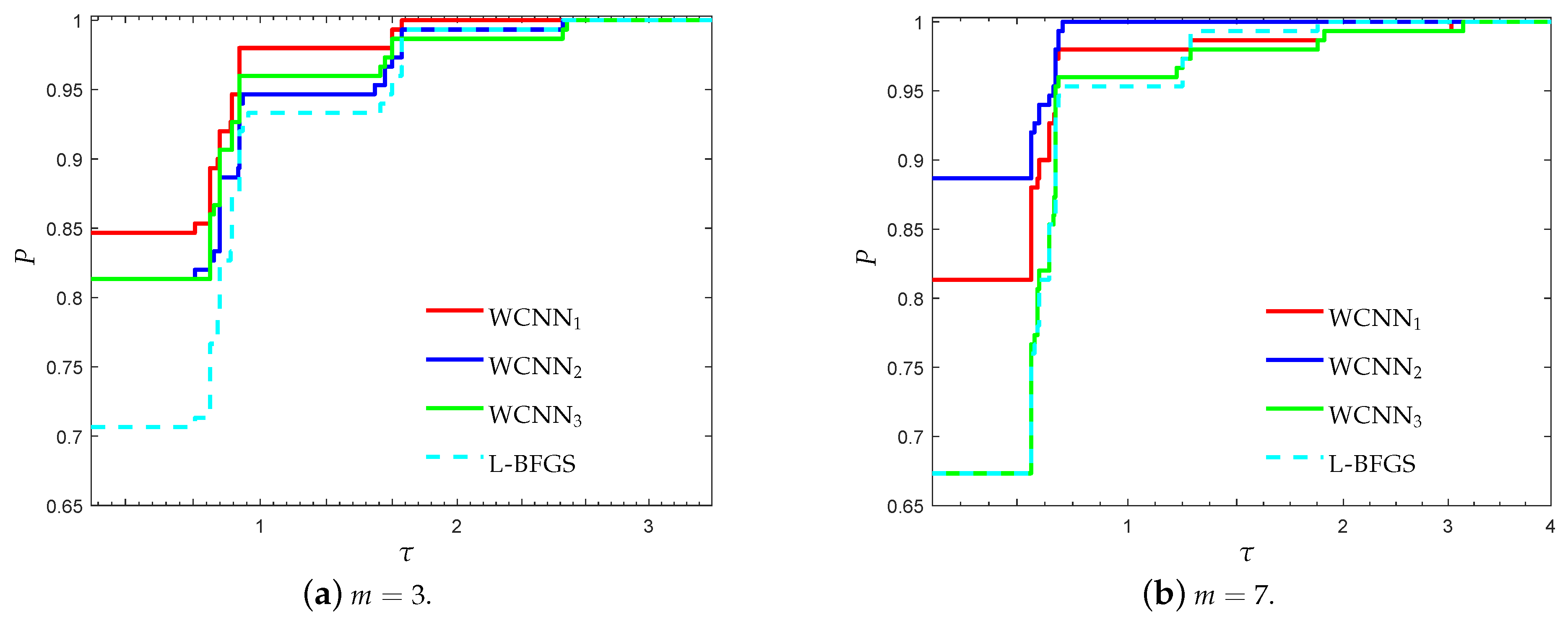
Figure 3.
Log10 scaled performance profiles based on accuracy for the Australian credit card classi-fication problem.
Figure 3.
Log10 scaled performance profiles based on accuracy for the Australian credit card classi-fication problem.

Figure 4.
Log10 scaled performance profiles based on F1-score for the Australian credit card classi-fication problem.
Figure 4.
Log10 scaled performance profiles based on F1-score for the Australian credit card classi-fication problem.

Figure 5.
Log10 scaled performance profiles based on accuracy for the diabetes classification problem.
Figure 5.
Log10 scaled performance profiles based on accuracy for the diabetes classification problem.

Figure 6.
Log10 scaled performance profiles based on F1-score for the diabetes classification problem.
Figure 6.
Log10 scaled performance profiles based on F1-score for the diabetes classification problem.

Figure 7.
Log10 scaled performance profiles based on accuracy for the Escherichia coli classification problem.
Figure 7.
Log10 scaled performance profiles based on accuracy for the Escherichia coli classification problem.

Figure 8.
Log10 scaled performance profiles based on F1-score for the Escherichia coli classification problem.
Figure 8.
Log10 scaled performance profiles based on F1-score for the Escherichia coli classification problem.

Figure 9.
Log10 scaled performance profiles based on accuracy for the Coimbra classification problem.
Figure 9.
Log10 scaled performance profiles based on accuracy for the Coimbra classification problem.

Figure 10.
Log10 scaled performance profiles based on F1-score for the Coimbra classification problem.
Figure 10.
Log10 scaled performance profiles based on F1-score for the Coimbra classification problem.
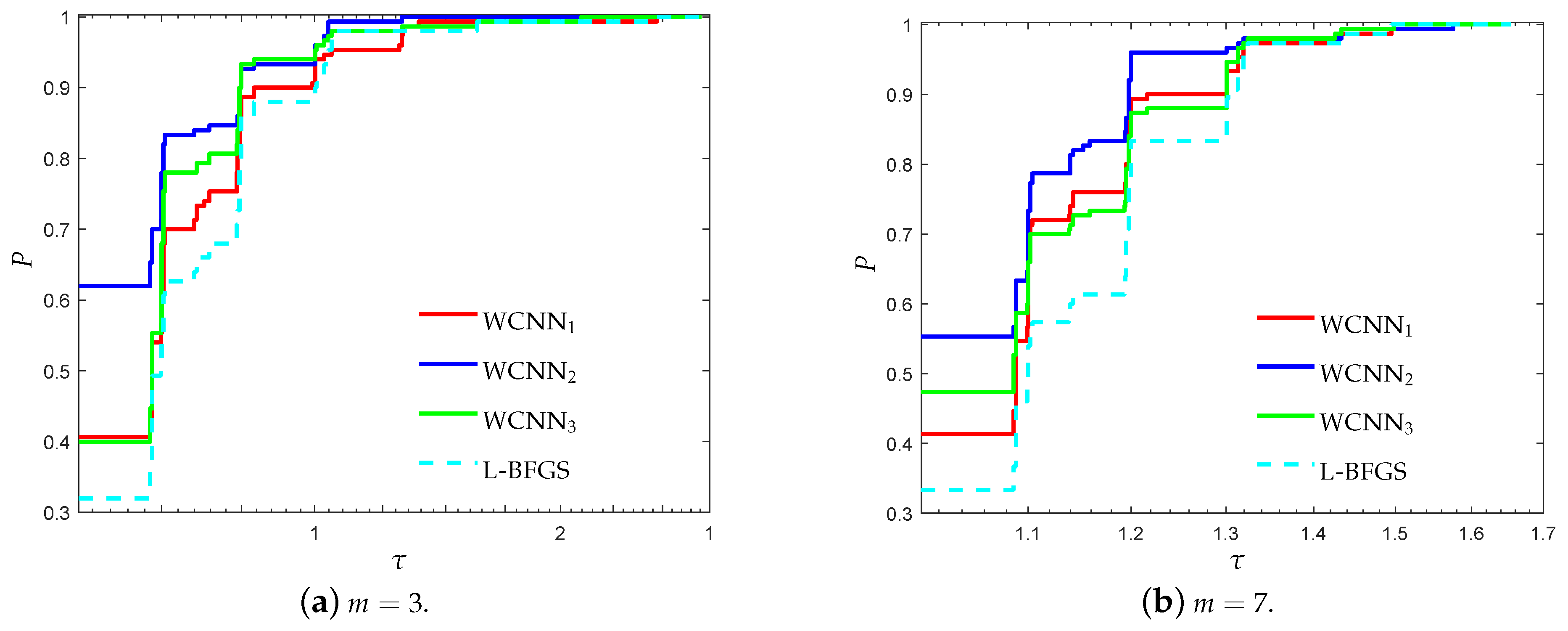
Figure 11.
Log10 scaled performance profiles based on accuracy for the SPECT heart classification problem.
Figure 11.
Log10 scaled performance profiles based on accuracy for the SPECT heart classification problem.

Figure 12.
Log10 scaled performance profiles based on F1-score for the SPECT heart classification problem.
Figure 12.
Log10 scaled performance profiles based on F1-score for the SPECT heart classification problem.

Figure 13.
Log10 scaled performance profiles based on accuracy of WCNN against the state-of-the-art training algorithms RPROP, SCG and LM.
Figure 13.
Log10 scaled performance profiles based on accuracy of WCNN against the state-of-the-art training algorithms RPROP, SCG and LM.
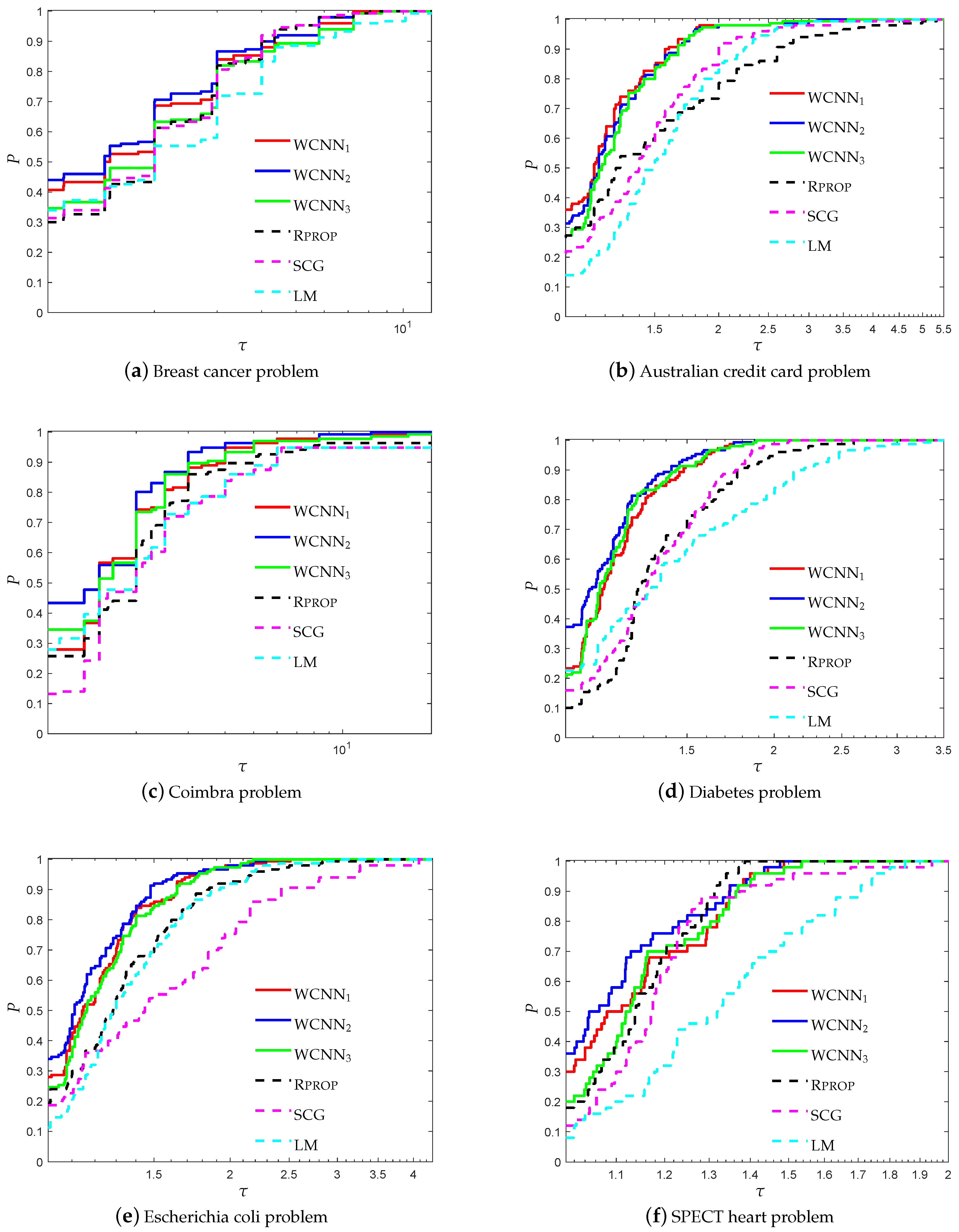
Figure 14.
Log10 scaled performance profiles based on F1-score of WCNN against the state-of-the-art training algorithms RPROP, SCG and LM.
Figure 14.
Log10 scaled performance profiles based on F1-score of WCNN against the state-of-the-art training algorithms RPROP, SCG and LM.


Table 1.
Brief description of datasets and neural network architectures used in our study.
| Classification Problem | #Features | #Instances | Neural Network Architecture | Total Number of Weights |
|---|---|---|---|---|
| Breast cancer | 9 | 683 | 9-4-2-2 | 56 |
| Australian credit card | 15 | 690 | 15-16-8-2 | 410 |
| Diabetes | 8 | 768 | 8-4-4-2 | 66 |
| Escherichia coli | 7 | 336 | 7-16-8 | 264 |
| Coimbra | 9 | 100 | 9-5-2-2 | 68 |
| SPECT heart | 13 | 270 | 13-16-8-2 | 230 |
© 2018 by the author. Licensee MDPI, Basel, Switzerland. This article is an open access article distributed under the terms and conditions of the Creative Commons Attribution (CC BY) license (http://creativecommons.org/licenses/by/4.0/).
Share and Cite
MDPI and ACS Style
Livieris, I.E. Improving the Classification Efficiency of an ANN Utilizing a New Training Methodology. Informatics 2019, 6, 1. https://doi.org/10.3390/informatics6010001
AMA Style
Livieris IE. Improving the Classification Efficiency of an ANN Utilizing a New Training Methodology. Informatics. 2019; 6(1):1. https://doi.org/10.3390/informatics6010001
Chicago/Turabian StyleLivieris, Ioannis E. 2019. "Improving the Classification Efficiency of an ANN Utilizing a New Training Methodology" Informatics 6, no. 1: 1. https://doi.org/10.3390/informatics6010001
Note that from the first issue of 2016, this journal uses article numbers instead of page numbers. See further details here.