Artery Segmentation in Ultrasound Images Based on an Evolutionary Scheme

Abstract

Segmentation in ultrasound (US) images is a challenge in computer vision, due to the high signal noise, artifacts that produce discontinuities in the boundaries and shadows that hide part of the received signal. In this paper, a solution based on ellipse fitting motivated by natural artery geometry will be proposed. To optimize the parameters that define such an ellipse, a strategy based on an evolutionary algorithm was adopted. The paper will also demonstrate that the method can be solved in a reasonable amount of time, making intensive GPGPU (general graphics processing unit, GPU, processing) where excellent computing performance gain is obtained (up to 54 times faster than the parallel CPU implementation). The proposed approach is compared with other artery segmentation methods in US images, obtaining very promising results. Furthermore, the proposed approach is parameter free and does not require any initialization estimation close to the final solution.

1. Introduction

In medical imaging, one of the most important topics, which usually turns into a complex task, is image segmentation. Diagnosis based on the measurement of the dimensions of the artery allows experts to identify diseases, such as aneurysm. This disease produces an oversizing in the artery with the risk of a possible rupture. Hence, a good segmentation of the artery based on ultrasound (US) imaging is important, as it is used for diagnosing different vascular pathologies, such as aneurysm. US imaging represents a crucial medical tool to measure any oversize of the artery given its noninvasive nature, instead of other invasive techniques that make the use of contrast agents. These other techniques are inefficient and expensive as regards their actual cost, in terms of time consumption, and regarding the need for human resources with specific skills. Though US-based explorations require highly specialized personnel, approaches, such as the one described here, aim to create a valid tool, even for not so highly specialized staff.

This paper is focused on segmenting the outer side of the artery in US imaging, in an easy way, reducing the requirement for specific training, also reducing in this way the inter-intra-specialist variability and, thus, increasing the reliability of the measurements of the diameter of the artery. Semiautomatic measurement schemes, such as the one described in this work, also aim to facilitate the US exploration process, making it suitable even for medical personnel with less specific exploration skills. Figure 1 shows an example of a manual segmentation in typical US software. At first, the artery is detected, and the frame is frozen to be analyzed. On this static image, the expert measures, by means of two perpendicular lines, the diameter of the artery. This technique becomes quite rudimentary, because it requires a certain degree of specialization, and even so, the final measurement depends on the current manual skill during the measurement estimation. This leads to high inter-intra-specialist evaluation variability.

Figure 1. Typical manually-driven measurement in ultrasound (US) software (TeleMed) to determinate the diameter of the artery.

Figure 1. Typical manually-driven measurement in ultrasound (US) software (TeleMed) to determinate the diameter of the artery.

The main contribution of this work is the proposal of a novel method based on the geometric nature of the artery, which adopts elliptical shapes. This method is able to segment the artery more accurately than other models proposed in the literature. The optimization of the seed ellipse parameters is done with an evolutionary optimization approach. Due to the high computational cost of the evolutionary models, it will make use of massive parallel architectures and present-day complex algorithms to carry out the segmentation in a reasonable time. The proposed approach is evaluated and compared with other well-known segmentation techniques, obtaining very promising results in comparison with the state-of-the-art.

Nowadays, many solutions have been proposed in natural imaging to detect ellipses. One of them is the approach proposed by Yao et al. [1], where the possibility of making use of a multi-population genetic algorithm, which turns out to be a more robust and faster solution than classic methods, such as the randomized Hough transform (RHT) [2], was demonstrated. Similar works have been carried out by Lutton and Martinez [3] or Mainzer [4]. In these works, genetic algorithms were also used to detect ellipses in natural images. This kind of method cannot be extrapolated to the US domain because of the existence of several artifacts, such as not-well-defined edges, noise and the presence of high discontinuities in the edges, etc. It is also important to remark that those approaches are only based on the binary domain and focused on natural images. In the US framework, an approach also based on ellipse estimation has been recently proposed by Moursi and Sakka [5]. This method first applies a segmentation to obtain an early approximation of the ellipse parameters and is subordinated to the pre-segmentation stage; if this stage fails, the rest of the segmentation stages will also fail.

The paper is organized as follows: Section 2 introduces a detailed explanation of the proposed method and four common segmentation techniques to evaluate the quality of the described approach; the graphics processing unit (GPU) implementation of the suggested method, the obtained performance and a comparison with a parallel CPU implementation are also detailed in this section. Section 3 compares the accuracy of the introduced method with respect to the state-of-the-art approaches, while Section 4 will discuss the obtained results of the evaluated methods. Finally, Section 5 summarizes some conclusions.

2. Materials and Methods

2.1. Evaluated Segmentation Methods

In this subsection, the most common segmentation methods in medicine will be briefly described and compared with the submitted approach.

2.1.1. Parametric Active Contour

Kass et al. [6] proposed a model that consists in parameterizing the curve based on the topology of the image and the internal features of the curve. Given a curve v(s) = [x(s),y(s)], s ∊ [0,1], the objective is to fit such a curve to the nearest contour. Hence, Equation (1) is minimized.

(1)

where F_int(v(s)) is the internal force, F_ext(v(s)) the external force, F_const(v(s)) another external force (e.g., one given by the user) and F_Balloon(v(s)) an external force that provides expansion or contraction to the contour. The internal force can be defined as in Equation (2).

(2)

The first term, F_cont, minimizes the length of the arc and α controls the elasticity of the contour. On the other hand, the second term, E_curv, minimizes the curve, and β handles the flexibility and smoothness of the contour.

The original approach [6] was prone to problems when the initialization was far away from the solution. The use of the external force F_ext (v(s)) aims to minimize this problem. As Xu and Prince [7] propose, expanding the external force field equation with a model that produces vector diffusion Equation (3) called gradient vector flow.

(3)

where µ is a non-negative weight that provides the degree of smoothness, f_x and f_y are the initial external force vectors and (u,v) the new estimated vectors. The last term is motivated by the approach of L. Cohen and I. Cohen [8], which included a new extra external force able to inflate or deflate the shape of the contour, and it is defined in Equation (4), where γ ∊ [−1,1], causing the negative values to be a deflation of the shape and the positive ones an inflation. This method has been used, for instance, to approximate the Gallbladder’s shape [9], to segment tumors in livers [10] or to segment skin cancer [11].

(4)

2.1.2. Region-Based Active Contour Model (ACM)

Zhang et al. [12] proposed a novel method that allows a selective segmentation by means of a combination of the geodesic active contour [13] and the Chan–Vese methods [14]. This model makes use of the signed pressure force (SPF), i.e., it modulates the expansion or contraction force of the region of interest, as indicated in Equation (5).

(5)

where u₀ is the original image and c1 and c2 are the means of the internal and external regions of the level set. SPF works as a constraint of the region. Hence, Zhang et al. [12] removed the weight by the SPF function in geodesic active contour Equation (6), where g(|∇I|) is the diffusivity function, ϕ the active contour, f the balloon force, which allows one to control the shrinking or expanding of the contour, and α a constant to control the diffusion on weak edges.

(6)

(7)

The Chan–Vese method has no problem with the leaks; for that reason, ∇g(|∇I|)^T·∇ϕ is removed, because it is no longer needed. Furthermore, the diffusion term in the original Equation (6) was substituted by a Gaussian convolution. Hence, the final equation after the modifications explained above is simplified as indicated in Equation (7).

2.1.3. Segmentation Based on Fuzzy C-Mean Clustering

Fuzzy C-mean (FCM) [15] has become a popular method for segmentation in medical imaging. Abdel-Dayem and El-Sakka [16] make use of this method to segment the carotid in US imaging, where the features that make up the clustering data are formed by the intensity, mean and standard deviation of a 5 × 5 block. Once the feature vector is extracted per each pixel, the FCM is used to segment the image into three classes. Finally, the user selects the desired segmented area, and by means of morphological reconstruction [17], the selected area will be extracted from the rest.

2.1.4. Active Shape Models (ASMs)

Incorporating shape prior knowledge has been one of the most recent advances in segmentation in the last decade. Cootes et al. [18] proposed a statistical method for the shape that can be deformed with respect to the mean through the most relevant eigenvectors (P) and a parameter, b, as indicated in Equation (8).

x = x + P · b

(8)

The objective of this method is to estimate the parameters to locate the desired object to be segmented by means of matching each landmark with the previously trained normalized gradient profiles and solving linear equations to estimate the desired parameters in a multi-scale strategy. Those parameters are the translation in the x- and y-axis, scale, rotation and deformation Equation (9). In this evaluation test, seven different kinds of artery topologies were trained in four scales and twelve landmarks per scale, which is enough to cover the common cases.

v = {t_x,t_y,s,θ,b}

(9)

2.2. Proposed Segmentation Method

As an alternative to the described methods to segment the artery based on US images, this work is based on the proposal of a well-known stochastic technique. Storn and Price [19] designed a method based on an evolution scheme to find optimal parameters in a subset of the solutions space, called differential evolution (DE). This method has demonstrated that working on low-dimensional problems [20], a good performance is obtained. The main objective of the proposed segmentation method is to find the parameters of a given ellipse that better fit in the boundaries of the artery. This optimization problem is addressed using DE to obtain the parameters (x_c,y_c,a,b,θ) that define ellipse Equation (10), as indicated in Figure 2.

x(t) = x_c + a ∙ cost ∙ cosθ − b ∙ sint ∙ sinθ
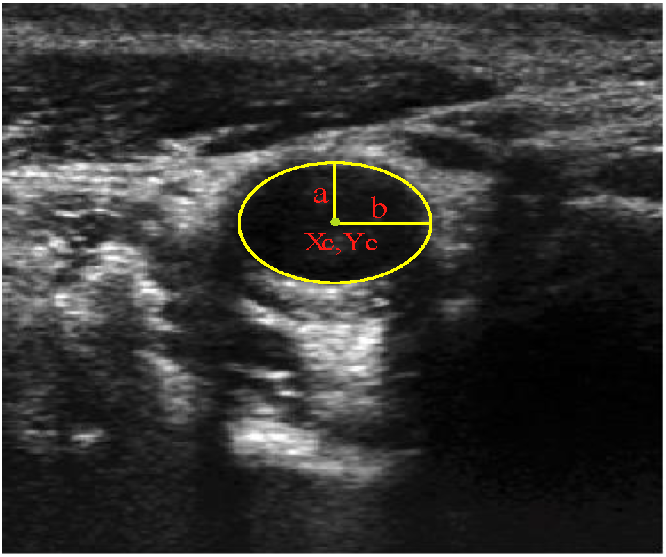
y(t) = y_c + a ∙ cost ∙ sinθ − b ∙ sint ∙ cosθ

(10)

where x_c and y_c are the center coordinates of the ellipse, a and b the minor and major axis, θ the angle with respect to the x-axis and the major axis of the ellipse and t a parameter that varies within the range [0−π].

The pseudo-code of DE is shown in Algorithm 1, where the InitPopulation is a function that initializes the population in a bounded space defined by the maximum and minimum values of the parameters (MaxPar and MinPar). The fitness function (GetFitness) defines how well the parameters of the agents fit with the desired function (see Section 2.2.2 for more information about the fitness function). To provide an exploration option to the population in each generation, a mutation operator (Mutate) is included. The new mutated agent is defined in Equation (11); where agents of the same generation ( ) are used to estimate the new one, with a desired mutation factor (F). Different approaches of this operator will be evaluated in Section 3. Another important exploration mechanism is the one provided by the cross-operator (Cross), where the mutated agents will be mixed with the current generation with a probability factor, CR (Cross Rate).

(11)

Figure 2. Illustration fitted in the boundaries of an artery.

Figure 2. Illustration fitted in the boundaries of an artery.

Algorithm 1. Differential evolution (DE) pseudocode implementation.

• 1 Population = InitPopulation(MaxPar,MinPar);
• 2 FitPop = GetFitness(Population);
• 3 BestAgent = GetBestAgent(Population);
• 4 while (NumIter < NumIterMax)
• 5 MutPop = Mutate(Population,BestAgent,F);
• 6 CrPop = Cross(Population,MutPop,CR);
• 7 FitCr = GetFitness(CrPop);
• 8 Population = Replace(Population,CRPop,FitCr,FitPop);
• 9 BestAgent = GetBestAgent(Population);
• 10 NumIter = NumIter + 1;
• 11 end while
• 12 return BestAgent

At this point, the main parameter optimization method used in this paper has been defined. The next subsection will detail the features extracted in the US image used by the DE model to find the desired ellipse parameters that define the best contour of the artery. This search will be led by an ad hoc multi-objective function, as explained in Subsection 2.2.2, to solve this problem.

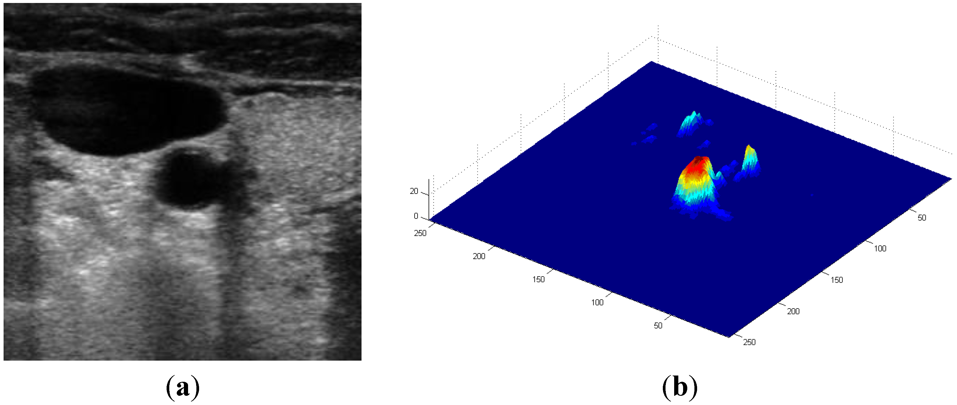
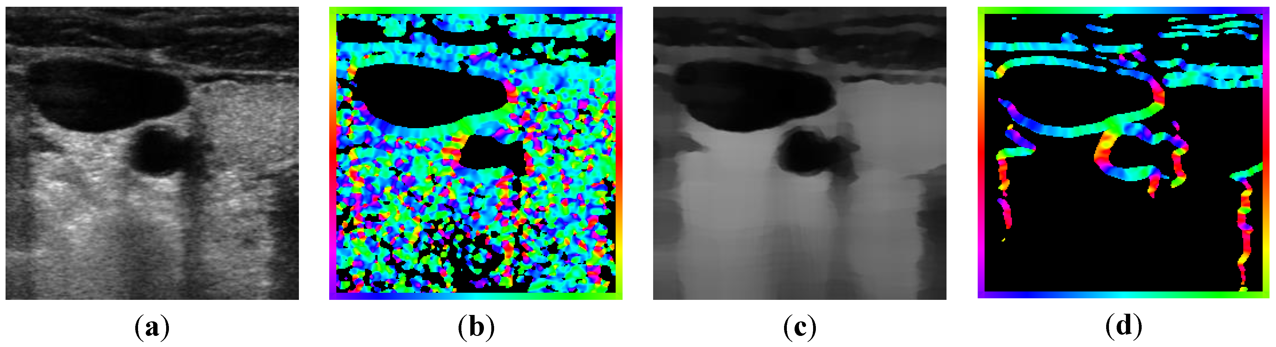
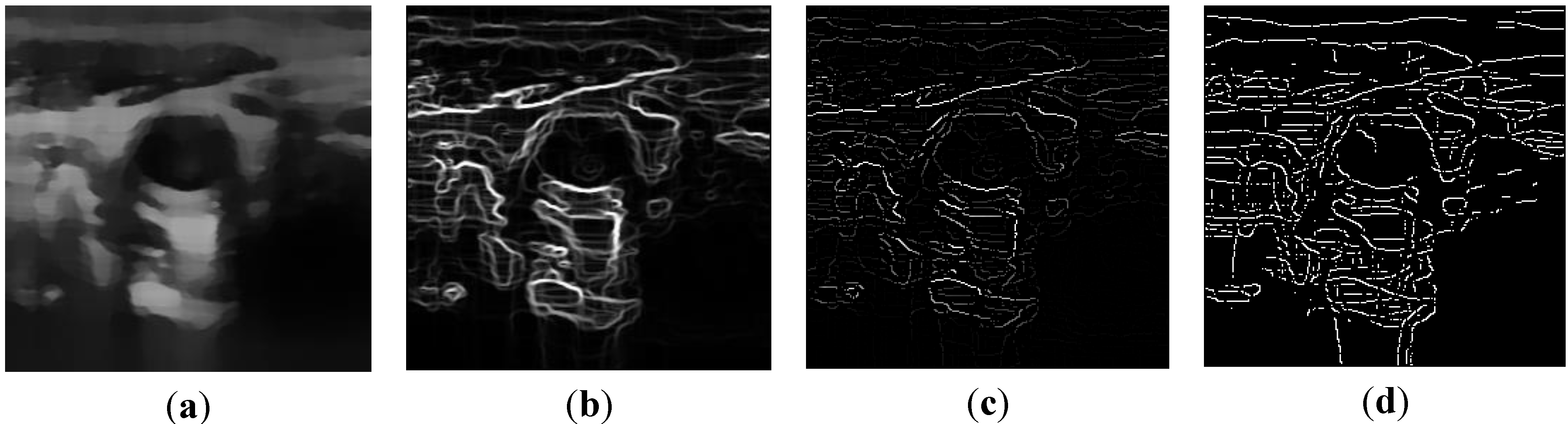
2.2.1. Feature Extraction

To address the DE method over the solution space and estimate the parameters that obtain the best ellipse fitting over the artery, it is necessary to extract features that make it easier to find the desired solution. At first, the proposed approach must estimate the potential x_c and y_c parameters, which define the center of the ellipse by means of the method proposed by Loy and Zelinsky [21], known as fast radial symmetry (FRS). This algorithm is based on a voting system, which determines the positive and negative affected pixels, p_+ve, through the norm of the gradient, 𝑔(p), at point p using a ratio of size n, the orientation projection image, , and the magnitude projection image, .

(12)

(13)

(14)

To determinate the saliency map,S, Equation (16), the result of Equation (15) is convolved with a Gaussian to remove any undesired noise. Parameter α in Equation (15) acts as a gain factor of the saliency map to allow the enhancement of low contrast voting gradients.

F_n(p) = ||O_n(p)||^(α)M_n(p)

(15)

(16)

As opposed in the original version of this method, the normalization of Equations (13) and (14) and the integration of S Equation (16) are not performed. These changes are done so as to obtain a faster implementation, as explained in Subsection 2.3. Figure 3b shows an example of the output obtained after applying the FRS algorithm to an US image.

At this point, one of the functions that will drive the DE method to optimize parameters x_c and y_c has been described. The guidance functions to obtain a, b and θ parameters in expression Equation (10) will be based on edge features, in this case, on the pixel orientation, gradient and binarized edges. The pixel orientation is estimated by means of the eigenvector with a high eigenvalue of the first order structure tensor J Equation (17), where I_x, I_y and I_xy denote the spatial derivates and G_σ a Gaussian convolution for each spatial derivate.

(17)

Figure 3. (a) Original image and (b) saliency map after applying fast radial symmetry.

Figure 3. (a) Original image and (b) saliency map after applying fast radial symmetry.

One of the main problems of working with US images is the amount of speckle noise. Yongjian and Acton [22] described a solution to reduce the speckle noise, named Speckle Reducing Anisotropic Diffusion (SRAD), where a non-linear diffusion method to estimate the strength of the edges in US images through instantaneous coefficient of variation (ICOV) Equation (18) is suggested. To obtain the degree of exchange in the diffusion scheme, Yongjian and Acton use mechanism Equation (19), where the diffusion becomes zero in areas with highly contrasted edges and the opposite case when the area is flat. Parameter determinates the level of speckle noise, and therefore, it allows the control of the diffusion over time in Image (I).

(18)

(19)

Such noise will interfere in the pixel orientation estimation, as shown in Figure 4b. To avoid this artifact, the SRAD method will be applied with the objective of removing the noise and the texture generated by the tissue to obtain a clear pixel orientation, as illustrated in Figure 4d.

Figure 4. (a) Original US image; (b) pixel orientation of the original image; (c) SRAD smoothing; (d) pixel orientation of the smoothed (SRAD) image. In b and c, the pixel local orientation is represented with colors with respect to the color reference frame.

Figure 4. (a) Original US image; (b) pixel orientation of the original image; (c) SRAD smoothing; (d) pixel orientation of the smoothed (SRAD) image. In b and c, the pixel local orientation is represented with colors with respect to the color reference frame.

Figure 5. (a) US image smoothed with SRAD; (b) LIP-Sobel gradient; (c) non-max suppression applied to LIP-Sobel gradient estimation; (d) binary representation of the edges.

Figure 5. (a) US image smoothed with SRAD; (b) LIP-Sobel gradient; (c) non-max suppression applied to LIP-Sobel gradient estimation; (d) binary representation of the edges.

However, this information is not enough yet to address the search. Given the large solution space provided by the pixel orientation, edge information will be incorporated to define the echogenicity. A change of different tissue structures, such as muscle to fat or artery layers to blood, provides a high degree of echogenicity. For this reason, the Logarithmic Image Processing (LIP) edge detector [23] is used. This detector makes use of the logarithm derivatives [24] with the objective of enhancing such areas as much as possible. Figure 5a shows the US image filtered by the SRAD method, while Figure 5b illustrates the obtained result after applying the LIP-Sobel gradient. The non-max suppression [25] results are shown in Figure 5c and finally; the binary map (Figure 5d) after thresholding the non-max suppression output is included.

2.2.2. Ellipse Parameter Estimation

Once the features that will drive the evolutive method to obtain the parameters (x_c, y_c,a,b,θ) that define ellipse Equation (10) have been defined, the fitness function of the DE algorithm will be described in this section. The proposed method intends to minimize the angle difference between the norm vectors of the ellipse and the pixel orientation of the image and, at the same time, to maximize the gradient and the binary edge of the artery and maximize the centricity through FRS. To solve this problem, the method proposed by Hajela and Lin [26] is adopted, where the approach follows a strategy based on weights for each different objective to integrate them into a unique fitness function. The proposed implementation makes use of a penalty scheme that penalizes points of the ellipse where clear orientation, gradient or edge Equations (21)–(23) do not exist. This penalization will be adaptive, by means of Equation (20), where the degree of penalization is defined by the Euclidean norm of the axis of the ellipse and its ratio aspect. A weight factor will be also included to this penalization. After an empirical evaluation, it was demonstrated that by setting those values to W_o = −90, W_𝑔 = −1 and W_b = −1, the method obtains reasonable results.

(20)

(21)

(22)

(23)

f_FRS(x_c,y_c) = FRS(x_c,y_c)

(24)

The first objective function Equation (21) is the orientation error, f_o, which estimates the generated angle between the norms of the ellipse vector, ( ), and the pixel orientation, ( ), vector by means of function A_v, which defines the angle between both vectors. The second objective function, f_𝑔, Equation (22), aims to find shapes with a higher echogenicity given by the LIP-Sobel gra2-dient, G_v. To avoid the gradient generated by small variations in the intensity of the image, a threshold scheme is utilized. The function is set to the gradient if the threshold is higher than a defined value; otherwise, a penalization is applied to avoid the discontinuity in the shape of the ellipse and the gradient map. The third objective function, f_b, Equation (23), acts in a similar way as the previous one, but in this case, a binary map, B_v, is used. Finally, the fourth objective function, f_FRS, Equation (24), will guide the ellipse into the center of the artery using the FRS map. Once all the objective functions have been defined, the fitness function can be expressed as shown in Equation (25), where the weights, α₁,α₂,α₃,α₄, are incorporated for each respective objective function. After empirical tests, it was found that those values fixed to α₁ = 100, α₂ = 2, α₃ = 100, α₄ = 30 of the proposed method achieve satisfactory results.

(25)

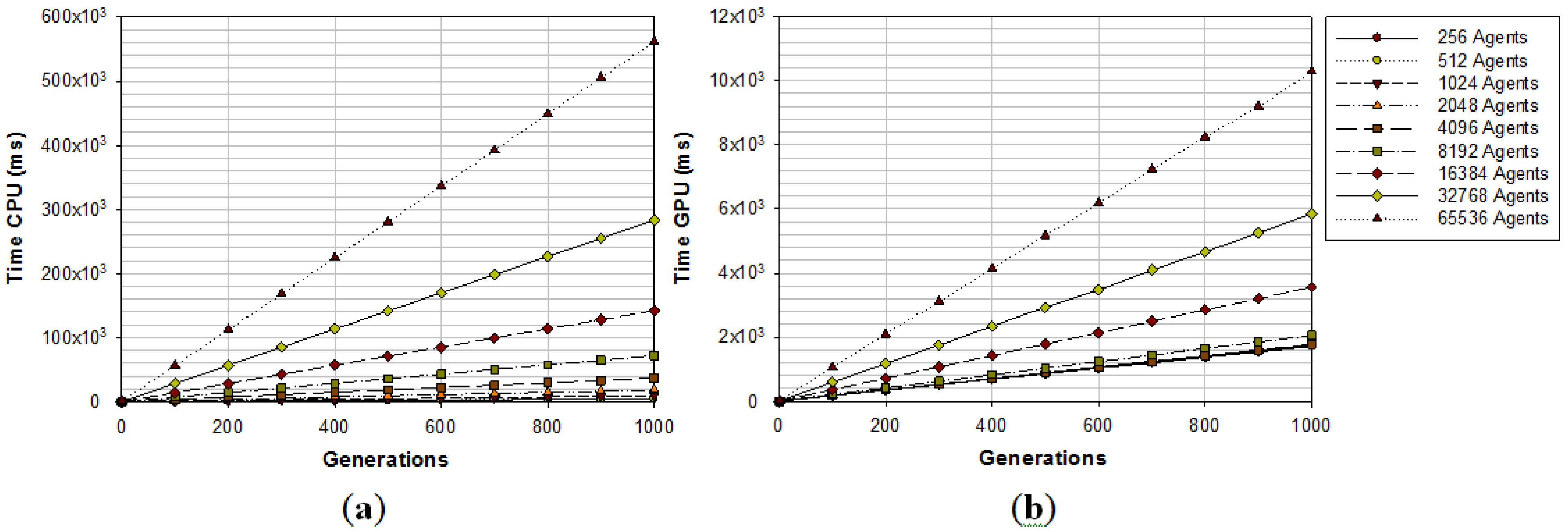
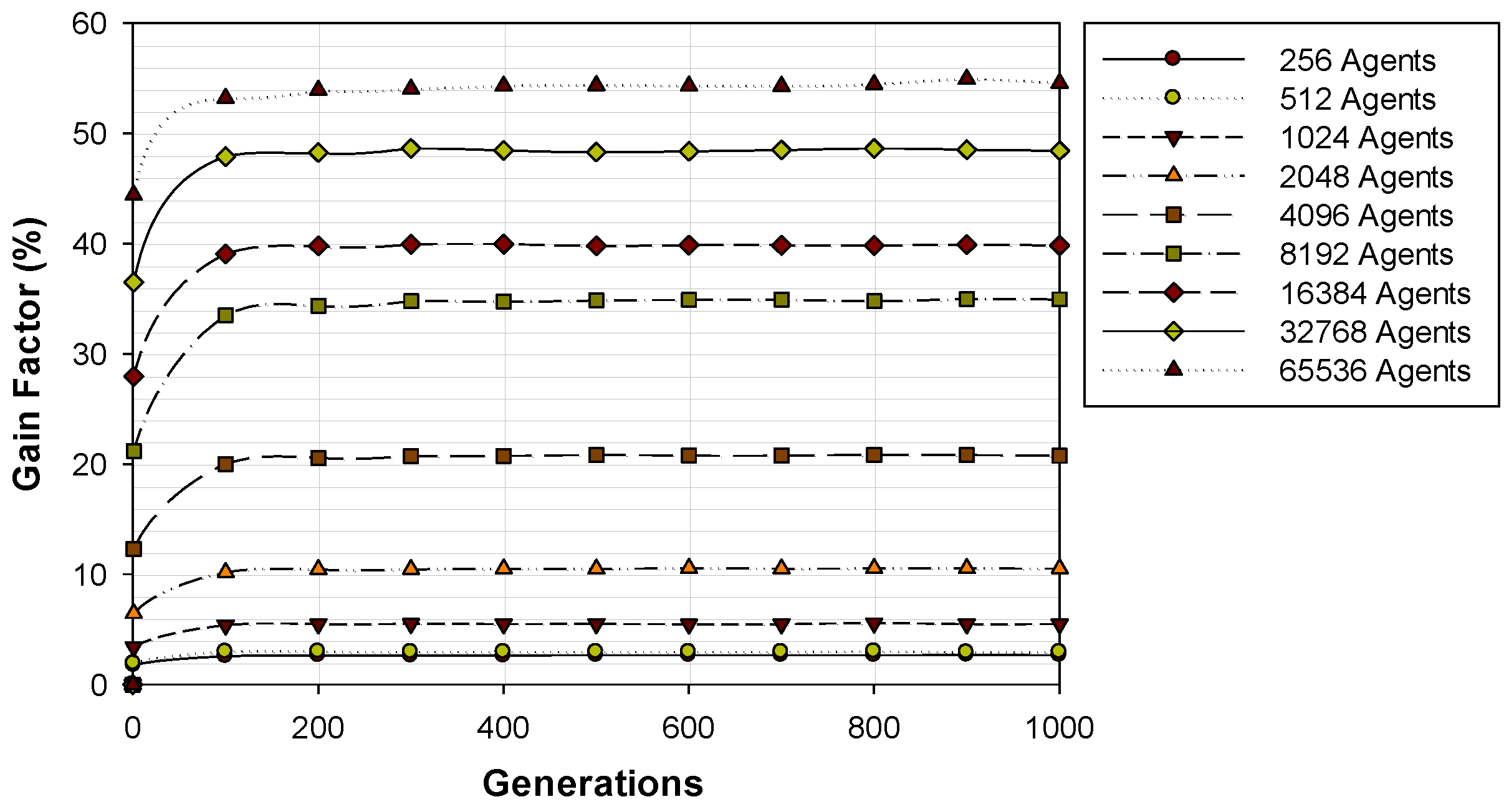
2.3. GPU Implementation

One of the main problems when making use of evolutive schemes is the computation cost, because it requires many iterations (generations) and a considerable number of individual members in each population. To avoid this limitation, a well-known parallel computing architecture, GPU (graphics processing unit), is utilized. The GPU used to evaluate the proposed implementation is NVidia GTX 580 (Fermi architecture; NVidia Corporation, Santa Clara, Calif., US), and it is equipped with 512 processing cores. In this section, the same implementation is also compared with an Intel i7 CPU 950 (Intel Corporation, Santa Clara, Calif., US) that incorporates eight cores (four cores with two logic-cores per each physical one). The technology used to develop the methods, in both architectures, is Open Computing Language (OpenCL), motivated by its degree of versatility to be executed in different platforms. At this point, the implementation will be briefly described and the differences with other proposed methods in literature will be listed.

The differential evolution method has a 100% parallel nature and is very suitable for parallel architectures, such as GPUs [27,28,29], The adopted scheme is similar to the one described in [27], with the difference being that the XorShift pseudorandom number generator [30] is used instead of generating random vectors in the host in each generation, with the objective of speeding up the performance. In the evaluation of the proposed method, it is important to remark that unlike other approaches; the advantage of the parallelism on a CPU was taken into account (making use of all cores in parallel) to evaluate, in the most equitable way, the performance of both architectures (GPU and CPU). It has been demonstrated [31] that the number of agents (the size of the DE population of solutions) matters; a small number of agents can produce an early convergence. Therefore, an assessment is carried out by taking into consideration the number of agents compared to the number of generations. Figure 6 shows the performance evaluation considering the number of agents and number of generations in the CPU (Figure 6a) and GPU (Figure 6b). In Figure 7, the gain factor obtained on the GPU with respect to the CPU is illustrated, and it shows a significant gain in performance (up to 54 times faster). After some experimental tests, it was noticed that the use of 4,096 agents and 200 generations is enough to ensure the convergence to an optimized solution.

Figure 6. Time consumption of the differential evolution algorithm in a (a) parallel CPU and (b) a GPU implementation.

Figure 6. Time consumption of the differential evolution algorithm in a (a) parallel CPU and (b) a GPU implementation.

Figure 7. The factor obtained on the GPU with respect to the parallel CPU implementation.

Figure 7. The factor obtained on the GPU with respect to the parallel CPU implementation.

Once DE is evaluated in terms of computational speed on a GPU and parallel CPU, the feature extraction implementation in the US images (256 × 256) on the GPU is detailed. The parallel implementation of the SRAD and FRS methods will be explained in more detail, but the rest of the methods will not be described here, because their implementation is trivial and does not represent any kind of novelty. Nevertheless, all the performance rates of the specific modules are benchmarked in Table 1.

SRAD, as well as non-lineal diffusion methods in general, is very expensive in computation terms. Weickert [32,33] proposed a semi-implicit scheme to speed up this kind of method: denominated additive operator splitting (AOS). In a recent work, Cao et al. [34] exposed a SRAD GPU implementation based on an AOS scheme. To solve the tridiagonal matrix system, which is involved in the AOS method, Cao et al. utilized the cyclic reduction (CR) [35] method. In this work, the parallel cyclic reduction (PCR) [36] technique was chosen, due to the fact that it has an impact on the processing gain factor [37] in comparison with CR. This approach is a mix of processing techniques, where each system is executed in parallel, and the elements of the system are solved into an iterative parallel scheme.

Table 1. Computation time evaluation of the main methods used in the proposed algorithm on the graphics processing unit (GPU) and parallel CPU implementation. AOS, additive operator splitting; FRS, fast radial symmetry.

Method	GPU Time	CPU (8 cores) Time
SRAD (AOS)5 Iterations	7.65 ms	13.58 ms
FRS	3.78 ms	-
Pixel Orientation	1.14 ms	6.95 ms
Non-Max Suppression	0.16 ms	2.29 ms
LIP-Sobel Gradient	0.11 ms	1.42 ms

Table 1. Computation time evaluation of the main methods used in the proposed algorithm on the graphics processing unit (GPU) and parallel CPU implementation. AOS, additive operator splitting; FRS, fast radial symmetry.

Method	GPU Time	CPU (8 cores) Time
SRAD (AOS)5 Iterations	7.65 ms	13.58 ms
FRS	3.78 ms	-
Pixel Orientation	1.14 ms	6.95 ms
Non-Max Suppression	0.16 ms	2.29 ms
LIP-Sobel Gradient	0.11 ms	1.42 ms

On the other hand, the FRS algorithm presents a sequential processing that becomes quite difficult to parallelize on a GPU. To solve this problem, Glavtchev et al. [38] proposed a smart solution whose computation time becomes invariant to voting size ratio Equation (12). To solve the voting integration bottleneck, Glavtchev et al. delegated this task to Open Graphics Library (OpenGL) by means of 3D primitives. Since this solution is totally focused on being solved on a GPU, the equivalent CPU implementation cannot be performed. Regarding the LIP-Sobel method and post-processing stages (close to the LIP-Canny model), the developed approach was done in a similar way as in the work presented by Palomar et al. [39], but in the last stage, only applying non-max suppression [25] and omitting the hysteresis stage.

Finally, to conclude this section, the global time consumption is estimated. Choosing a population of 4,096 agents and 200 generations in the evolutionary scheme and the image processing analysis (detailed in Section 2.2.1), the whole computation time takes 300 ms per image. It is important to remark that in this processing time, the image transferences to the GPU and other minor algorithms, such as casting, range change, non-max suppression, thresholding, etc., are also included.

3. Results

In this evaluation, the US images were acquired from two different US devices with the objective of evaluating the methods in a non-constrained platform. Those devices are a Siemens Antares (128 lines; Siemens AG, Munich, Germany) and a TeleMed Echo Blaster (64 lines; Telemed UAB, Vilnius, Lithuania). One of the most significant differences between these pieces of US equipment is their resolution (double resolution in Siemens with respect to the TeleMed device). To determine the accuracy of the methods, the well-known F-measure estimator Equations (26)–(28) are used. This estimator evaluates a benchmark dataset of 40 US images of different patients and areas, with their respective ground truth (where an expert marked it manually, point by point).

(23)

(24)

(25)

The stochastic method differential evolution was described in Section 2.2, which states that the mutation operator aids the model to explore the space solution through Equation (11). To determine the most appropriate strategy mutation, different mutation models Equations (29)–(32) with the exposed metrics Equations (26)–(28) are evaluated.

(1)

DE/Best/1

(29)

(2)

DE/Current to Best/1

(30)

(3)

DE/Current to Best/2

(31)

(4)

DE/Rand/1

(32)

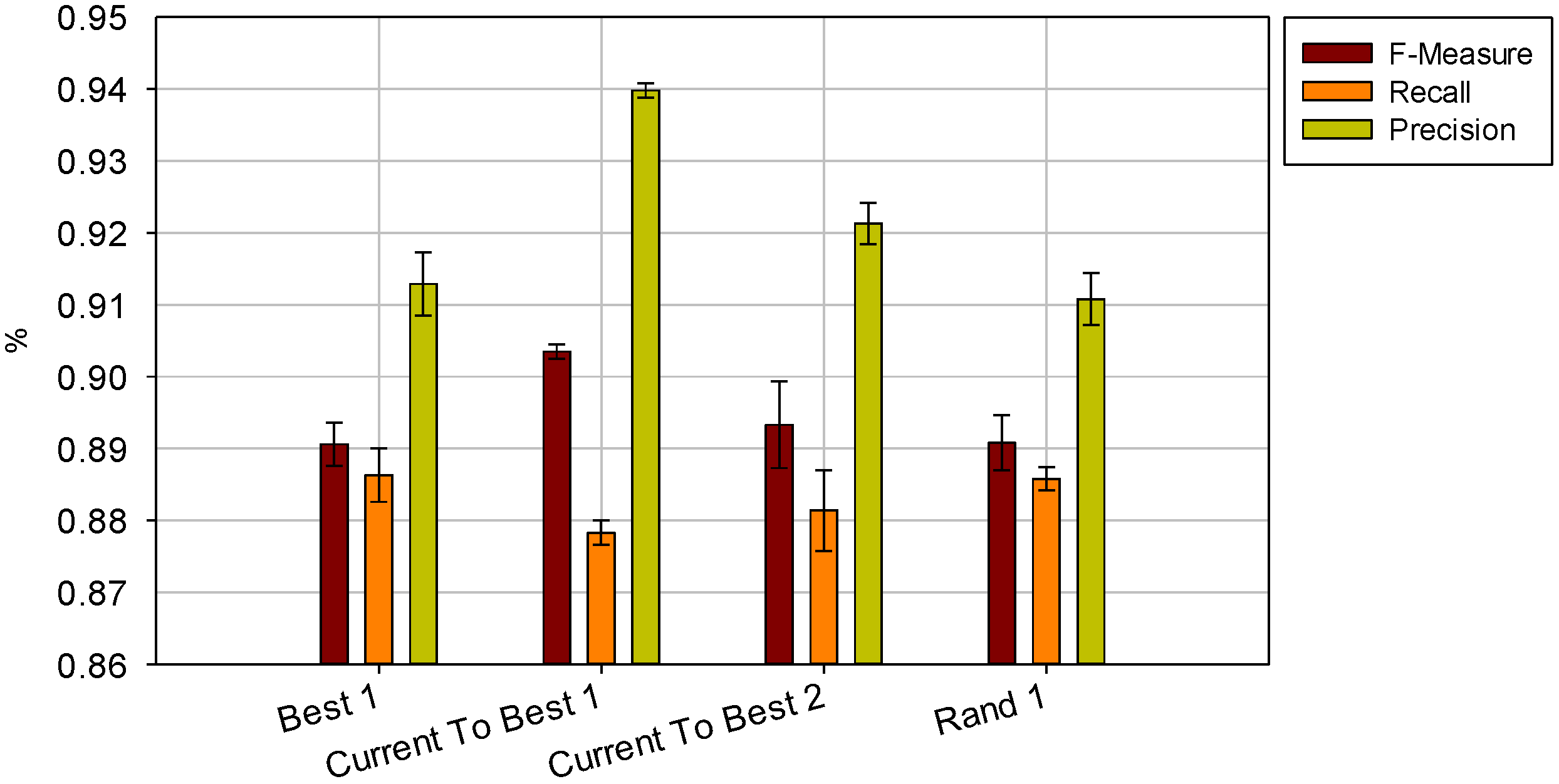
where , denotes the mutated vector, the best agent in the current generation, the current agent and and the random vectors in the evaluated generation. Figure 8 shows the obtained segmentation results with different mutation operators. To perform this test, the experiment has been repeated 10 times (per each operator) and the mean of the obtained results has been computed. It can be observed that the best mutation operation can have an impact of about 3% in precision and almost 1% in the F-measure with respect to the worst case.

Figure 8. The evaluation of the proposed method with different mutation schemes with respect to the ground truth (manually marked) with its respective standard deviations (after 10 trials in each set up).

Figure 8. The evaluation of the proposed method with different mutation schemes with respect to the ground truth (manually marked) with its respective standard deviations (after 10 trials in each set up).

It is clearly demonstrated (Figure 8) that the scheme Current to Best 1 Equation (30) is the best option, providing also a small standard deviation, while Rand 1 and Current to Best 2 schemes provide the worst results. To validate the proposed extracted features and to quantify the repercussion of each one, the impact of the combination of the features of each image is evaluated (Figure 9). It can be observed that the use of the binary mask and the edge information is not enough to find the desired parameters. The orientation feature improves the accuracy of the method up to 30% more than making use of the other features. This means that it becomes the most important characteristic in the proposed method. The rest of the features aid in refining the accuracy of the model and reduce the standard deviation in the results.

Figure 9. Evaluation of the proposed method with different features mixed (left) without orientation and (right) including the orientation feature.

Figure 9. Evaluation of the proposed method with different features mixed (left) without orientation and (right) including the orientation feature.

Figure 10. The final comparative results of the F-measure, recall and precision with respect to other state-of-the-art methods. ASM, active shape model.

Figure 10. The final comparative results of the F-measure, recall and precision with respect to other state-of-the-art methods. ASM, active shape model.

Finally, a last evaluation is carried out, where the results of the alternative methods (Section 2.1) and the proposed approach (Section 2.2) are compared. Figure 10 reveals that the presented method obtains the best results, and not only in the F-measure metric, but also in the recall and precision. In the Discussion Section, some examples of the results of this comparative evaluation are shown. Furthermore, the suggested method has an improvement in the F-measure of 3%, 5% in recall and 2% in precision with respect to active shape models (ASMs). In the case of the comparison with respect to the parametric snake method, the obtained improvement is about 4% in the F-measure, 7% in recall and 2% in precision.

To obtain a more detailed evaluation between the proposed method and the second best in the ranking, both methods are compared by means of a Bland–Altman plot. Figure 11 shows the difference between the proposed method and the second best results (ASM) and their averages. The middle line indicates the average difference of both methods, whereas the upper and lower lines represent the 95% limits of agreement with the 16.97% with respect to the mean difference. It can be concluded that Figure 11 shows an overall good agreement of the amplitudes between the presented method and the reference one (ASM).

Figure 11. The Bland–Altman figure comparing the best two obtained results (the proposed one and ASM).

Figure 11. The Bland–Altman figure comparing the best two obtained results (the proposed one and ASM).

4. Discussion

After the evaluation performed in the previous section, some results obtained with the assessed segmentation methods are exhibited, and the pros and cons of each model are discussed. Figure 12a,b shows the ground truth (red color) that defines the area of the artery. The other one, Figure 12c–l, illustrates the results obtained by the different methods, where the green color illustrates the false positives, the false negatives are marked in blue color and cyan indicates the correct segmentation. Fuzzy C-mean (Figure 12c,d) and ACM (Figure 12e,f) produce leaks in the segmentation, because these methods are not appropriate when the US image produces shadows (a quite common artifact). On the other hand, methods that preserve the shape (parametric snake, ASM and the proposed one) are more robust for handling the leaks, as is illustrated in Figure 12g,l, where such an artifact is not produced.

Figure 12. (a,b) Original US images with the ground truth marked in red; (c,d) fuzzy C-mean; (e,f) active contour model; (g,h) parametric snake; (i,j) active shape model; (k,l) proposed method. Please see the main text for the meaning of each color.

Figure 12. (a,b) Original US images with the ground truth marked in red; (c,d) fuzzy C-mean; (e,f) active contour model; (g,h) parametric snake; (i,j) active shape model; (k,l) proposed method. Please see the main text for the meaning of each color.

Comparing the group of methods that preserve the shape, it is important to remark that the parametric snake model provides different results in relation with its parameter settings (thus, it is sensitive to its internal configuration parameters). Another inconvenience occurs in the initialization of the method, which must be done close to the final solution. Those problems vanish with the ASM method, where the variation of the shape is defined in the training stage (avoiding parameter sensitivity), and its space search is longer than parametric snake, through its multiscale scheme. The suggested method does not require the training stage (unlike ASM), because it is based on the geometric nature of the artery, the ellipse.

As demonstrated in Section 3, the proposed approach reaches a good accuracy (obtaining an improvement with respect to ASM of 16.97%, as shown in the Bland–Altman figure (Figure 11), and obtains an excellent GPU performance (up to 54 times faster than the parallel CPU implementation), as demonstrated in Section 2.3. Finally, to conclude the discussion chapter, some accomplished results with the proposed method in different patients and topologies of the artery are illustrated (Figure 13).

Figure 13. Some results obtained with the proposed method in different patients.

Figure 13. Some results obtained with the proposed method in different patients.

5. Conclusions

In this work, a method based on an evolutionary approach for optimizing different kinds of features to fit an ellipse that best defines the edges of the artery has been proposed. It has been demonstrated that it can be computed efficiently making intensive use of a GPU platform. Its high accuracy in relation with other state-of-the-art methods is also highlighted.

The submitted approach outperforms other methods, not only in terms of accuracy, but also because in comparison with the ASM method, the suggested method does not require any kind of previous training stage. Another advantage that must be remarked upon is that the proposed method supports large search spaces, unlike ASM or parametric snakes, which need to be initialized close to the final solution.

In future research, we will extrapolate this approach to generalize the type of object to be segmented and will not be limited to geometric shapes.

References

- Yao, J.; Kharma, N.; Grogono, P. A multi-population genetic algorithm for robust and fast ellipse detection. Pattern Anal. Appl. 2005, 8, 149–162. [Google Scholar] [CrossRef]
- McLaughlin, R.A. Randomized Hough transform: Improved ellipse detection with comparison. Pattern Recogn. Lett. 1998, 19, 299–305. [Google Scholar] [CrossRef]
- Lutton, E.; Martinez, P. A Genetic Algorithm for the Detection of 2D Geometric Primitives in Images. In Proceedings of the 12th International Conference on Pattern Recognition, Jerusalem, Israel, 9–13 October 1994; pp. 526–528.
- Mainzer, T. Genetic Algorithm for Shape Detection. Technical Report No. DCSE/TR-2002-06. University of West Bohemia: Pilsen, Czech Republic, 2002. [Google Scholar]
- Moursi, S.G.; Sakka, M.R.E. Semi-automatic snake based segmentation of carotid artery ultrasound images. Commun. Arab Comput. Soc. (ACS) 2009, 2, 1–32. [Google Scholar]
- Kass, M.; Witkin, A.; Terzopoulos, D. Snakes: Active contour models. Int. J. Comput. Vis. 1987, 1, 321–331. [Google Scholar]
- Xu, C.; Prince, J.L. Snakes, shapes, and gradient vector flow. IEEE T. Image Process. 1998, 7, 359–369. [Google Scholar] [CrossRef]
- Cohen, L.D.; Cohen, I. Finite-element methods for active contour models and balloons for 2-D and 3-D images. IEEE T. Pattern Anal. 1993, 15, 1131–1147. [Google Scholar] [CrossRef]
- Ciecholewski, M. Gallbladder Boundary Segmentation from Ultrasound Images Using Active Contour Model. In Intelligent Data Engineering and Automated Learning–IDEAL; Springer: Berlin/Heidelberg, Germany, 2010; pp. 63–69. [Google Scholar]
- Cvancarova, M.; Albregtsen, F.; Brabrand, K.; Samset, E. Segmentation of Ultrasound Images of Liver Tumors Applying Snake Algorithms and GVF. In Proceedings of the 19th International Congress and Exhibition: Computer Assisted Radiology and Surgery (CARS 2005), Berlin, Germany, 22–25 June 2005; pp. 218–223.
- Tang, J. A multi-direction GVF snake for the segmentation of skin cancer images. Pattern Recogn. 2009, 42, 1172–1179. [Google Scholar] [CrossRef]
- Zhang, K.; Zhang, L.; Song, H.; Zhou, W. Active contours with selective local or global segmentation: A new formulation and level set method. Image Vis. Comput. 2010, 28, 668–676. [Google Scholar] [CrossRef]
- Caselles, V.; Kimmel, R.; Sapiro, G. Geodesic active contours. Int. J. Comput. Vis. 1997, 22, 61–79. [Google Scholar] [CrossRef]
- Chan, T.F.; Vese, L.A. Active contours without edges. IEEE T. Image Process. 2001, 10, 266–277. [Google Scholar] [CrossRef]
- Dunn, J.C. A fuzzy relative of the isodata process and its use in detecting compact well-separated clusters. J. Cybernet. 1973, 3, 32–57. [Google Scholar] [CrossRef]
- Abdel-Dayem, A.; El-Sakka, M. Fuzzy c-Means Clustering for Segmenting Carotid Artery Ultrasound Images. In Proceedings of the International Conference on Image Analysis and Recognition (ICIAR 2007), Montreal, Canada, 22–24 August 2007; pp. 933–948.
- Vincent, L. Morphological grayscale reconstruction in image analysis: Applications and efficient algorithms. IEEE T. Image Process. 1993, 2, 176–201. [Google Scholar] [CrossRef]
- Cootes, T.F.; Taylor, C.J.; Cooper, D.H.; Graham, J. Active shape models—Their training and application. Comput. Vis. Image Underst. 1995, 61, 38–59. [Google Scholar] [CrossRef]
- Storn, R.; Price, K. Differential evolution—A simple and efficient heuristic for global optimization over continuous spaces. J. Glob. Optim. 1997, 11, 341–359. [Google Scholar] [CrossRef]
- Hansen, N. Compilation of results on the 2005 CEC benchmark function set. Tech. Rep. Institute of Computational Science ETH Zurich. 2006. [Google Scholar]
- Loy, G.; Zelinsky, A. Fast radial symmetry for detecting points of interest. IEEE T. Pattern Anal. 2003, 25, 959–973. [Google Scholar] [CrossRef]
- Yongjian, Y.; Acton, S.T. Speckle reducing anisotropic diffusion. IEEE T. Image Process. 2002, 11, 1260–1270. [Google Scholar] [CrossRef]
- Palomares, J.M.; Gonzalez, J.; Ros, E.; Prieto, A. General logarithmic image processing. IEEE T. Image Process. 2006, 15, 3602–3608. [Google Scholar] [CrossRef]
- Deng, G.; Cahill, L.W.; Tobin, G.R. The study of logarithmic image processing model and its application to image enhancement. IEEE T. Image Process. 1995, 506–512. [Google Scholar] [CrossRef]
- Canny, J.F. A computational approach to edge detection. IEEE T. Pattern Anal. 1986, 8, 679–698. [Google Scholar] [CrossRef]
- Hajela, P.; Lin, C.Y. Genetic search strategies in multicriterion optimal design. Struct. Optim. 1992, 4, 99–107. [Google Scholar] [CrossRef]
- De Veronses, L.; Krohling, R. Differential Evolution Algorithm on the GPU with C-CUDA. In Proceedings of the IEEE Congress on Evolutionary Computation (CEC), Barcelona, Spain, 18–23 July 2010; pp. 1–7.
- Zhu, W. Massively parallel differential evolution-pattern search optimization with graphics hardware acceleration: An investigation on bound constrained optimization problems. J. Glob. Optim. 2011, 50, 417–437. [Google Scholar] [CrossRef]
- Zhu, W.; Li, Y. GPU-Accelerated Differential Evolutionary Markov Chain Monte Carlo Method for Multi-Objective Optimization over Continuous Space. In Proceedings of the 2nd Workshop on Bio-Inspired Algorithms for Distributed Systems (BADS), New York, NY, USA, 7–11 June 2010; pp. 1–8.
- Marsaglia, G. Xorshift RNGs. J. Stat. Softw. 2003, 8, 1–6. [Google Scholar]
- Mallipeddi, R.; Suganthan, P.N. Empirical Study on the Effect of Population Size on Differential Evolution Algorithm. In Proceedings of the IEEE Congress on Evolutionary Computation (CEC), Hong Kong, China, 1–6 June 2008; pp. 3664–3671.
- Weichert, J. Anisotropic Diffusion in Image Processing; BG Teubner: Stuttgart, Germany, 2008; pp. 278–290. [Google Scholar]
- Weickert, J.; Romeny, B.H.; Viergever, M.A. Efficient and reliable schemes for nonlinear diffusion filtering. IEEE T. Image Process. 1998, 7, 398–409. [Google Scholar] [CrossRef]
- Cao, T.; Wang, B.; Liu, D.C. Optimized GPU Framework for Semi-Implicit AOS Scheme Based Speckle Reducing Nolinear Diffusion. In Proceedings of the SPIE Medical Imaging; Lake Buena Vista, FL, USA: 8–12 February 2009.
- Hockney, R.W. A fast direct solution of Poisson’s equation using Fourier analysis. J. ACM 1965, 12, 95–113. [Google Scholar] [CrossRef]
- Hockney, R.W.; Jesshope, C.R. Parallel Computers; Adam Hilger: London, UK, 1981. [Google Scholar]
- Zhang, Y.; Cohen, J.; Owens, J.D. Fast Tridiagonal Solvers on the GPU. In Proceedings of the 15th ACM SIGPLAN Symposium Principles and Practice of Parallel Programming (PPoPP ’10), Bangalore, India, 9–14 January 2010; pp. 127–136.
- Glavtchev, V.; Muyan-Ozcelik, P.; Ota, J.M.; Owens, J.D. Feature-Based Speed Limit Sign Detection Using a Graphics Processing Unit. In Proceedings of the IEEE on Intelligent Vehicles Symposium (IV), Baden-Baden, Germany, 5–9 June 2011; pp. 195–200.
- Palomar, R.; Palomares, J.M.; Castillo, J.M.; Olivares, J.; Gómez-Luna, J. Parallelizing and Optimizing LIP-Canny Using Nvidia Cuda. In Trends in Applied Intelligent Systems; Springer: Berlin/Heidelberg, Germany, 2010; pp. 389–398. [Google Scholar]
© 2014 by the authors; licensee MDPI, Basel, Switzerland. This article is an open access article distributed under the terms and conditions of the Creative Commons Attribution license (http://creativecommons.org/licenses/by/3.0/).
Share and Cite
Guzman, P.; Ros, R.; Ros, E. Artery Segmentation in Ultrasound Images Based on an Evolutionary Scheme. Informatics 2014, 1, 52-71. https://doi.org/10.3390/informatics1010052
Guzman P, Ros R, Ros E. Artery Segmentation in Ultrasound Images Based on an Evolutionary Scheme. Informatics. 2014; 1(1):52-71. https://doi.org/10.3390/informatics1010052
Chicago/Turabian StyleGuzman, Pablo, Rafael Ros, and Eduardo Ros. 2014. "Artery Segmentation in Ultrasound Images Based on an Evolutionary Scheme" Informatics 1, no. 1: 52-71. https://doi.org/10.3390/informatics1010052