
A Computational Approach to Solve a System of Transcendental Equations with Multi-Functions and Multi-Variables


1
Department of Mechanical, Aerospace and Civil Engineering, The University of Manchester, Manchester M13 9PL, UK
2
Faculty of Engineering and Technology, Alex Ekwueme Federal University, Ndufu Alike Ikwo, Abakaliki PMB 1010, Nigeria
3
Aerospace Research Institute and Northwest Composites Centre, School of Materials, The University of Manchester, Manchester M13 9PL, UK
4
Independent Researcher, Manchester M22 4ES, Lancashire, UK
*
Author to whom correspondence should be addressed.
Mathematics 2021, 9(9), 920; https://doi.org/10.3390/math9090920
Submission received: 2 April 2021
/
Revised: 17 April 2021
/
Accepted: 19 April 2021
/
Published: 21 April 2021
(This article belongs to the Special Issue Mathematical Modeling and Simulation in Mechanics and Dynamic Systems)
Abstract
:A system of transcendental equations (SoTE) is a set of simultaneous equations containing at least a transcendental function. Solutions involving transcendental equations are often problematic, particularly in the form of a system of equations. This challenge has limited the number of equations, with inter-related multi-functions and multi-variables, often included in the mathematical modelling of physical systems during problem formulation. Here, we presented detailed steps for using a code-based modelling approach for solving SoTEs that may be encountered in science and engineering problems. A SoTE comprising six functions, including Sine-Gordon wave functions, was used to illustrate the steps. Parametric studies were performed to visualize how a change in the variables affected the superposition of the waves as the independent variable varies from = 1:0.0005:100 to = 1:5:100. The application of the proposed approach in modelling and simulation of photovoltaic and thermophotovoltaic systems were also highlighted. Overall, solutions to SoTEs present new opportunities for including more functions and variables in numerical models of systems, which will ultimately lead to a more robust representation of physical systems.
1. Introduction
The advent of the computer has made explicit solution and visualization of transcendental equations (TE) easier [1]. Computing has, indeed, expanded the possibilities of modelling and simulation of complex phenomena, processes, and systems [2]. However, encountering non-zero TE of the form f(x) = g(x) in science and engineering poses challenges, particularly when the TE is included in a system of equations to create a system of transcendental equations (SoTE). A TE may have many roots which may require explicit method to find their roots using Cauchy’s integral theorem [3]. The computational solution to SoTE may result in a single output in a case where some functions act as functions of the output function. The output function can be represented graphically to visualize and analyze how it changes with respect to some system variables or functions in the SoTE.
In order to increase the number of variables and parameters of a physical system captured during numerical modelling, multi-functions may be required to be solved simultaneously. Consequently, more methods/techniques for solving SoTEs are required to facilitate numerical solutions of physical systems involving TE. Over the years, the need to solve problems involving TEs or SoTEs caused scientists and engineers to use different methods/techniques to find solutions to them [4]. For instance, Artificial Neural Network (ANN) has been proposed for solving SoTEs [5]. A Chebyshev series has been added to a transcendental equation to convert it into a polynomial equation so that it can be truncated and solved [6]. A decomposition technique has also been applied to solve TEs [7]. Lagrange inversion theorem and Pade approximation were used by Luo [8] to solve TEs encountered in physics. Furthermore, Ruggiero [9] adopted a computational iteration procedure to solve a TE involving wave propagations in elastic plates. The iterative process has also been applied to solve a fourth order transcendental nonlinear equation of the form f(x) = 0 [10]. There have been some specific attempts to solve physical problems involving SoTEs. For instance, Falnes [11] demonstrated that the electrical impedance of a semiconductor supporting two waves contains an entire transcendental function of the form f(z) = exp(−z) − l − cz. Danhua et al. [12] studied a perturbed Sine-Gordon equation with impulsive forcing to describe non-linear oscillations. They highlighted the various application of the Sine-Gordon equations in science and engineering.
Computational methods have been applied to solve non-linear wave equations [13]. Recently, a code-based modelling (CBM) approach is an example of computational approach proposed for solving SoTEs applicable to photovoltaic and thermophotovoltaic systems [14,15,16]. Although the CBM approach appears to be robust in achieving numerical solutions to SoTEs, there are no clear steps for formulating and solving of scientific and engineering problems involving SoTE. Therefore, the aim of this paper is to present detailed steps of how CBM approach can be implemented to solve SoTEs. To achieve this aim, the specific objectives are to:
- Describe the steps for using the CBM approach for solving SoTEs.
- Demonstrate how the CBM approach is used to solve a hypothetical SoTE including Sine-Gordon equations.
- Perform parametric analysis of wavelength and amplitude in Objective 2.
- Discuss the application of the CBM approach for modelling and simulation of photovoltaic and thermophotovoltaic systems.
The originality of this study is realized in being the first paper to present detailed steps for applying the CBM approach to facilitate numerical/computational solutions to SoTEs. Although the steps are proposed for problems that may be encountered in science and engineering, there is no doubt that any researcher from any field can adopt/adapt the steps. The major contribution of this paper is to demonstrate how the CBM approach can allow scientists and engineers more degrees of freedom to overcome the limitations of including multi-functions and multi-variables during model representation of physical systems involving SoTEs. Henceforth, Section 2 presents detailed steps for formulating SoTEs including Sine-Gordon functions. Section 3 presents the results generated from the simulations of the SoTE formulated in Section 2. Then, Section 4 discusses the application of the CBM approach for solving SoTE related to photovoltaics and thermophotovoltaics, while Section 5 concludes the study.
2. Detailed Steps for Implementing the CBM Approach
The mathematical model of a system facilitates the predictable physical behaviors which can allow scientists or engineers to investigate the system using simulations. The functions describing the system may include linear or/and non-linear equations and can be solved as a system of equations. This means that the mathematical formulation of physical problems is critically important for capturing the crucial parameters and variables of the system under study [17]. Since any parameter excluded from the model cannot be accounted for, robust formulation becomes a necessary step in accurate representation of any physical system or phenomena. Once the problem is adequately formulated with all the possible dependent and independent variables, computing can facilitate solutions faster and accurately. As algorithms continue to facilitate the application of the computer in different facets of human existence [18], CBM approach appears compatible with code-based algorithms for solutions to SoTEs.
Figure 1 summarizes the steps for solving SoTEs using the CBM approach. Although the steps may vary depending on the nature and complexity of the problem, the steps in the flowchart are further described to show how the approach can be adopted for finding numerical solutions to SoTEs. Where applicable, illustrations were used to explain the applicability of the steps.
Step 1: Define the scope and hierarchy of the system to be modelled. It is not always possible to capture all the parameters and variables affecting a system in a single equation. This step is crucial for defining the aspects of the system that would be included in the CB model. It might be helpful to recognize that more parameters and functions can be added once the basic model is established so that the decision space can be expanded. The idea is to start from a simple model, and then increase the complexity of the model to capture more parameters and variables.
Step 2: Formulate the SoTE representing the model of the system. This step may not require entirely new equations. Established equations in the field of study can be used. As an example, solar exergy equation by Petela [19] was used as solar exergy input into a numerical integration of solar, thermal, and electrical exergies of photovoltaic module [14]. Since electrical exergy involves a SoTE, the integrated model remained a SOTE. However, for situations where there are no extant equations, a formulation of new equations from the first principle, statistical modelling, or through experimental study can be considered. For instance, in order to determine the optimal location for a large-scale photovoltaic power generation, new thermodynamic indices were formulated and combined with a SoTE [15]. In formulating a SoTE, inter-relationships among the equations in the system of equation is fundamental in order to reach a point of convergence. Depending on the scope of the modelling, a SoTE may include as many functions as may be required.
Step 3: Check for inter-relatedness of the equations. Without an inter-relationship between the equations, the requirement for solving a SoTE simultaneously may prove elusive. Therefore, any convergence reached when the equations are not inter-related does not exactly represent a solution to a SoTE. Thus, properly linked equations to interact simultaneously directly or indirectly during computational iteration is crucial in solving SoTEs. To achieve direct or indirect inter-relationships, an equation may be rearranged to make the required dependent variable the subject of the equation. In direct inter-relationship, the total output of a function is substituted into another function, thereby creating a function of a function relationship. A function can be decomposed during coding, where possible, to make the algorithm easier to implement. On the other hand, indirect inter-relationship exists when two or more functions share the same parameter or variable. The shared parameter or variable by two or more functions in a SoTE may affect the output of the functions differently. For instance, in formulating the net temperature of a body undergoing heating and cooling simultaneously, the temperature of the body will exist in the heating and cooling functions. Nonetheless, whilst heating tends to increase the temperature of the body, cooling tends to reduce it.
Step 4: Write the CB model of the SoTE. In this step, each function is written as a code in accordance with the syntax/structure of the software used. The codes can be written and tested step-by-step instead of attempting to run the SoTEs after integrating them. By testing preceding codes before integrating more functions, troubleshooting, or debugging of the CB model would be enhanced because errors can be traced from the latest step. The algorithm used for implementing SoTE codes are important because it determines how many results that can be generated from a SoTE. CBM approach can be implemented in software such as MATLAB, Python, Mathematica, etc. MATLAB [16] appears to be very useful for creating CB models because it is easy to integrate the functions and visualize the effects of the change of the independent variable on the dependent variables. In MATLAB, an input function is presented before the output function. The algorithm is also designed to generate visualizations of the outputs from the SoTE.
Step 5: Simulate the SoTE to visualize the training case. Testing of the CB model involves validation tests against experimental results and training cases. The model should predict the training cases with a reasonable accuracy and significant precision for the model to be applied further. The model can be optimized at this stage if the accuracy of prediction is unacceptable.
Step 6: Choose a range of the parameter to be investigated. The nature of non-zero TEs (i.e., f(x) = g(x)) means that it cannot be solved explicitly like linear, quadratic, or polynomial equations with roots when f(x) = 0. For non-zero SoTEs, a range of value of a parameter or variable can be simulated. The solution may require an iterative process [20] with a range of values of the parameters and variables of the system. The parameters or variables chosen depend on the aspect of the system under investigation.
Step 7: Perform parametric studies and virtual experimentation. Parametric studies are important during model-based studies because they allow different scenarios that can affect the system to be simulated and analyzed. It also helps to investigate optimal solutions as well as carryout “what if” analysis. In a study [16], after validating the CB model of a PV module, parametric studies were used to study the effect of solar radiation, temperature, ideality factor, number of solar cells, and number of modules in parallel on the maximum power point. Model-based parametric study is useful for gaining deep insights without necessarily committing excessive resources in experimental studies. Yet, results from parametric studies may inform the ultimate design of experimental studies.
Virtual experimentation is a novel computational approach for gaining deeper insights into direct and indirect relationships between variables or a variable and other functions in the SoTE. This is an advanced application of CBM approach. Virtual experimentation, as the name implies, is a virtual implementation of steps similar to the steps performed in the laboratory. It allows some parameters of the system to be kept constant while other variables change. The effect of the changes on the system are then analyzed. There are studies that have discussed how virtual experimentation can be implemented [14,16]. For instance, if solar radiation increases, it may be of interest to investigate how power and heat generation evolve in a PV module [14]. However, this may require incorporating an additional user defined function and/or algorithm to the CB model. For instance, to model solar photovoltaic and thermophotovoltaics, the input radiation function is the solar radiation function in the case of solar photovoltaic systems, whilst the input radiation function is the radiative heat flux in the case of thermophotovoltaic system. Although solar radiation or thermal heat flux can cause the photovoltaic process in PV cells, parametric study may reveal more insights into how they specifically differ during power generation.
Step 8: Analyze and report results. This step involves a critical analysis of the results from Step 7 and reporting them in the required format. Reporting may encompass generating internal reports for decision-making as well as reporting in scholarly publications. The detailed steps for using CBM approach for solving SoTEs have satisfied the first objective of this study.
A Hypothetical SoTE Including a Sine-Gordon Equation
Sine wave functions are applied in physics and engineering, particularly in oscillations, vibrations, and signal processing. As an example, TE is encountered in transverse and longitudinal wave diffraction [21]. A study by Sun [22] proposed an exact solution to Sine-Gordon equations with transcendental characteristics. Here, hypothetical Sine-Gordon equations () [22,23], linear, and quadratic functions are solved simultaneously. The SoTE including Sine-Gordon equations simulates how interferences affect the output wavelength, frequency, and amplitude of the resultant wave function. The SoTE expressed in Equation (1) composed of the six functions expressed in to where represents the output function, while to represent the input functions. Since , a linear function, is a TE (i.e., f(x) = g(x)), solving it alongside other equations creates a SoTE. can be transmitted through the system and visualized through Likewise, a change in the parameters in to can be visualized in the output function. Here, the functions are formulated to have inter-relationships in order to facilitate convergence so that the output function () can predict the behavior of the wave as a function of the input functions, parameters, and variables. The CB model of the SoTE represented in to is written with MATLAB codes. The output wave () is simulated for between 1 and 100 within which the input and output functions are visualized.
where , and are variables, to are constants and to represents the functions to , respectively.
3. Results and Discussions
The results from simulating the CB model of the SoTE are presented in this section. The variables , and constants and for = 1:0.5:100 was simulated so that individual functions can be observed, as well as their overall effect on the output function. Figure 2a–e shows the relationship between with , ,, and . Considering that is a TE, a possible solution to it is that However, suppose that the mathematical model represents a process in which the parameter undergoes a process change but it is expected that its index should remain as unity. Then the input value of into the process must be equal to the output value of . is satisfied if the value of , before and after the process change remains the same. By this condition, the value of can be an integer, decimal, or indices since it will yield an index of 1 (i.e., ). Later, it will be shown that changing in affects the frequency of the Sine-Gordon wave .
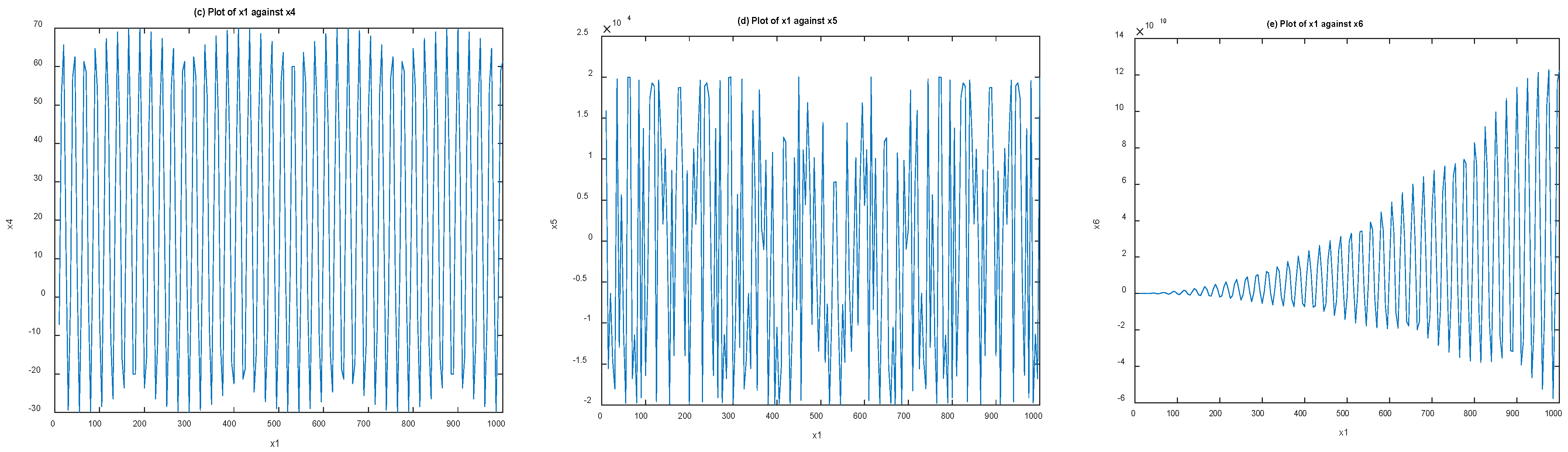
A parametric study is performed to observe how a change in the variables affect the output of the Sine-Gordon wave model. The variables and constants and for = 1:0.5:100 were maintained while the division of the scale of the wavelength was reduced from = 1:0.5:100 to = 1:5:100 to observe how the characteristics of the output wave would change. Based on the result of the simulations, the outputs of , and significantly changed, as shown in Figure 3c–e. appears to have introduced the highest interference, as shown in Figure 3d, although it was superimposed at the output, as shown in Figure 3e.
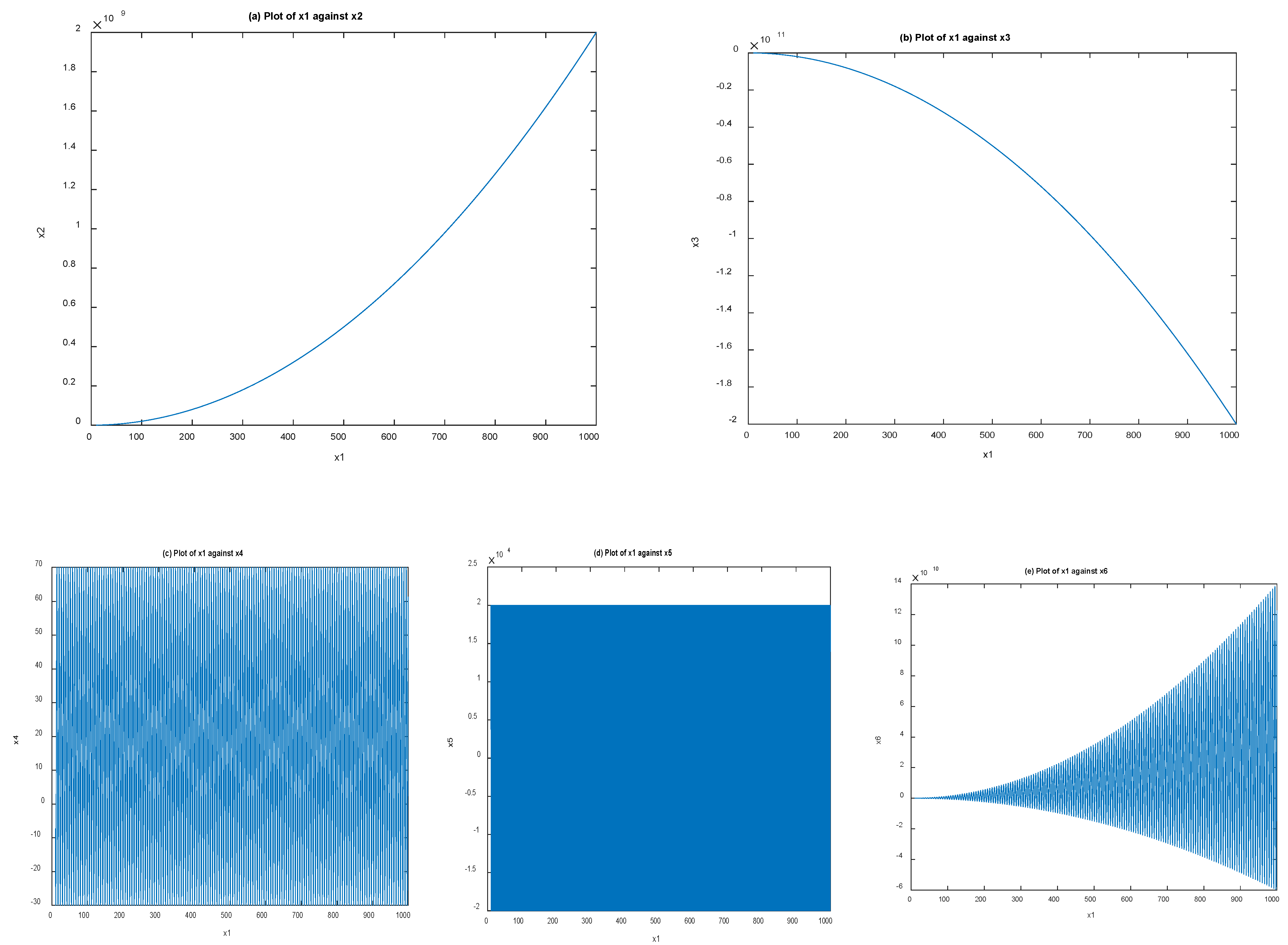
Again, the variables and constants and for = 1:0.5:100 were maintained while the scale of the divisions of the wavelength was increased from = 1:0.5:100 to = 1:0.0005:100 to observe how the characteristics of the output wave would change over a larger scope. There was a significant increase in the frequency of the wave, as shown in the outputs of , , and as visualized in Figure 4c–e. Still, the amplitude of the wave was virtually bounded by the two quadratic functions (Figure 4a,b) with the resultant amplitude increasing progressively, as shown in Figure 4e. This implies that the resultant discontinuity of the two quadratic functions, when visualized from the relationship between and did not eliminate their effects as they constrained the amplitude of the output wave even in their discontinuous states.
In addition to changing the wavelength of the sine functions over the range of other parameters can be adjusted so that their effects can be visualized. With = 1:0.5:100, , and the effect of the change in and in the characteristics of the wave was visualized. Although the scale of the wavelength in Figure 2 and Figure 5 were the same, the output waves in Figure 2e and Figure 5e differ significantly in their frequency when and changed. Based on the analysis of the outputs, the reduced frequency was caused by the effects seen in Figure 2c and Figure 5c, due to . In all the cases, there was an increasing amplitude because of the two quadratic input functions.
From the foregoing analysis in this section, the CBM approach has been used to demonstrate how a hypothetical SoTE including the Sine-Gordon equation was solved to the satisfaction of research objective 2. Also, parametric analysis, which showed how the wavelength and the amplitude responds to the change in the variables, satisfy the research objective 3.
4. Application of SoTE in Photovoltaic and Thermophotovoltaic Modelling and Simulation
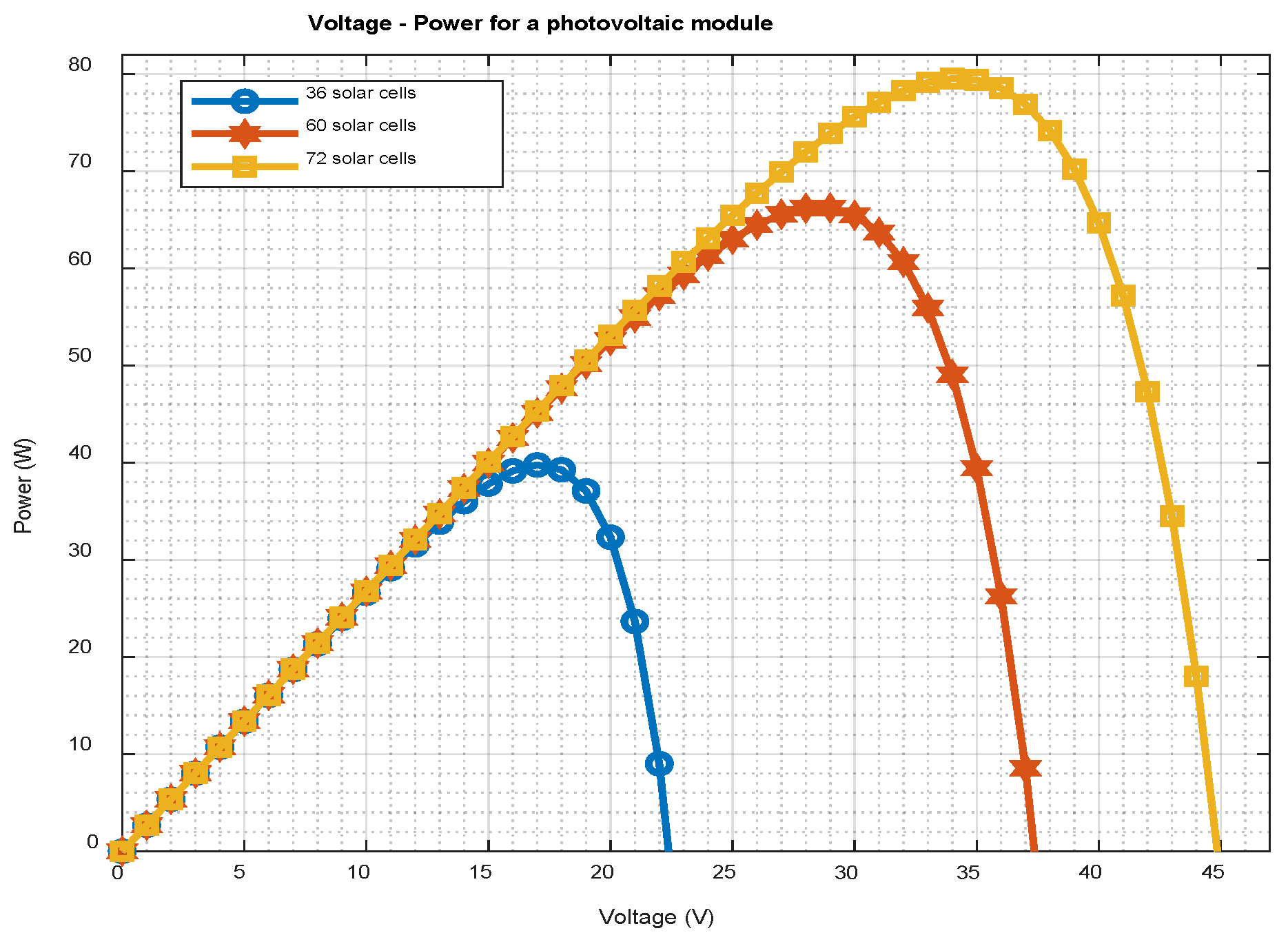
This section presents the application of the CBM approach for modelling and simulation of photovoltaic and thermophotovoltaic systems, pursuant the achievement of objective 4. The photovoltaic and thermophotovoltaic modelling and simulation involves a SoTE because the computation of the output voltage of the PV cells involves a transcendental function [16,24,25]. Equation (2) presents the functions that have been used to create a predictive model for power generation characteristics of the PV module. The inter-relationships between the equations are further highlighted. Bandgap function [26] is an input function in calculating the saturation current function ( [27]. The photocurrent function () [28] is an input function for calculating the output current of the PV (). The typical problem that qualifies this to be a SoTE is that the output voltage () is within the function which is already defining the output current [29]. In order to compute the output power of PV (, the function is iterated over a range of the voltage [16].
As an example, the effect of increasing number of solar cells in series () from 36 to 72 cells is simulated and presented in Figure 6. The open circuit voltage increased as the number of cells increases leading to an increased maximum power point of the system.
Furthermore, the SoTE in Equation (2) which represents solar photovoltaic generation can be utilized to create a thermophotovoltaic model [14]. The insolation (G) can be replaced by Steffan–Boltzmman’s radiation, where the thermal heat flux is from an artificial source with unique radiation surface characteristics. The utility of the CBM approach is the opportunity to adapt the algorithm for implementing SoTE to the specific problem under investigation. In the instant case of the application of CBM approach to implement a numerical solution for SoTE encountered in photovoltaics, two illustrations are hereby highlighted. Equation (2) acted as the power output in the integration of solar, thermal, and electrical exergies of a photovoltaic module, as shown in Equation (3).
Apart from using solar radiation to generate excitation in PV cells, there are increasing research efforts to use sources of heat to generate radiative heat transfer that can cause excitations in PV cells. Regardless, thermophotovoltaic systems still depend on the physics of photovoltaic power generation except that thermophotovoltaic systems are not limited by the risks associated with the intermittency of solar radiation [30]. Equation (4) shows a numerical integration of radiative heat transfer, power density output, and thermal losses in the core of a thermophotovoltaic system [31].
Both Equations (3) and (4) are SoTEs and their solutions were facilitated by using CBM approach. The two models are crucial models for investigating the thermodynamics of photovoltaics and thermophotovoltaics.
5. Conclusions
This study provides detailed steps on how the CBM approach can be used to solve SoTE with multi-functions and multi-variables. To formulate the steps, a hypothetical SoTE including Sine-Gordon equations was used to illustrate the steps for solving a SoTE. Also, a parametric analysis was performed to investigate how a change in the variables affected the superposition of the waves, the wavelength, and the amplitude. From the results of the simulations, the amplitude, wavelength, and frequency of the output wave reflects the changes in the parameters and variables of the SoTE. This means that the properties of the Sine-Gordon wave were altered when the variables and parameters in the CB model of the waves were adjusted. The application of the CBM approach in the modelling and simulation of photovoltaic and thermophotovoltaic systems was presented as practical application of CBM approach in solving a complex SoTE. In conclusion, more functions and variables of physical systems or phenomena can be added during mathematical modelling of problems exhibiting the characteristics of a SoTE, using the steps outlined in this study.
Author Contributions
Conceptualization, C.O.; methodology, C.O., C.A., and A.N.; software, C.O.; validation, C.O., C.A., and A.T.; formal analysis, C.O.; investigation, C.O.; resources, C.A. and A.N.; data curation, C.O.; writing—original draft preparation, C.O. and C.A.; writing—review and editing, C.A. and A.N.; visualization, C.O.; supervision, A.T., C.A. and A.N.; project administration, C.O.; funding acquisition, C.O. All authors have read and agreed to the published version of the manuscript.
Funding
This research was funded by the Petroleum Technology Development Fund (PTDF) Nigeria number PTDF/ED/PHD/OC/1078/17.
Institutional Review Board Statement
Not applicable.
Informed Consent Statement
Not applicable.
Data Availability Statement
Data associated with this research is available at request.
Conflicts of Interest
The authors declare no conflict of interest.
Nomenclature
| A | ideality constant |
| CBM | code-based modelling |
| CB | code-based |
| bandgap energy | |
| output current of PV module | |
| photocurrent | |
| saturation current of PV module | |
| short circuit current of PV module | |
| k | Boltzmann’s const. (1.38 × 10⁻²³ J/K) |
| MPP | maximum power point |
| number of solar cells in series | |
| number of solar cells in parallel | |
| output power of PV module | |
| PV | photovoltaic |
| q | electron charge (1.602 × 10⁻¹⁹ C) |
| SoTE | system of transcendental equations |
| STC | standard test condition (25 °C, 1000 W/m2, AM 1.5) |
| T | temperature |
| TE | transcendental equation |
| open circuit voltage | |
| Greek symbols | |
| α | solar cell material constant |
| β | solar cell material constant |
| Subscripts | |
| cell | solar cell |
| ph | photon |
| pv | photovoltaic |
| ref | reference |
References
- Luck, R.; Stevens, J.W. Explicit Solutions for Transcendental Equations. SIAM Rev. 2002, 44, 227–233. [Google Scholar] [CrossRef]
- Zhang, S.; Zhu, C.; Gao, Q. Numerical Solution of High-Dimensional Shockwave Equations by Bivariate Multi-Quadric Quasi-Interpolation. Mathematics 2019, 7, 734. [Google Scholar] [CrossRef] [Green Version]
- Luck, R.; Zdaniuk, G.J.; Cho, H. An Efficient Method to Find Solutions for Transcendental Equations with Several Roots. Int. J. Eng. Math. 2015, 2015, 1–4. [Google Scholar] [CrossRef] [Green Version]
- Zaguskin, V.L. Handbook of Numerical Methods for the Solution of Algebraic and Transcendental Equations; Pergamon Press: Oxford, UK, 1961. [Google Scholar]
- Jeswal, S.; Chakraverty, S. Solving Transcendental Equation Using Artificial Neural Network. Appl. Soft Comput. 2018, 73, 562–571. [Google Scholar] [CrossRef]
- Boyd, J.P. Computing the Zeros, Maxima and Inflection Points of Chebyshev, Legendre and Fourier series: Solving Tran-Scendental Equations by Spectral Interpolation and Polynomial Rootfinding. J. Eng. Math. 2006, 56, 203–219. [Google Scholar] [CrossRef]
- Ruan, S.; Wei, J. On the Zeros of Transcendental Functions with Applications to Stability of Delay Differential Equations with Two Delays. Dyn. Contin. Discret. Impuls. Syst. Ser. A Math. Anal. 2003, 6, 863–874. [Google Scholar]
- Luo, Q.; Wang, Z.; Han, J. A Padé Approximant Approach to Two Kinds of Transcendental Equations with Applications in Physics. Eur. J. Phys. 2015, 36, 35030. [Google Scholar] [CrossRef] [Green Version]
- Ruggiero, C.M. Solution of Transcendental and Algebraic Equations with Applications to Wave Propagation in Elastic Plates; Naval Research Lab: Washington, DC, USA, 1981. [Google Scholar]
- Maheshwari, A.K. A Fourth Order Iterative Method for Solving Nonlinear Equations. Appl. Math. Comput. 2009, 211, 383–391. [Google Scholar] [CrossRef]
- Falnes, J. Complex Zeros of a Transcendental Impedance Function. J. Eng. Math. 1968, 2, 389–401. [Google Scholar] [CrossRef]
- Wang, D.; Jung, J.-H.; Biondini, G. Detailed Comparison of Numerical Methods for the Perturbed Sine-Gordon Equation with Impulsive Forcing. J. Eng. Math. 2014, 87, 167–186. [Google Scholar] [CrossRef]
- Cao, Q.; Djidjeli, K.; Price, W.G.; Twizell, E.H. Computational Methods for Some Non-Linear Wave Equations. J. Eng. Math. 1999, 35, 323–338. [Google Scholar] [CrossRef]
- Ogbonnaya, C.; Turan, A.; Abeykoon, C. Numerical Integration of Solar, Electrical and Thermal Exergies of Photovoltaic Module: A Novel Thermophotovoltaic Model. Sol. Energy 2019, 185, 298–306. [Google Scholar] [CrossRef]
- Ogbonnaya, C.; Turan, A.; Abeykoon, C. Novel Thermodynamic Efficiency Indices for Choosing an Optimal Location for Large-Scale Photovoltaic Power Generation. J. Clean. Prod. 2020, 249, 119405. [Google Scholar] [CrossRef]
- Ogbonnaya, C.; Turan, A.; Abeykoon, C. Robust Code-Based Modeling Approach for Advanced Photovoltaics of the Future. Sol. Energy 2020, 199, 521–529. [Google Scholar] [CrossRef]
- Papalambros, P.Y.; Wilde, D.J. Principles of Optimal Design—Modeling and Computation. Math. Comput. 1992, 59, 726. [Google Scholar] [CrossRef]
- Slowik, A.; Kwasnicka, H. Evolutionary Algorithms and their Applications to Engineering Problems. Neural Comput. Appl. 2020, 32, 12363–12379. [Google Scholar] [CrossRef] [Green Version]
- Petela, R. Exergy of Undiluted Thermal Radiation. Sol. Energy 2003, 74, 469–488. [Google Scholar] [CrossRef]
- Abed, S.S.; Taresh, N.S. Abed on Stability of Iterative Sequences with Error. Mathematics 2019, 7, 765. [Google Scholar] [CrossRef] [Green Version]
- Aleshin, N.; Kamenskii, V.; Mogil’Ner, L. Solution of a Transcendental Equation Encountered in Diffraction Problems. J. Appl. Math. Mech. 1983, 47, 139–141. [Google Scholar] [CrossRef]
- Sun, Y. New Exact Traveling Wave Solutions for Double Sine–Gordon Equation. Appl. Math. Comput. 2015, 258, 100–104. [Google Scholar] [CrossRef]
- Porubov, A.; Fradkov, A.; Andrievsky, B. Feedback Control for some Solutions of the Sine-Gordon Equation. Appl. Math. Comput. 2015, 269, 17–22. [Google Scholar] [CrossRef]
- Ogbonnaya, C.; Abeykoon, C.; Damo, U.; Turan, A. The Current and Emerging Renewable Energy Technologies for Power Generation in Nigeria: A Review. Therm. Sci. Eng. Prog. 2019, 13, 100390. [Google Scholar] [CrossRef]
- Ogbonnaya, C.; Turan, A.; Abeykoon, C. Energy and Exergy Efficiencies Enhancement Analysis of Integrated Photovoltaic-Based Energy Systems. J. Energy Storage 2019, 26, 101029. [Google Scholar] [CrossRef]
- Ünlü, H. A Thermodynamic Model for Determining Pressure and Temperature Effects on the Bandgap Energies and other Properties of Some Semiconductors. Solid-State Electron. 1992, 35, 1343–1352. [Google Scholar] [CrossRef]
- Muhammad, F.F.; Yahya, M.Y.; Hameed, S.S.; Aziz, F.; Sulaiman, K.; Rasheed, M.A.; Ahmad, Z. Employment of Single-Diode Model to Elucidate the Variations in Photovoltaic Parameters Under Different Electrical and Thermal Conditions. PLoS ONE 2017, 12, e0182925. [Google Scholar] [CrossRef] [PubMed] [Green Version]
- Bellia, H.; Youcef, R.; Fatima, M. A Detailed Modeling of Photovoltaic Module Using MATLAB. NRIAG J. Astron. Geophys. 2014, 3, 53–61. [Google Scholar] [CrossRef] [Green Version]
- Zeitouny, J.; Katz, E.A.; Dollet, A.; Vossier, A. Band Gap Engineering of Multi-Junction Solar Cells: Effects of Series Resistances and Solar Concentration. Sci. Rep. 2017, 7, 1–9. [Google Scholar] [CrossRef] [Green Version]
- Ogbonnaya, C.; Abeykoon, C.; Nasser, A.; Ume, C.; Damo, U.; Turan, A. Engineering Risk Assessment of Photovoltaic-Thermal-Fuel Cell System Using Classical Failure Modes, Effects and Criticality Analyses. Clean. Environ. Syst. 2021, 2, 100021. [Google Scholar] [CrossRef]
- Ogbonnaya, C.; Abeykoon, C.; Nasser, A.; Turan, A. Radiation-Thermodynamic Modelling and Simulating the Core of a Thermophotovoltaic System. Energies 2020, 13, 6157. [Google Scholar] [CrossRef]
Figure 1.
Flowchart for implementing the CBM approach for solving SoTEs.
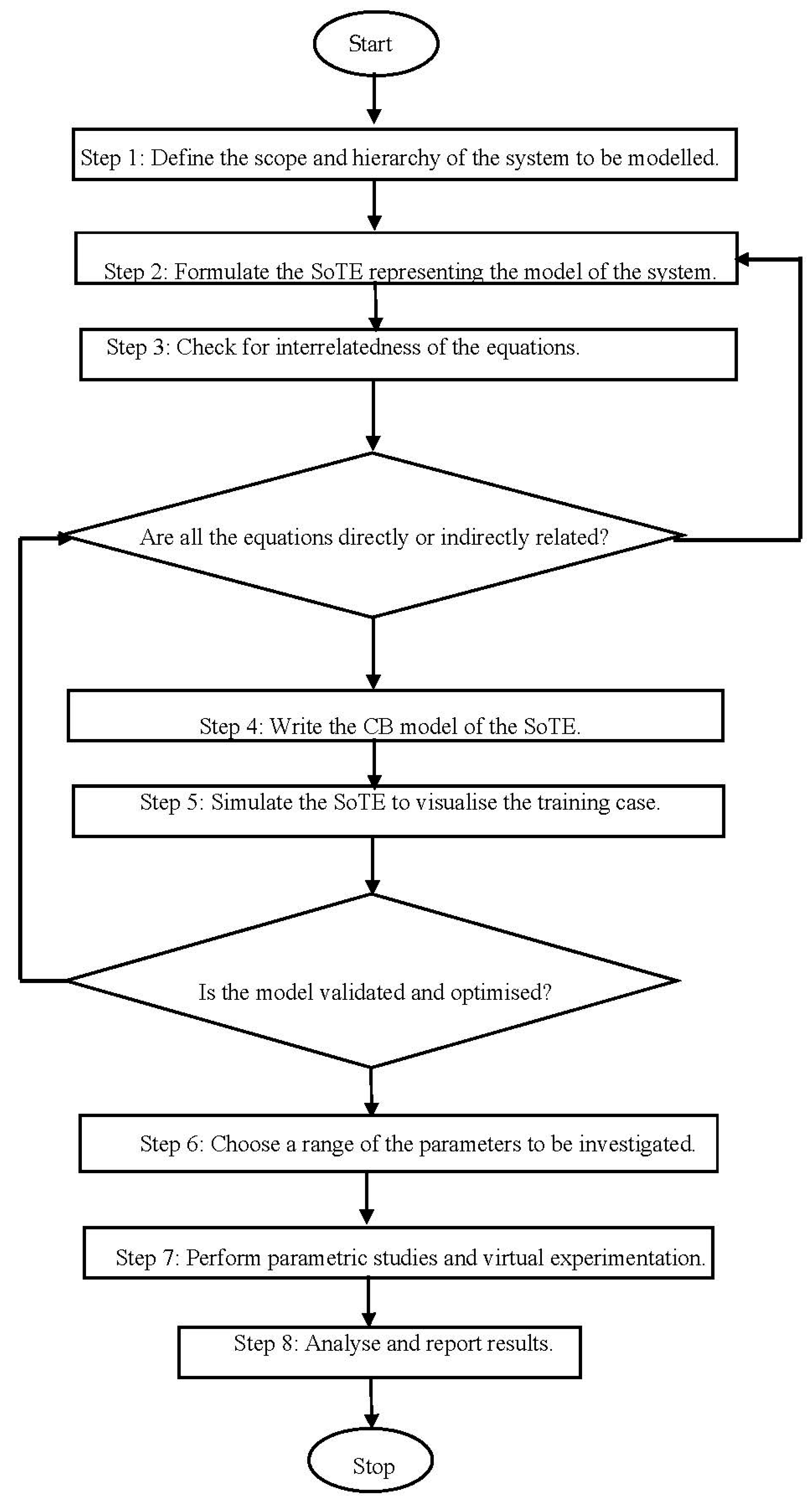
Figure 2.
Simulation of the CB model of SoTE for = 1:0.5:100. (a)input quadratic function, (b) input quadratic function, (c) resultant polynomial function, (d) induced interference (e) output wave function.
Figure 2.
Simulation of the CB model of SoTE for = 1:0.5:100. (a)input quadratic function, (b) input quadratic function, (c) resultant polynomial function, (d) induced interference (e) output wave function.
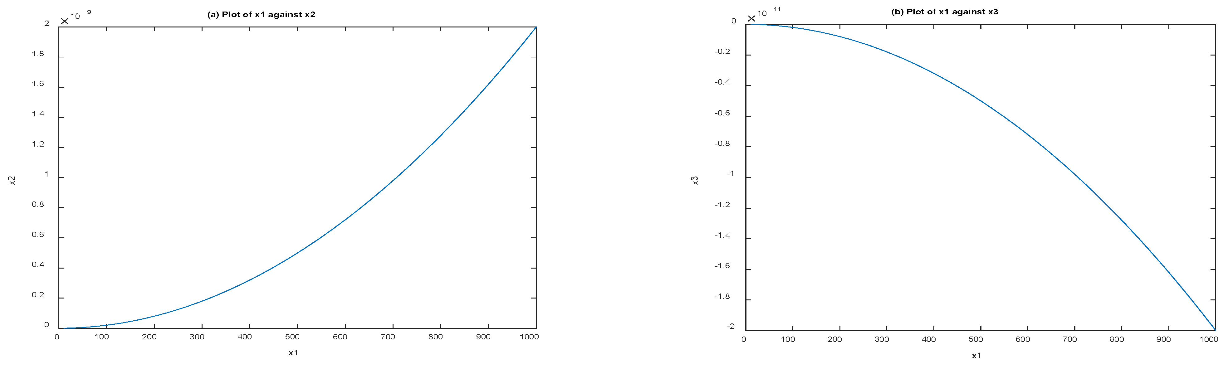

Figure 3.
Simulation of the CB model of SoTE for = 1:5:100. (a)input quadratic function, (b) input quadratic function, (c) resultant polynomial function, (d) induced interference (e) output wave function.
Figure 3.
Simulation of the CB model of SoTE for = 1:5:100. (a)input quadratic function, (b) input quadratic function, (c) resultant polynomial function, (d) induced interference (e) output wave function.
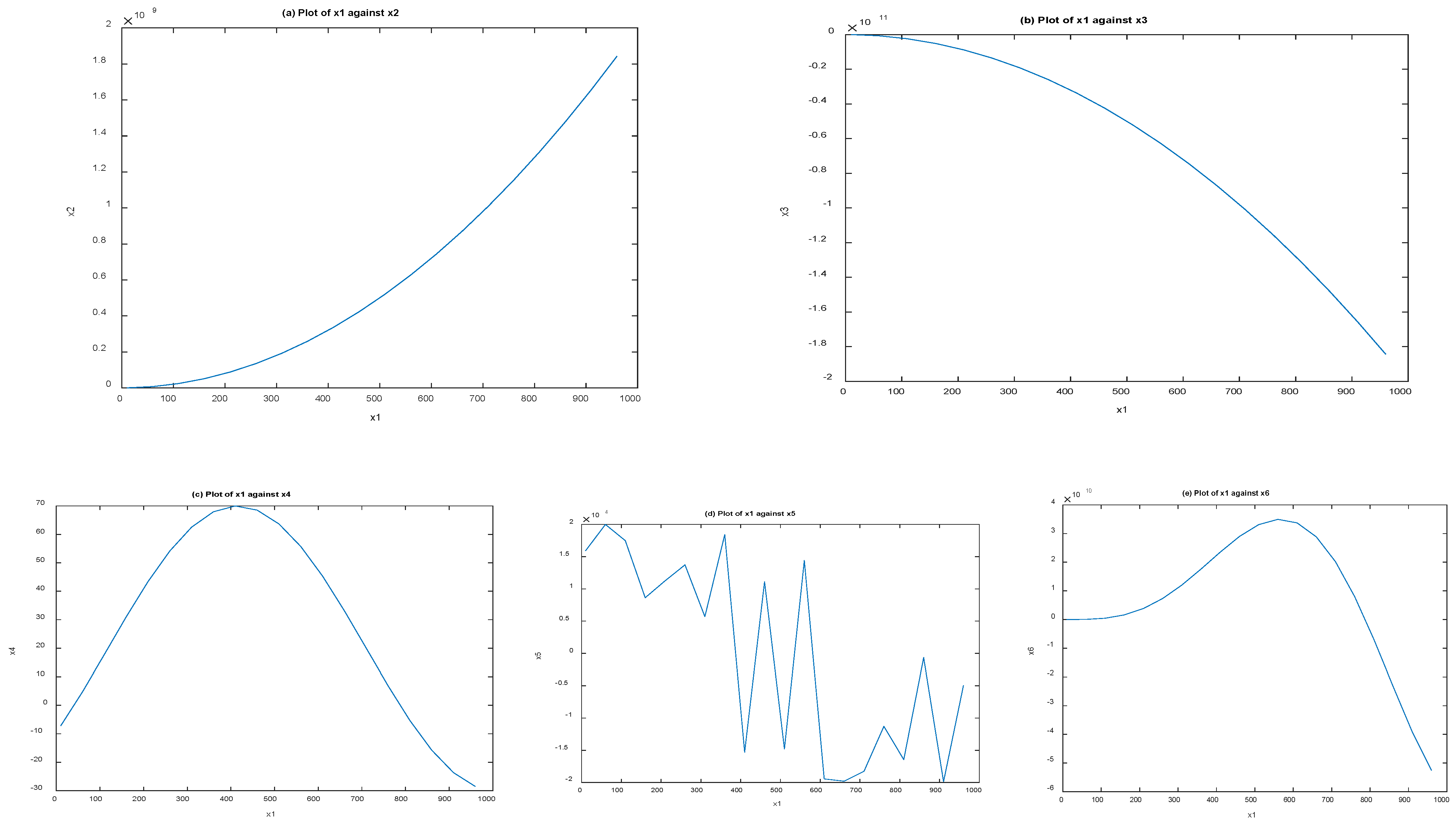
Figure 4.
Simulation of the CB model of SoTE for = 1:0.0005:100. (a)input quadratic function, (b) input quadratic function, (c) resultant polynomial function, (d) induced interference (e) output wave function.
Figure 4.
Simulation of the CB model of SoTE for = 1:0.0005:100. (a)input quadratic function, (b) input quadratic function, (c) resultant polynomial function, (d) induced interference (e) output wave function.

Figure 5.
Simulation of the CB model of SoTE for = 1:0.5:100 with variation in and . (a)input quadratic function, (b) input quadratic function, (c) resultant polynomial function, (d) induced interference (e) output wave function.
Figure 5.
Simulation of the CB model of SoTE for = 1:0.5:100 with variation in and . (a)input quadratic function, (b) input quadratic function, (c) resultant polynomial function, (d) induced interference (e) output wave function.
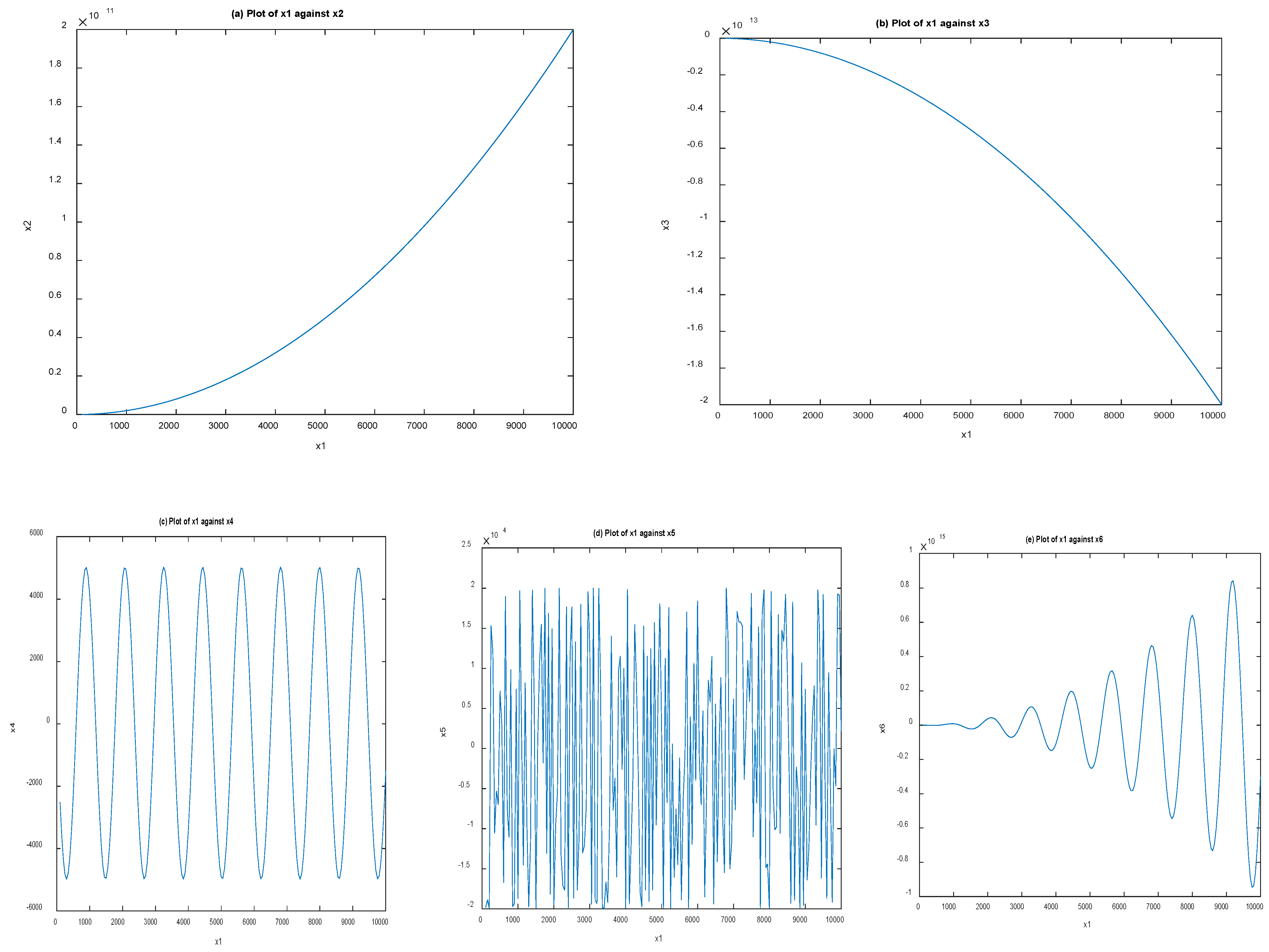
Figure 6.
CB model of photovoltaic module to predict maximum power points as the number of solar cells changes.
Figure 6.
CB model of photovoltaic module to predict maximum power points as the number of solar cells changes.
Publisher’s Note: MDPI stays neutral with regard to jurisdictional claims in published maps and institutional affiliations. |
© 2021 by the authors. Licensee MDPI, Basel, Switzerland. This article is an open access article distributed under the terms and conditions of the Creative Commons Attribution (CC BY) license (https://creativecommons.org/licenses/by/4.0/).
Share and Cite
MDPI and ACS Style
Ogbonnaya, C.; Abeykoon, C.; Nasser, A.; Turan, A. A Computational Approach to Solve a System of Transcendental Equations with Multi-Functions and Multi-Variables. Mathematics 2021, 9, 920. https://doi.org/10.3390/math9090920
AMA Style
Ogbonnaya C, Abeykoon C, Nasser A, Turan A. A Computational Approach to Solve a System of Transcendental Equations with Multi-Functions and Multi-Variables. Mathematics. 2021; 9(9):920. https://doi.org/10.3390/math9090920
Chicago/Turabian StyleOgbonnaya, Chukwuma, Chamil Abeykoon, Adel Nasser, and Ali Turan. 2021. "A Computational Approach to Solve a System of Transcendental Equations with Multi-Functions and Multi-Variables" Mathematics 9, no. 9: 920. https://doi.org/10.3390/math9090920
Note that from the first issue of 2016, this journal uses article numbers instead of page numbers. See further details here.