
On the Oscillatory Properties of Solutions of Second-Order Damped Delay Differential Equations
by
 ,
,
Awatif A. Hendi
1, 
Osama Moaaz
2,3 ,
,
Clemente Cesarano
3,*, 
Wedad R. Alharbi
4 and
Mohamed A. Abdou
5 1
Department of Physics, College of Science, Princess Nourah bint Abdulrahman University, Riyadh, Saudi Arabia
2
Department of Mathematics, Faculty of Science, Mansoura University, Mansoura 35516, Egypt
3
Section of Mathematics, International Telematic University Uninettuno, CorsoVittorio Emanuele II, 39, 00186 Roma, Italy
4
Physics Department, Faculty of Science, University of Jeddah, Jeddah, Saudi Arabia
5
Department of Physics, College of Sciences, University of Bisha, P.O. Box 344, Bisha 61922, Saudi Arabia
*
Author to whom correspondence should be addressed.
Mathematics 2021, 9(9), 1060; https://doi.org/10.3390/math9091060
Submission received: 31 March 2021
/
Revised: 29 April 2021
/
Accepted: 5 May 2021
/
Published: 9 May 2021
(This article belongs to the Special Issue Orthogonal Polynomials and Special Functions)
Abstract
:In the work, a new oscillation condition was created for second-order damped delay differential equations with a non-canonical operator. The new criterion is of an iterative nature which helps to apply it even when the previous relevant results fail to apply. An example is presented in order to illustrate the significance of the results.
1. Introduction
In this study, we focus on studying the oscillatory properties of solutions to the delay differential equation (DDE)
where , and under the following hypotheses:
Hypothesis 1 (H1).
is a quotient of two odd integers.
Hypothesis 2 (H2).
for , and on any half-line .
Hypothesis 3 (H3).
, , and .
By a solution of (1), we go to a with and for and satisfies (1) on . A solution of (1) is called non-oscillatory if it is eventually positive or eventually negative; otherwise, it is called oscillatory.
DDEs, as a subclass of the functional differential equation (FDE), take into account the system’s past, allowing for more accurate and efficient future prediction while also describing certain qualitative phenomena such as periodicity, oscillation, and instability. The concept of delay incorporation into systems is now proposed to play an important role in modeling when representing the time it takes to complete certain secret processes, see [1]. DDE theory has improved our understanding of the qualitative behavior of their solutions and has a wide range of applications in mathematical biology and other fields. DDE nonlinearity and sensitivity analysis has been extensively studied in recent years in a variety of fields, see [2,3,4,5,6].
The problem of determining oscillation criteria for specific FDEs has been a very active research field in the recent decades, and many references and summaries of known results can be found in the monographs by Agarwal et al. [7,8] and Gyori and Ladas [9].
The following is a review of the most important results that dealt with the oscillatory behavior of solutions of DDEs with damping term.
By many authors, the oscillation of the ordinary differential equation with damping term
has been investigated. The existence of a damping term in differential equations necessarily requires an improved approach at the study of oscillatory behavior. Among the works that dealt with the oscillation of (2) are, for example, Grace [10,11], Grace and Lalli [12,13], Grace et al. [14], Kirane and Rogovechenkov [15], Li and Agarwal [16], Li and Zhang [17], Rogovechenkov [18], Wong [19], and Yan [20]. However, the common restriction is required in all previous works. Grace [21] studied the oscillation of DDE
with the canonical case.
Theorem 1.
Theorem 2.
Theorem 3.
In an attempt to reduce the number of possible possibilities for the sign of derivatives of positive solutions, researchers study the DDEs in the canonical case, which often excludes the existence of positive decreasing solutions. On the other hand, in the noncanonical case, one of these possibilities is that the positive solutions are decreasing. The main reason for the difficulty of studying positive decreasing solutions is the probability of their convergence to zero, and this probability prevents the use of one of the most important relationships between derivatives that allows to reduce the order of the equation. It has also been noted that the conditions resulting from the exclusion of positive decreasing solutions have the largest effect on the oscillation criteria. Therefore, the main objective of this work is to study the oscillatory behavior of DDE (1) in the noncanonical case
The technique used is based on obtaining criteria of an iterative nature through establishing more sharp estimates for the . The iterative nature of the criteria allows us to apply them more than once, even when the other criteria fail.
2. Main Results
For ease of presentation of results, we present the next notations:
Lemma 1.
Assume that and
Then
Proof.
Assume that . Then, we have that and are positive for all , for some . Therefore, it follows from (1) that
Hence, is of one sign. Suppose the contrary that for for some . Thus, there is a such eventually that . Integrating (11) from to ∞, we obtain
From (10) and the fact that , we have that
which with (12) gives a contradiction, and so , eventually.
Now, we have that is positive decreasing, and then . Suppose that . Then, eventually. Hence, integrating (11) from to l, we obtain
or
Integrating (13) from to ∞, we arrive at
which contradicts (10). Then, converges to zero.
Finally, we have
Therefore,
The proof is complete. □
Lemma 2.
Proof.
Assume that . Then, we have that and are positive for all , for some . From Lemma 1, we have that , , (11) and (15) hold. Using (15) and the fact that , we get that
From (11), (17) and (19), we have
Firstly, at , integrating (21) from to l, we obtain
From , we have that converges to , and then
eventually. Thus, from (22), we obtain
This implies
Now, is positive decreasing, and then . Suppose that . Then, eventually. If we define the function
then it follows from that , and
which, with (21) and (23) and the fact that , gives
Integrating this inequality from to ∞, we obtain
Letting , we arrive at a contradiction, and then converges to zero.
Next, from (21), we have
Integrating this inequality from l to ∞ and using , we obtain
Therefore,
That is, and are satisfied for
Secondly, proceeding to the next induction step, we suppose that and hold for some . Using , (20) becomes
Integrating this inequality from to l and using , we find
From (16), , eventually. Thus, (24) turn into
Since converges to zero, we have that
eventually. Thus,
and hence
Proceeding exactly as in the previous step (at ), we can verify and .
The proof is complete. □
Theorem 4.
Proof.
If we suppose that (1) has a solution , then, from Lemma 2, we have is decreasing and is increasing. Therefore, for all , this is a contradiction. The proof is complete. □
Theorem 5.
Proof.
If we suppose that (1) has a solution , then, from Lemma 2, we have that , and (20) hold, for all . Now, we define the function
As in the proof of Lemma 1, we have that (15) holds, and so , eventually. Thus,
Hence, from (20), we obtain
Taking the fact that into account, we obtain
and then
Thus, from (26), is a positive solution of the delay differential inequality
Using Theorem 1 in [24], the associated delay differential (25) has also a positive solution, which contradicts to the assumptions of the theorem. The proof is complete. □
Corollary 1.
Proof.
It follows from Theorem 2 in [25] that condition (27) implies oscillation of (25). □
Example 1.
3. Conclusions
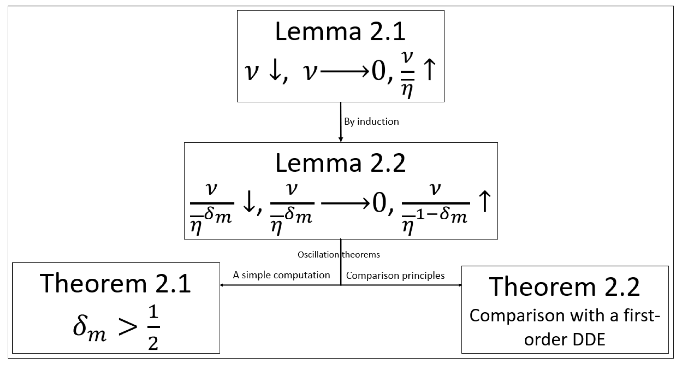
We have greatly less results for DDEs with noncanonical operator than for the DDEs with canonical operator. So, in this work, new sufficient conditions for the oscillation of second-order damped DDE with noncanonical operator (1) are established. By inferring and improving some properties of positive solutions, we establish oscillation criteria of an iterative nature. For an overview of the main results, see Figure 1. It would be interesting to extend our results to neutral DDEs.
Author Contributions
All authors contributed equally to this work. All authors have read and agreed to the published version of the manuscript.
Funding
This research was funded by the Deanship of Scientific Research at Princess Nourah bint Abdulrahman University through the Fast-track Research Funding Program.
Institutional Review Board Statement
Not applicable.
Informed Consent Statement
Not applicable.
Data Availability Statement
Not applicable.
Acknowledgments
The authors present their sincere thanks to the editors and two anonymous referees. This research was funded by the Deanship of Scientific Research at Princess Nourah bint Abdulrahman University through the Fast-track Research Funding Program.
Conflicts of Interest
There are no competing interest.
References
- Hale, J.K. Partial neutral functional differential equations. Rev. Roum. Math. Pures Appl. 1994, 39, 339–344. [Google Scholar]
- Bocharov, G.A.; Rihan, F.A. Numerical modelling in biosciences using delay differential equations. J. Comput. Appl. Math. 2000, 125, 183–199. [Google Scholar] [CrossRef] [Green Version]
- Rakkiyappan, R.; Velmurugan, G.; Rihan, F.; Lakshmanan, S. Stability analysis of memristor-based complex-valued recurrent neural networks with time delays. Complexity 2015, 21, 14–39. [Google Scholar] [CrossRef]
- Bahadorinejad, A.; Imani, M.; Braga-Neto, U.M. Adaptive particle filtering for fault detection in partially-observed Boolean dynamical systems. IEEE/ACM Trans. Comput. Biol. Bioinform. 2018, 17, 1105–1114. [Google Scholar] [CrossRef] [PubMed]
- Imani, M.; Ghoreishi, S.F. Partially-Observed Discrete Dynamical Systems. In Proceedings of the American Control Conference (ACC), New Orleans, LA, USA, 26–28 May 2021. [Google Scholar]
- Wenger, J.; Hennig, P. Probabilistic Linear Solvers for Machine Learning. arXiv 2020, arXiv:2010.09691. [Google Scholar]
- Agarwal, R.P.; Grace, S.R.; O’Regan, D. Oscillation Theory for Second Order Linear, Half-Linear, Superlinear and Sublinear Dynamic Equations; Springer Science & Business Media: Berlin/Heidelberg, Germany, 2002. [Google Scholar]
- Agarwal, R.P.; Bohner, M.; Li, W. Non-Oscillation and Oscillation Theory for Functional Differential Equations; Marcel Dekker: New York, NY, USA, 2004. [Google Scholar]
- Gyori, I.; Ladas, G. Oscillation Theory of Delay Differential Equations with Applications; Clarendon Press: Oxford, UK, 1991. [Google Scholar]
- Grace, S.R. Oscillation theorems for second order nonlinear differential equations with damping. Math. Nachr. 1989, 141, 117–127. [Google Scholar] [CrossRef]
- Grace, S.R. Oscillation of nonlinear differential equations of second order. Publ. Math. Debrecen. 1992, 40, 143–153. [Google Scholar] [CrossRef] [Green Version]
- Grace, S.R.; Lalli, B.S. Oscillation theorems for certain second order perturbed nonlinear differential equation. J. Math. Anal. Appl. 1980, 77, 205–214. [Google Scholar] [CrossRef] [Green Version]
- Grace, S.R.; Lalli, B.S. Asymptotic and oscillatory behavior of solutions of a class of second order differential equations with deviating arguments. J. Math. Anal. Appl. 1992, 145, 112–136. [Google Scholar] [CrossRef] [Green Version]
- Grace, S.R.; Lalli, B.S.; Yeh, C.C. Oscillation theorems for nonlinear second order differential equations with a nonlinear damping term. Siam. J. Math. Anal. 1984, 15, 1082–1093. [Google Scholar] [CrossRef]
- Kirane, M.; Rogovechenko, Y.V. Oscillation results for a second order damping differential equations with nonmontonous nonlinearity. J. Math. Anal. Appl. 2000, 250, 118–138. [Google Scholar] [CrossRef] [Green Version]
- Li, W.T.; Agarwal, R.P. Interval oscillation criteria for second order nonlinear differential equations with damping. Comput. Math. Appl. 2000, 40, 217–230. [Google Scholar] [CrossRef] [Green Version]
- Li, W.T.; Zhang, M.Y. Oscillation criteria for second order nonlinear differential equations with damping term. Indian J. Pure Appl. Math. 1999, 30, 1017–1029. [Google Scholar]
- Rogovchenko, Y.V. Oscillation theorems for second-order equations with damping. Nonlinear Anal. Theor. 2000, 41, 1005–1028. [Google Scholar] [CrossRef]
- Wong, J.S. On Kamenev-type oscillation theorems for second-order differential equations with damping. J. Math. Anal. Appl. 2001, 258, 244–257. [Google Scholar] [CrossRef]
- Yan, J. Oscillation theorems for second order linear differential equations with damping. Proc. Am. Math. Soc. 1986, 98, 276–282. [Google Scholar] [CrossRef]
- Grace, S.R. On the oscillatory and asymptotic behavior of damping functional differential equations. Math. Jpn. 1991, 36, 220–237. [Google Scholar]
- Saker, S.H.; Pang, P.Y.; Agarwal, R.P. Oscillation theorem for second-order nonlinear functional differential equation with damping. Dyn. Syst. Appl. 2003, 12, 307–322. [Google Scholar]
- Tunc, E.; Kaymaz, A. On oscillation of second-order linear neutral differential equations with damping term. Dyn. Syst. Appl. 2019, 28, 289–301. [Google Scholar] [CrossRef] [Green Version]
- Philos, C.G. On the existence of nonoscillatory solutions tending to zero at ∞ for differential equations with positive delays. Arch. Math. 1981, 36, 168–178. [Google Scholar] [CrossRef]
- Kitamura, Y.; Kusano, T. Oscillation of first-order nonlinear differential equations with deviating arguments. Proc. Am. Math. Soc. 1980, 78, 64–68. [Google Scholar] [CrossRef]
Figure 1.
Schematic diagram for main results.

Table 1.
The first value of which satisfies Condition (29).
| 1 | |||||
| 2 | |||||
| 3 | |||||
| 18 | |||||
| 52 |
Publisher’s Note: MDPI stays neutral with regard to jurisdictional claims in published maps and institutional affiliations. |
© 2021 by the authors. Licensee MDPI, Basel, Switzerland. This article is an open access article distributed under the terms and conditions of the Creative Commons Attribution (CC BY) license (https://creativecommons.org/licenses/by/4.0/).
Share and Cite
MDPI and ACS Style
Hendi, A.A.; Moaaz, O.; Cesarano, C.; Alharbi, W.R.; Abdou, M.A. On the Oscillatory Properties of Solutions of Second-Order Damped Delay Differential Equations. Mathematics 2021, 9, 1060. https://doi.org/10.3390/math9091060
AMA Style
Hendi AA, Moaaz O, Cesarano C, Alharbi WR, Abdou MA. On the Oscillatory Properties of Solutions of Second-Order Damped Delay Differential Equations. Mathematics. 2021; 9(9):1060. https://doi.org/10.3390/math9091060
Chicago/Turabian StyleHendi, Awatif A., Osama Moaaz, Clemente Cesarano, Wedad R. Alharbi, and Mohamed A. Abdou. 2021. "On the Oscillatory Properties of Solutions of Second-Order Damped Delay Differential Equations" Mathematics 9, no. 9: 1060. https://doi.org/10.3390/math9091060
Note that from the first issue of 2016, this journal uses article numbers instead of page numbers. See further details here.