Pricing Decision within an Inventory Model for Complementary and Substitutable Products


1
School of Industrial Engineering, College of Engineering, University of Tehran, Tehran 456311155, Iran
2
Department of Industrial Engineering, Islamic Azad University, South Tehran Branch, Tehran 1584743311, Iran
3
Principal, Kishore Bharati Bhagini Nivedita College, Ramkrishna Sarani, Behala, Kolkata 700060, India
4
Department of Industrial & Management Engineering, Hanyang University, Ansan, Gyeonggi-do 15588, Korea
*
Author to whom correspondence should be addressed.
Mathematics 2019, 7(7), 568; https://doi.org/10.3390/math7070568
Submission received: 30 March 2019
/
Revised: 24 May 2019
/
Accepted: 31 May 2019
/
Published: 26 June 2019
(This article belongs to the Special Issue Application of Optimization in Production, Logistics, Inventory, Supply Chain Management and Block Chain)
Abstract
:A combination of substitutable and complementary products is very important for any business industry to make all-round profit from different aspects. How deterioration affects complementary products or substitutable products is discussed in this study. This study investigates the pricing and inventory decisions for complementary and substitutable items which are deteriorating in nature. Four models are analyzed where the demand of one product is dependent upon the selling price and the price of another product. This paper tries to compute the optimum prices and order quantities to optimize the total profit, which is the main aim. Theoretically, this model is solved by a classical optimization method. Numerical examples demonstrate the applicability of this model. Results conclude that the total profit is dependent on the degree of substitutability and complementarity. A sensitivity analysis of optimal solutions is given to test the stability of the proposed model.
1. Introduction
Everyday life starts with the use of a toothbrush and toothpaste, which are complementary products. Then, the energy for the whole day is derived from the breakfast where at least one seasonal fruit is mandatory for good health. The seasonal fruit can be replaced by another fruit based on the availability and price and is substitutable product. Whenever the increasing price of one product indicates the increasing sales rate of another product, then those products substitute each other [1]. Increasing the price of one item can help to increase the sale of another substitutable item. For example, Coca-Cola and Pepsi are two substitutable products as both can satisfy the purpose. One customer can buy Pepsi instead of Coca-Cola in any circumstances. Complementary products are used in combination with another product [2]. Single use of any part of complementary products has limited usage. The overall utility is increased whenever both products are used together. The market demand of complementary products depends upon both products [3]. Car and fuel, camera and memory card, toothpaste and brush—these are a few examples of complementary products. A car cannot move without proper fuel, which implies that the car is useless without fuel, and fuel is no longer important if the car is not there. To earn in all aspects, the manufacturer introduces substitutable as well as complementary products in the business. From the perspective of the inventory, complementary products need more storage and inventory, as both products are important. In reality, substitutable products give the manufacturer tough competition, as it is important to choose alternative products very wisely such that it can satisfy the demand as well as the quality of the original product. The pricing factor is the next important thing for substitutable products. The price of the alternative should be less than or equal to the original product. The situation may differ in case of the reverse situation when the alternative’s price is greater than the original price. The situation gets more complicated when the product deteriorates in nature.
There are several researches who focus on substitutable and complementary products, while none of them have investigated both inventory and pricing decisions of the products simultaneously. Moreover, this investigation is done for deteriorating products. In this paper, four models are discussed for pricing and inventory decisions of two types of items, which may be complementary or substitutable, and deteriorating or non-deteriorating. The rest of the present paper is organized as follows: Section 2 presents a literature review, whereas problem definition, notation, and assumptions are defined in Section 3, and the mathematical modeling is presented in Section 4. Numerical examples, a sensitivity analysis, and managerial insights are provided in Section 5. Section 6 concludes the achievements of this proposed model. The last section provides the References of the study.
2. Literature Review
Pricing policy is an important part in the field of supply chain management [4,5,6,7]. Several research articles have been studied on inventory and pricing decisions for single or multi-products inventory models [8,9,10]. However, few of them studied pricing decisions for complementary or substitutable products. In such cases, the price, quality, and durability of the products play a crucial role to attract customers [5,9]. On the other hand, retailers face the cross-selling phenomenon for complementary products. McGillivray and Silver [11] investigated the full substitutability and its effect on total cost within an inventory model. Zhang et al. [12] illustrated an inventory system when the demand of a minor and a major item is correlated with cross-selling. Zhang [13] discussed an inventory problem for multiple products with the inventory replenishment. They proposed a search method which gives a global optimum solution. Yue et al. [14] investigated a duopoly market dealing with complementary products.
An inventory model was discussed by Liu and Yuan [15] for two types of products where the consumption rates of those products are correlated, and the replenishment rates are coordinated. Wei et al. [9] analyzed a non-coordination supply chain management consisting of two manufactures with one retailer for two complementary type products with the help of five different game theories: manufacturer-leader Bertrand, manufacturer-leader Stackelberg, retailer-leader Bertrand, retailer-leader Stackelberg, and Nash game (NG) models. Guchhait et al. [16] studied an advertisement-dependent demand scenario within supply chain management. They used a Stackelberg game policy to solve the model. Shavandi et al. [17] extended the pricing and lot sizing model of Abad [18] for multiple products. They proposed several pricing strategies of multi-products for deteriorating items which may be complementary, substitutable, or independent. The aim of the research was to maximize the profit optimization, along with optimum prices and production quantities.
An inventory model was studied by Balkhi and Benkherouf [19] for deteriorating products. The market demand was stock dependent and time dependent. A procedure was proposed by them to achieve the optimum replenishment schedule. Anjos et al. [20] considered perishable products and presented a continuous pricing strategy where the optimal pricing strategy can be explicitly characterized and easily implemented. Dye [21] extended an inventory model for perishable items with a time-dependent backlog by assuming a price-sensitive demand and variable deterioration with time. In that article, an improved algorithm was proposed by them to find out the optimal selling price of a product and replenishment schedule. Panda et al. [22] considered a single-item economic order quantity (EOQ) model with discounted sale as products were perishable in nature, and the demand was stock dependent. Pang [23] studied optimal dynamic pricing policies and inventory control policies for deteriorating products within a periodic type inventory model. Sarkar and Saren [24] investigated the effect of the trade-credit policy for exponentially deteriorating products. Sarkar et al. [25] developed a two-echelon supply chain model for deteriorating items, where single-setup-multi-delivery (SSMD) transportation policy was adopted.
Sett et al. [26] and Sarkar et al. [27] studied fixed lifetime products and their replenishment policy. The deterioration rate was variable, and the backlog was time dependent. Sarkar et al. [28] applied preservation technology for seasonal deteriorating products while Ullah et al. [29] used the preservation for waste generation. Recycling of the deteriorated products was investigated by Iqbal and Sarkar [30]. The market demand can be affected by the deterioration and a backlog scenario may appear in that case. The service level can help to get rid of this situation [31]. Gürler and Yilmaz [32] studied a supply chain management with two substitutable products in a newsboy problem. Demands for both products were independent, and the aim of the research was to maximize the retailer’s and manufacturer’s profits jointly. Kim and Bell [33] proposed that the production system of a firm sold their products to multiple market segments for a specific period. A price-driven scenario was examined by them, and the effect on the pricing strategy and production capacity of the firm were discussed.
Stavrulaki [34] investigated an inventory model for substitutable products. They explained the combined effect of the demand stimulation for stochastic demand. Karakul and Chan [35] studied the analytical implications of product substitutability and procurement decisions in a newsboy problem with two products. Thereafter, they established the unimodality of the expected profit of their previous work [36] with respect to the procurement and price of quantities. Birge et al. [37] developed an inventory model for substitutable products where market demand follows a uniform distribution. Netessine et al. [38] determined the optimum procurement for multi-substitutable items under exogenous prices of an integrated inventory-pricing problem. Parlar and Goyal [39] developed two integrated production–inventory models of two substitutable products under different prices and assumptions [40]. Tang and Yin [41] discussed an improved procedure to find the optimum selling price within an inventory framework where demand is price sensitive for substitutable products. Xia [42] suggested a two-echelon supply chain model including competitive multiple suppliers and multiple buyers, where each supplier offers one type of substitutable product to the buyers. Netessine et al. [43] discussed about centralized inventory policy where market demand is substitutable. Table 1 gives the contribution from different authors associated with the area of research.
3. Problem Description, Notation, and Assumptions
3.1. Problem Definition
Consider a market where the retailer intends to determine the order quantities of different products. The products may be complementary or substitutable, for which two different scenarios exist.
In case of complementary products, the retailer expects a higher consumption rate of a product when the consumption rate of its complementary product increases and vice versa. Moreover, the demand of every complementary product depends upon the price of the other such that the high price of one of them decreases the demand of the complementary product and vice versa. Obviously, the degree of complementarity between two products, which is between 0 and 1, has the main effect on the changes between their respective demands and prices. In this situation, the retailer determines the optimal order quantity and selling price of each product in such a way that the retailer can maximize the total profit.
In the second scenario, each product can be used instead of another one in the case of substitutable products. In this situation, the retailer faces the situation that the decreasing demand of a substitutable product increases the other product’s demand. The demand of each substitutable product depends upon its own price and the price of another one such that the higher price of one of them increases the demand of its substitutable product and vice versa because the customer intends to use the substitutable product, which has a lower price compared to the other. Generally, the degree of substitutability between two products, which is between 0 and 1, has the main effects on the changes between their demands and prices. Therefore, the retailer should determine the optimum order quantity such that the total profit should maximize.
3.2. Notation
The notation related to this study is given in the Nomenclature section at the end of the study.
3.3. Assumptions
Assumptions are used to formulate the model are as follows:
- A retailer maximizes the profit based on an economic order quantity (EOQ) model. The demand is dependent upon selling prices and lot sizes of two types of products. The demand of two complementary products is dependent upon each product’s selling price and the degree of complementarity.
- After a certain time, products start to deteriorate with a constant deterioration rate. As deterioration is considered in this model, deterioration cost per time unit for the product m is ($ per unit). The deterioration rate of product 1 and product 2 is .
- The degree of complementarity between two products is given by , where and the degree of substitutability between two products is given by d, where .
- The lead time is zero, and there are no shortages for both types of products.
- The time horizon is infinite.
4. Mathematical Model
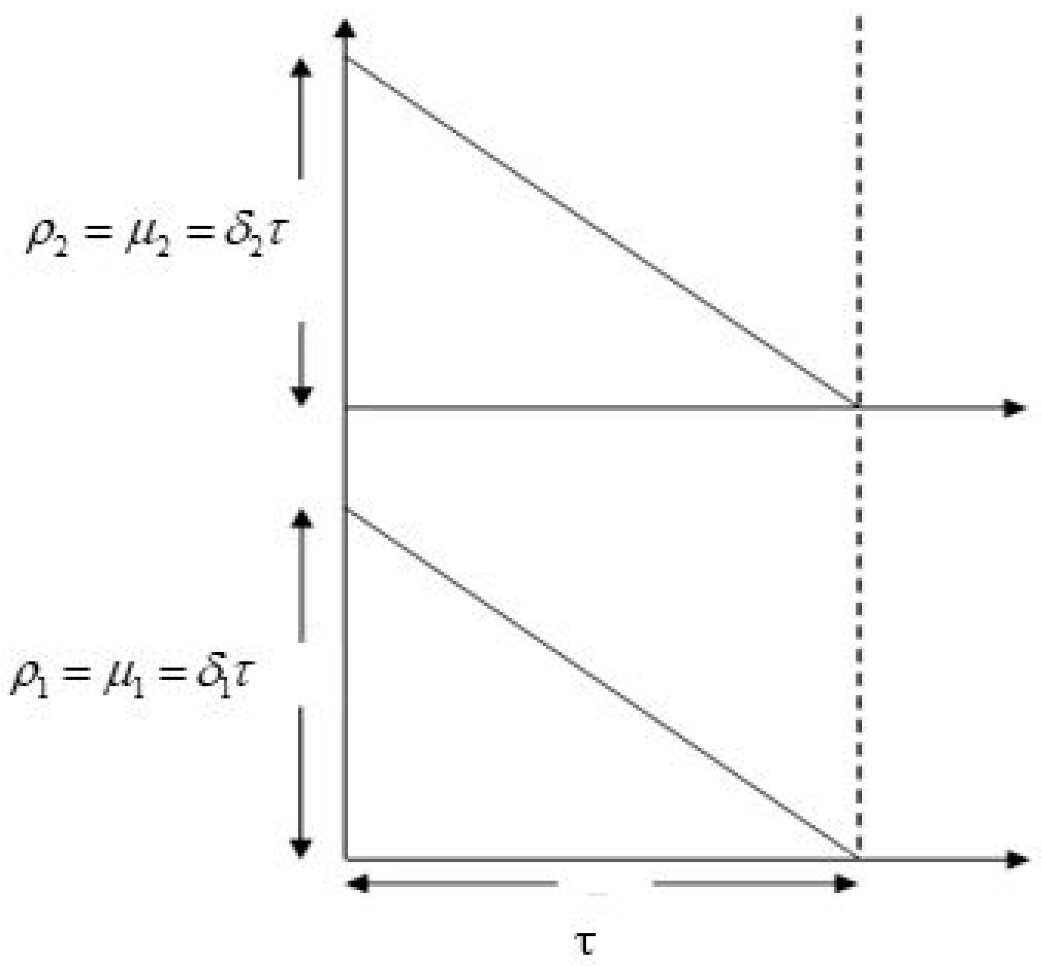
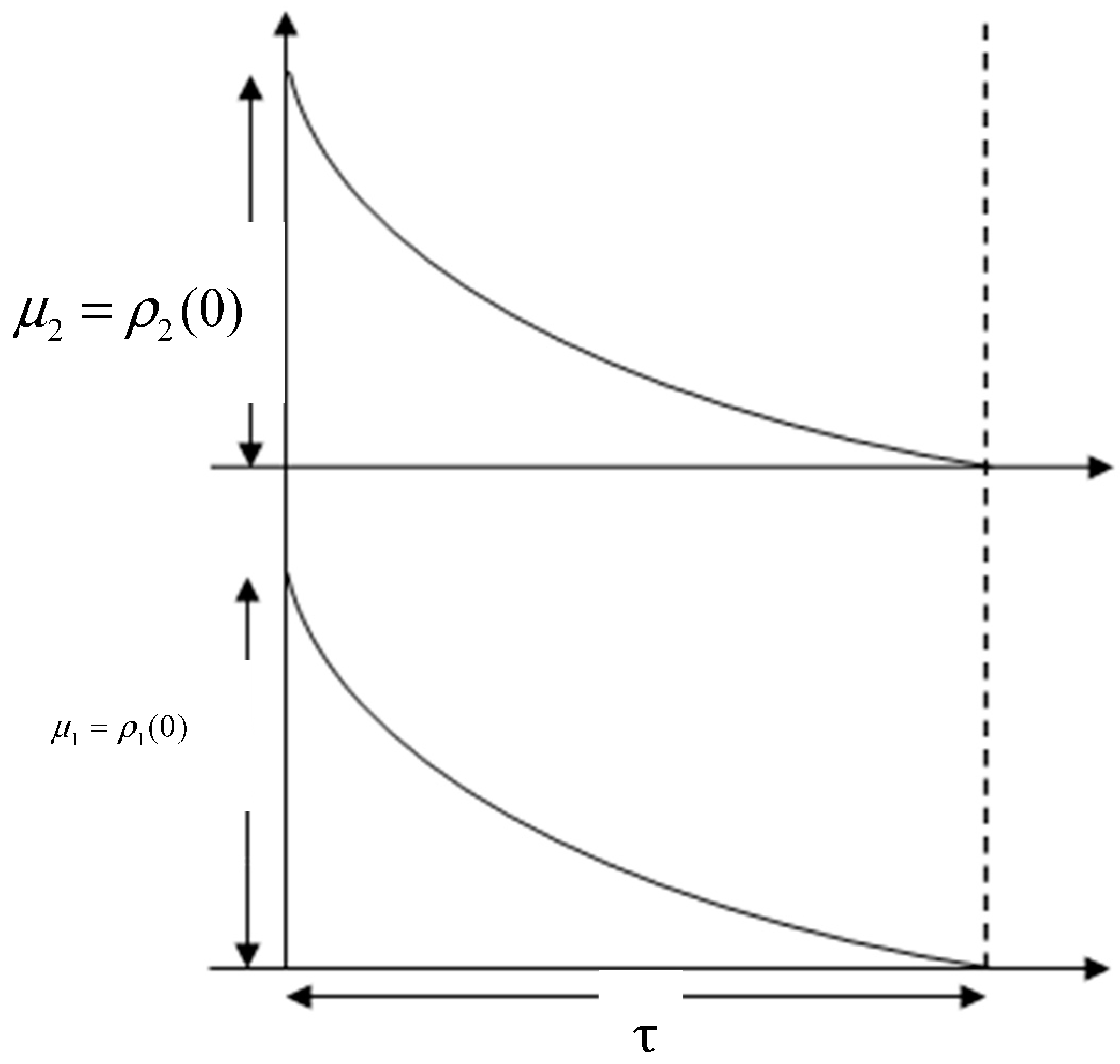
The scenarios for both non-deteriorating (Figure 1) and deteriorating (Figure 2) products are discussed.
In all cases, the aim is to find the optimal values of the order quantity, the cycle length, and selling prices for profit maximization.
4.1. Non-Deteriorating Complementary Products
This section discusses the complementary products when products are of a non-deteriorating type. The demand [35,44] of two complementary products, product 1 and product 2, are
respectively. Here, all parameters () are non-negative. The retailer is trying to obtain the optimal values of decision variables. Therefore, the average profit is
Expression (1) gives the revenue from product 1. Expression (2) explains the revenue from product 2, and Expression (3) defines the summation of ordering costs and holding costs. The purpose is to maximize the profit, using the following theorem:
Theorem 1.
is strictly concave if
Proof.
See Appendix A.
Substituting the values of and within the first order derivative of the Equation (3) with respect to the decision variable τ, one can obtain
The first order derivatives of Equation (3) with respect to the variables and are given by
The required optimum values of and are as given by the following expressions as:
Using Equations (7) and (8) on the right-hand side of Equation (4) and equating them to zero, one can obtain
where
Equation (9) is a cubic polynomial and the discriminant is
According to Δ, the discriminant has three types of values. Δ > 0 gives three real roots of distinct quality, Δ = 0 gives multiple real roots, and Δ < 0 gives one real root and two complex roots. The following improved solution procedure has been developed to solve the problem numerically.
Solution algorithm
- Step 1.
- Using Equations (10)–(12), calculate the coefficients of polynomial shown in Equation (9).
- Step 2.
- All positive real roots of Equation (9) are found by using MATLAB software. Go to the Step (3).
- Step 3.
- Determine the values from Step (2).
- Step 4.
- For all combinations of , obtain the profit and check the concavity clause (Theorem 1). Select the maximum value as an optimal value of the profit. Then the related optimum decision variables are , and .
- Step 5.
- Determine the optimal values of the order quantities using and .
4.2. Non-Deteriorating Substitutable Products
This section discusses about non-deteriorating substitutable products. The demand of two substitutable products, product 1 and product 2, is defined as follows:
where all parameters are non-negative. The average profit is
The following theorem is used to maximize the above profit.
Theorem 2.
is strictly concave
Proof.
See Appendix B.
Now, Equation (16) gives the following expression with respect to the variables τ, , and .
Equations (18) and (19) give the optimum values of and as
Using Equations (20) and (21) on the right-hand side of Equation (17) and equating them to zero, one can obtain
where
According to the discussion about the discriminant of cubic polynomial above, the following solution procedure is suggested for the substitutable products case.
Solution algorithm
- Step 1.
- Using Equations (23)–(25), calculate the coefficients of the polynomial in Equation (22).
- Step 2.
- After finding all possible roots of Equation (22) with the help of MATLAB software, go to the Step (3).
- Step 3.
- From Step 2, determine the values of .
- Step 4.
- For all values of , determine the total profit and check the concavity clause (Theorem 2). Then select the maximum value as the optimum one. The related decision variables associated with the maximum profit are , and .
- Step 5.
- Determine optimal values of order quantities using and .
4.3. Deteriorating Complementary Products
In this case, it is assumed that the retailer is doing the business with two deteriorating complementary products. For both products, the deterioration rates are constant. The differential equation shows that the inventory level changes over time, where . Solving this differential equation yields , and according to Figure 2, the order quantity of each product is equal to . The holding cost is given by
Moreover, the deterioration cost is
The total cost after utilizing the approximation of the Taylor series expansion, , is
The demand of two deteriorating complementary products, product 1 and product 2, is as follows (as defined in Section 4.1):
Finally, the average profit is
To optimize the profit, the following theorem is used.
Theorem 3.
is strictly concave if
Proof.
See Appendix C.
Here, the first order derivative of Equation (31) with respect to T yields
The first order derivatives of the Equation (31) for variables and are given by
Optimum values of the decision variables and are
Using Equations (35) and (36) in Equation (32) and equating them to zero for optimality, one can obtain
where
According to the discussion about the discriminant of cubic polynomial provided above (Section 4.1.), the following improved solution procedure is suggested for finding optimum solutions.
Solution algorithm
- Step 1.
- Using Equations (38)–(40), calculate coefficients of polynomial shown in the Equation (37).
- Step 2.
- Equation (37) gives all roots by using MATLAB software and then go to the Step (3).
- Step 3.
- Determine all values of for period from the Step (2).
- Step 4.
- For all possible combinations of , determine the total profit and check the concavity clause (Theorem 3). Select the maximum value as the optimal value of the profit. Then optimal values of the decision variables are , and .
4.4. Deteriorating Substitutable Products
This case discusses deteriorating substitutable products. The demand of two deteriorating substitutable products, product 1 and product 2, is
where all parameters are non-negative. The average profit function is calculated as
With the help of the following theorem, this profit can be optimized.
Theorem 4.
is strictly concave if
holds.
Proof.
See Appendix D.
From the necessary condition, Equation (43) gives the following expressions
Setting Equations (45) and (46) equal to zero, and are given as follows:
Using Equations (47) and (48) on the right-hand side of the Equation (44) and equating them to zero, one can obtain
where
According to the discussion about discriminant of cubic polynomial provided above (Section 4.1), the following solution procedure can help to find the numerical solution for substitutable products.
Solution algorithm
- Step 1.
- Calculate the coefficients of polynomial from the Equation (49) by using Equations (50) to (52).
- Step 2.
- Equation (49) gives the roots of the equation using MATLAB software. Move to the Step 3.
- Step 3.
- Find using Step 2.
- Step 4.
- For , obtain the profit and check the concavity clause (Theorem4). Choose the maximum value as the optimal value of the profit. Then related decision variables for the maximum profit are given by , and .
- Step 5.
- Determine optimal values of order quantities using and .
5. Numerical Examples and Sensitivity Analysis
Four numerical examples are given to justify the mathematical model. All examples explain effects of changes of the degree of complementarity or substitutability.
5.1. Example 1: Non-Deteriorating Complementary Products
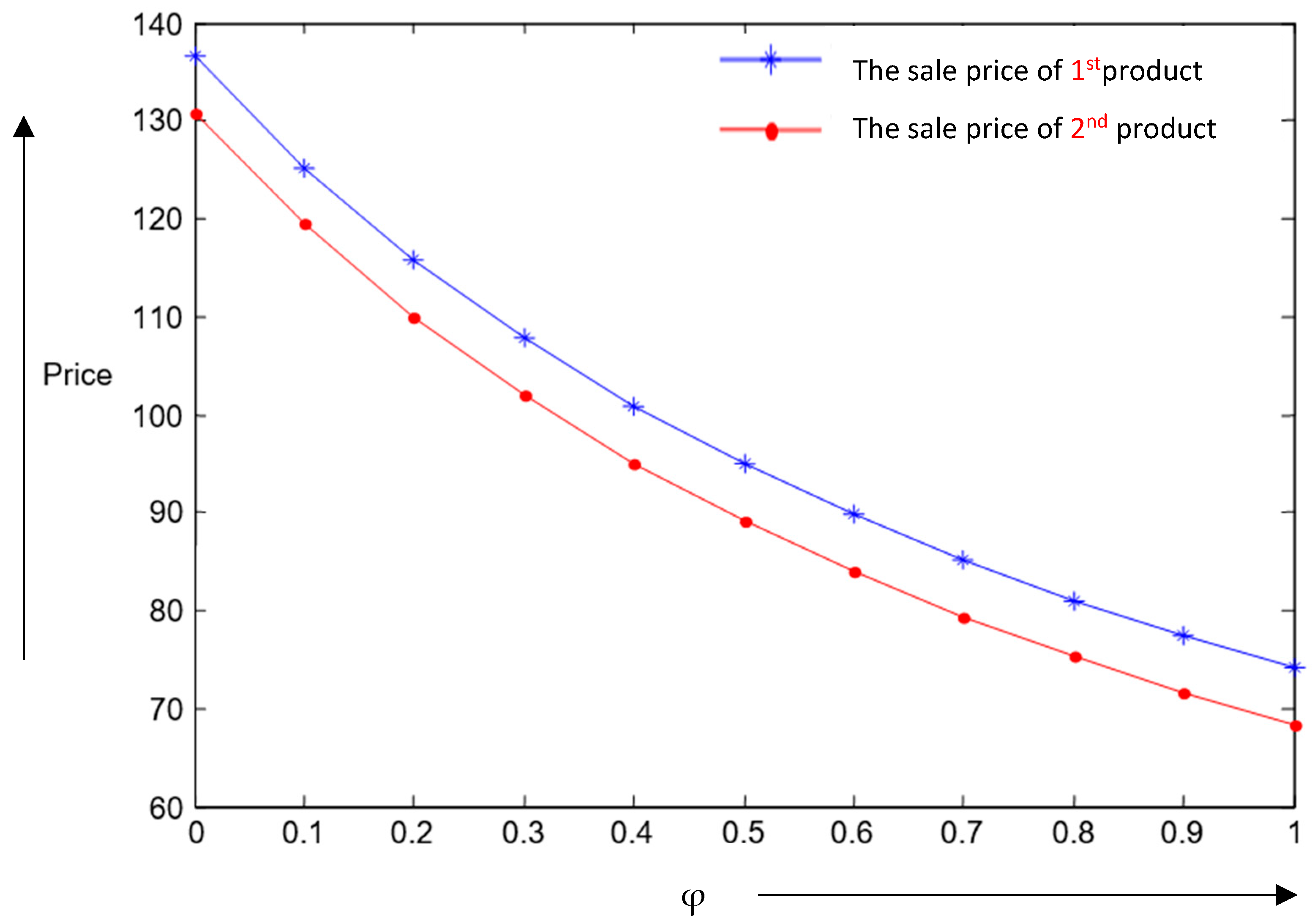
The values of all parameters are , , , , , , , and . By using Steps (1) to (5) of the proposed solution algorithm in Section 4.1, optimal values of , , , , and are obtained. These values with some variation of are depicted in the Table 2. ‘*’ demonstrates optimum results. Table 2 reveals the increasing value of gives decreasing values of , , , , and , but gives an increasing value of . More precisely, these changes on and are shown in Figure 3. Bold font indicates the optimum results.
5.2. Example 2: Non-Deteriorating Substitutable Products
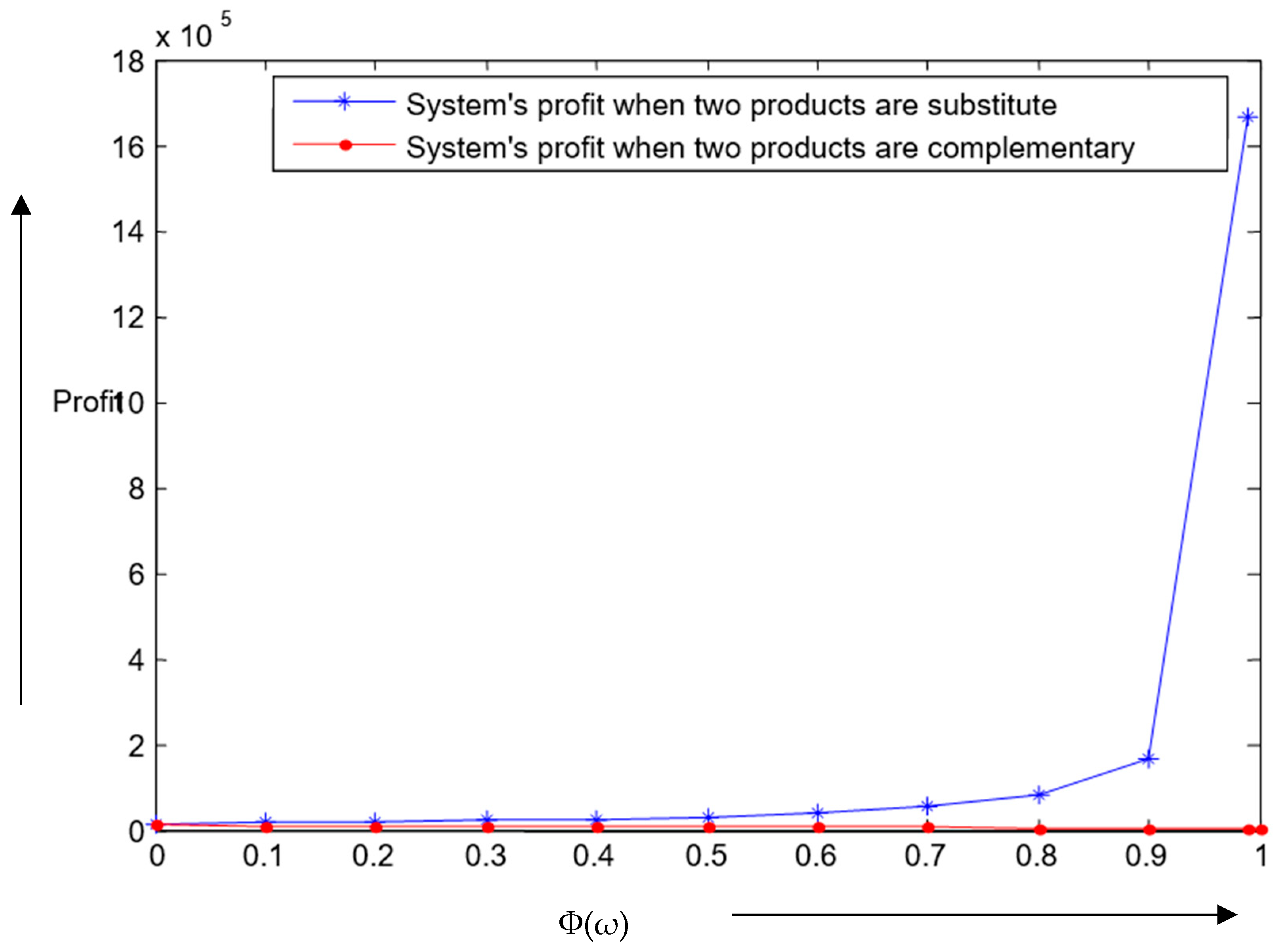
Values of parameters are , , , , , , , and . Steps (1) to (5) of the solution algorithm proposed in the Section 4.2 help to obtain optimum values of , , , , and for different values of d. Table 3 reveals that when increases, , , and decrease, but , , and increase. The changes on and are shown in Figure 4. Figure 5 reveals that the profit decreases whenever the degree of complementarity increases and vice-versa. Therefore, the retailer who intends to work on complementary products should select two products with a smaller degree of complementary to make more profit. But if he/she intends to work on substitutable products, he/she should select two products with a larger degree of substitutability.
5.3. Example 3: Deteriorating Complementary Products
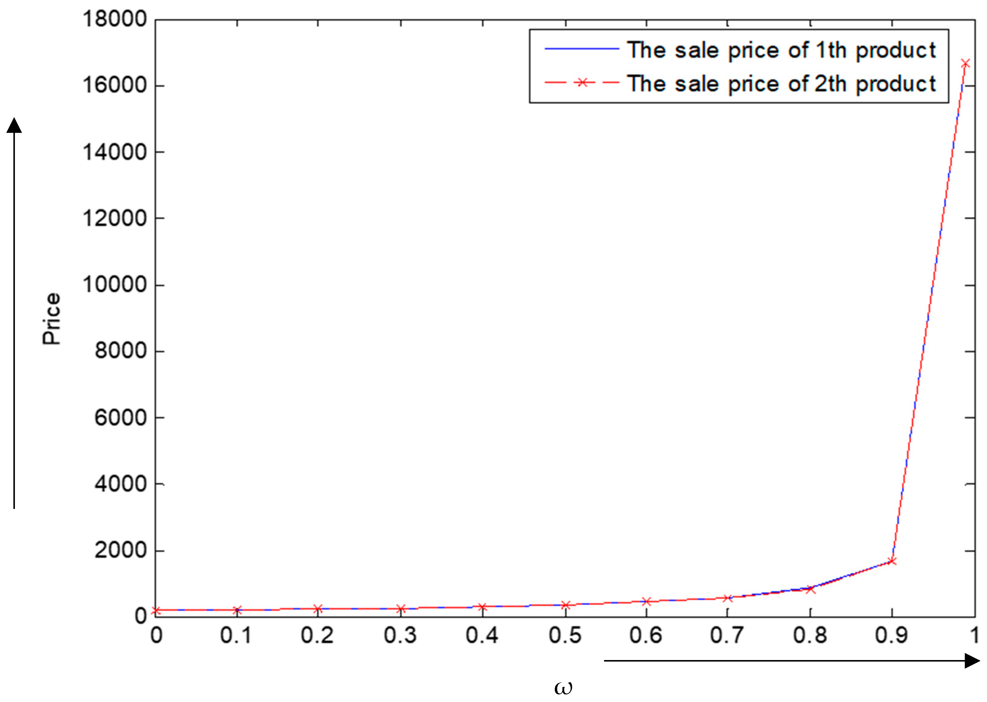
The values of parameters for this example are , , , , , , and . Using Steps (1) to (5) of the proposed solution algorithm in Section 4.3, the optimal values of , and are obtained. Table 4 shows that , , , and decrease when increases, but at that time, increases (similar to Section 5.1). The changes on and are shown in Figure 6 precisely.
5.4. Example 4: Deteriorating Substitutable Products
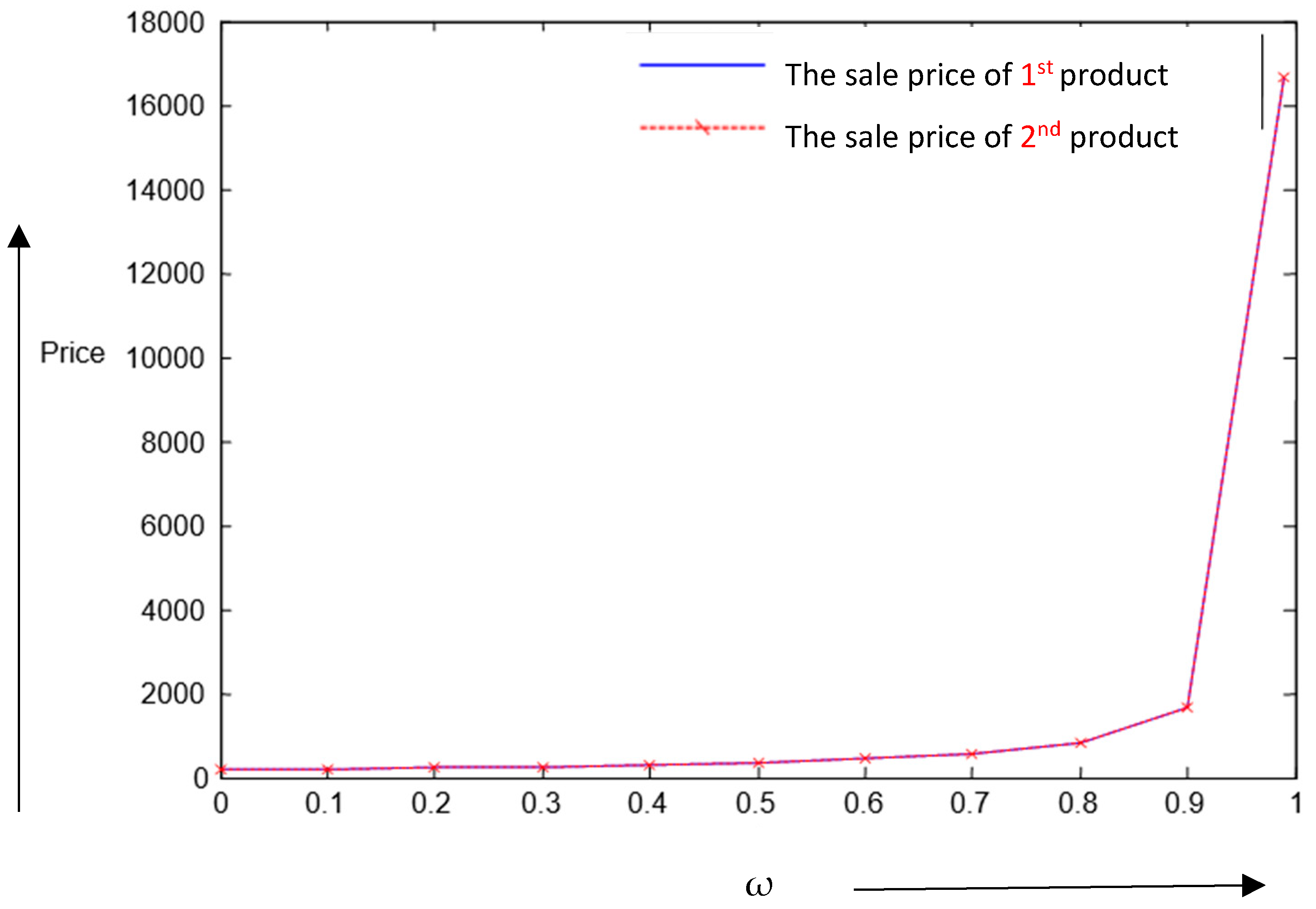
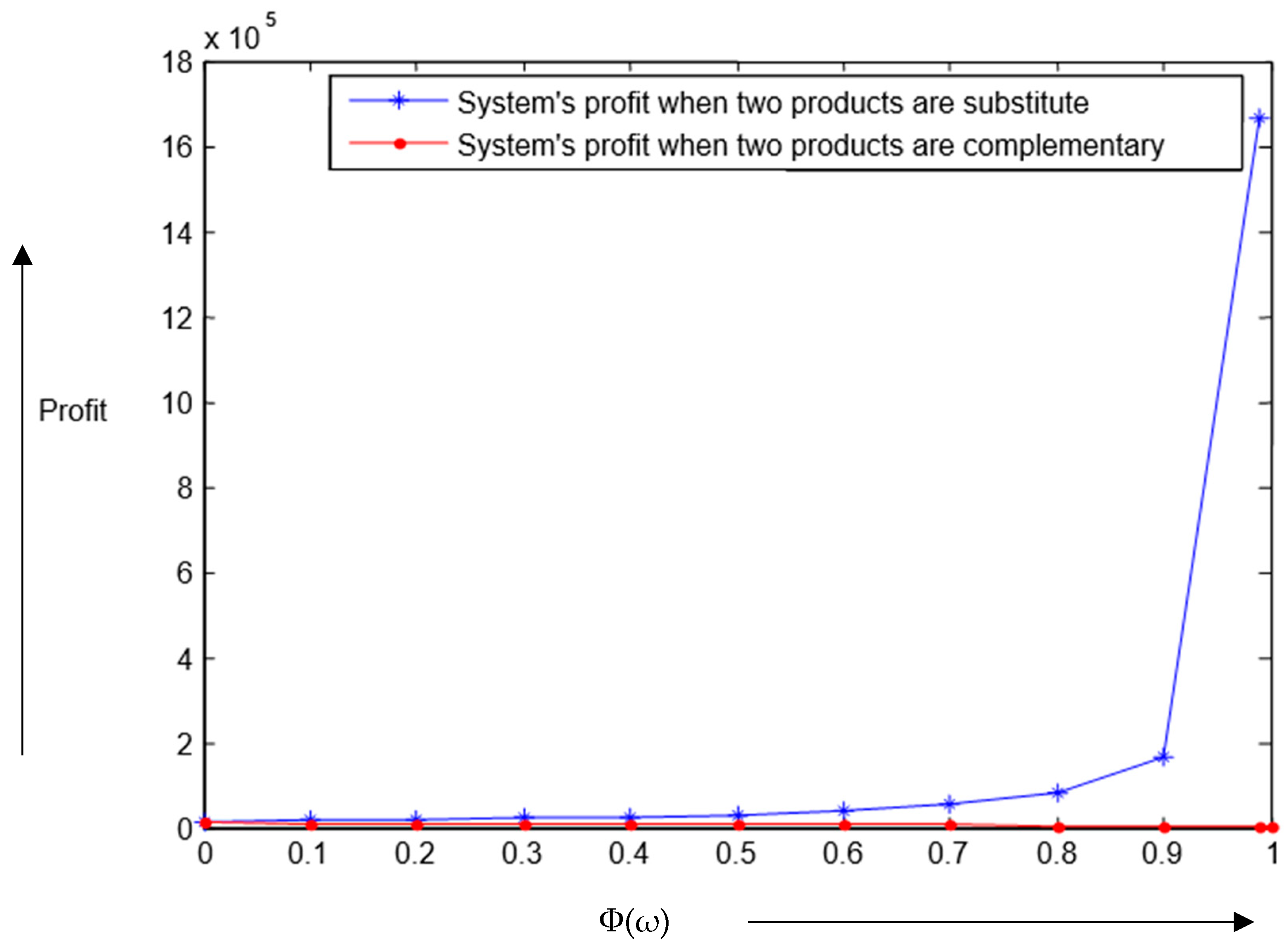
Fixed parametric values are , and . For different values of ω, one can use Steps (1) to (5) of proposed solution algorithm in Section 4.4. From the Table 5, it can be concluded that , , and decrease with increased values of ω, but , , and increase (similar Section 5.2). The changes on and are presented in the Figure 7. Figure 8 describes that the profit decreases when the complementarity degree increases, but profit increases while the degree of substitutability increases. As a result, the retailer who intends to work on complementary products should select two products with a smaller degree of complementary in order to make more profit. If he/she intends to work on substitutable products, he/she should select two products with a larger degree of substitutability.
Managerial insights
Numerical studies justify the theoretical implications of this research in each case separately. The degree of complementarity of a product has an inverse impact on the selling price, i.e., the increasing complementarity gives less profit. This implies that if one product is more dependent or complement to the other product, the selling of the one product is dependent upon the other product. In the case that one of the complementary products is not available at the right time, the chances to sale of the other product are smaller. To handle this situation, industry managers need to take more care of the inventory and safety stock of the complementary products.
For the case of substitutable products, the increasing rate of the degree of substitutability has a direct impact on the profit. This implies that if customers can get any similar substitutable product, the customer is satisfied with the service. The absence of the original product does not have any impact on the profit. This study suggests to industry managers that they should introduce similar types of alternative products to the shops or their centers such that they can survive facing losses from original products. It helps to keep the brand image of the industry as well as the retailer. The scenario is the same for the case of deteriorated substitutable and complementary products. Therefore, the industry needs to create their strategies carefully for complementary products rather than substitutable products.
6. Conclusions
Four pricing models for two types of products which may be complementary or substitutable and non-deteriorating or deteriorating were studied analytically as well as numerically. For all cases, it was observed that selling prices and lot sizes of both products as well as the average profit were decreased, and the period length was increased while the degree of complementarity was increased and vice versa. The selling prices and order quantities of both products as well as average profit were increased, and the cycle length was decreased with increased values of the degree of substitutability. This study concluded that sell of complementary products should be with some smaller degree of complementarity and substitutable products with bigger degree of substitutability in order to make more profit. The present model can help a manager to fix optimal selling prices, ordered quantities, and cycle length for different scenarios so that the joint profit is maximized. In the existing literature, some research articles are focused on substitutable and complementary products but none of them have investigated both inventory and pricing decisions of products simultaneously. Therefore, the present article is quite new compared to existing literature. Lead time is considered as zero in this study, but in reality it is not possible. This study can be extended with random lead time and backorder. The business can be spread through multiple number of retailers. Extra service facilities can be included within the study [45,46,47,48] for deteriorating products and non-zero random lead time. The quality improvement [49,50] and preservation technology [28,29] for deteriorating products can improve the study in a realistic way.
Author Contributions
Methodology, data curation, writing—original draft preparation, M.S.B.; formal analysis, conceptualization, visualization S.S.S.; investigation, S.S.S. and B.S.; resources, validation, supervision, project administration, A.A.T.; writing—review and editing, funding acquisition, B.S.
Funding
This research was supported by the Basic Science Research Program through the National Research Foundation of Korea (NRF) funded by the Ministry of Education, Science and Technology (Project Number: 2017R1D1A1B03033846).
Conflicts of Interest
The authors declare no conflict of interest.
Nomenclature
| Index | Description |
| 1, 2 | |
| Decision variables | |
| product ’s selling price ($/unit) | |
| order quantity of product (units) | |
| τ | time interval between two replenishments |
| Parameters | |
| market demand for product 1 (units) | |
| demand for product 2 (units) | |
| inventory level at time τ of product m | |
| ∝ | basic potential demand (units) |
| 𝛽 | self-price sensitivity |
| holding cost of product m ($/unit/unit time) | |
| purchasing cost of product m ($/unit) | |
| deterioration cost of product m ($/unit) | |
| deterioration rate of product 1 and product 2 | |
| degree of complementarity of two products, | |
| 𝜔 | degree of substitutability of two products, |
Appendix A
Proof of Theorem 1.
is strictly concave, if where
Now,
It has to show that the expression in Equation (A2) is negative. Therefore, the profit function is strictly concave if
holds; hence the proof.
Appendix B
Proof of Theorem 2.
is a concave whenever where
Thus, one can have
Then, it has to show that .
Hence, the profit function is concave if
holds. The proof is completed here.
Appendix C
Proof of Theorem 3.
is strictly concave if where
Now,
Now, it is needed to show that .
Therefore, the profit function is concave if
holds. The proof is completed here.
Appendix D
Proof of Theorem 4.
is a strictly concave function if holds.
where
Thus,
Then, it has to show that .
Then, the profit function is concave if
holds. The proof is completed here.
References
- Shocker, A.D.; Bayus, B.L.; Kim, N. Product complments and substitutes in the real world: The relevence of “other products”. J. Market. 2004, 68, 28–40. [Google Scholar] [CrossRef]
- Sarkar, M.; Lee, Y.H. Optimum pricing strategy for complementary products with stochastic reservation price in a supply chain model. J. Ind. Manag. Optim. 2017, 13, 1553–1586. [Google Scholar]
- Avgeropoulos, S.; Sammut-Bonnici, T.; McGee, J. Complementary products. Encycl. Manag. 2015, 12. [Google Scholar] [CrossRef]
- Sana, S.S. Price-sensitive demand for perishable items—An EOQ model. Appl. Math. Comput. 2011, 217, 6248–6259. [Google Scholar]
- Sarkar, B.; Saren, S.; Wee, H.M. An inventory model with variable demand, component cost and selling price for deteriorating items. Econ. Model. 2013, 30, 306–310. [Google Scholar] [CrossRef]
- Salvietti, L.; Smith, N.R.; Cárdenas-Barrón, L.E. A stochastic profit-maximising economic lot scheduling problem with price optimisation. Eur. J. Oper. Res. 2014, 8, 193–221. [Google Scholar] [CrossRef]
- Smith, N.R.; Robles, J.L.; Cárdenas-Barrón, L.E. Optimal pricing and production master planning in a multiperiod horizon considering capacity and inventory constraints. Math. Probl. Eng. 2009, 932676, 15. [Google Scholar] [CrossRef]
- Soon, W. A review of multi-product pricing models. Appl. Math. Comput. 2011, 217, 8149–8165. [Google Scholar] [CrossRef]
- Wei, J.; Zhao, J.; Li, Y. Pricing decisions for complementary products with firms’ different market powers. Eur. J. Oper. Res. 2013, 224, 507–519. [Google Scholar] [CrossRef]
- Dey, B.; Sarkar, B.; Sarkar, M.; Pareek, S. An integrated inventory model involving discrete setup cost reduction, variable safety factor, selling-price dependent demand, and investment. RAIRO-Oper. Res. 2019, 53, 39–57. [Google Scholar] [CrossRef]
- Mcgillivray, R.; Silver, E. Some concepts for inventory control under substitutable demand. Inf. Syst. Oper. Res. 1978, 16, 47–63. [Google Scholar] [CrossRef]
- Zhang, R.Q.; Kaku, I.; Xiao, Y.Y. Deterministic EOQ with partial backordering and correlated demand caused by cross-selling. Eur. J. Oper. Res. 2011, 210, 537–551. [Google Scholar] [CrossRef]
- Zhang, R.Q. An extension of partial backordering EOQ with correlated demand caused by cross-selling considering multiple minor items. Eur. J. Oper. Res. 2012, 220, 876–881. [Google Scholar] [CrossRef]
- Yue, X.; Mukhopadhyay, S.K.; Zhu, X. A Bertrand model of pricing of complementary goods under information asymmetry. J. Bus. Res. 2006, 59, 1182–1192. [Google Scholar] [CrossRef]
- Liu, L.; Yuan, X.M. Coordinated replenishments in inventory systems with correlated demands. Eur. J. Oper. Res. 2000, 123, 490–503. [Google Scholar] [CrossRef]
- Guchhait, R.; Sarkar, M.; Sarkar, B.; Pareek, S. Single-vendor multi-buyer game theoretic model under multi-factor dependent demand. Int. J. Inventory Res. 2017, 4, 303–332. [Google Scholar] [CrossRef]
- Shavandi, H.; Mahlooji, H.; Nosratian, N.E. A constrained multi-product pricing and inventory control problem. Appl. Soft Comput. 2012, 12, 2454–2461. [Google Scholar] [CrossRef]
- Abad, P.L. Optimal pricing and lot-sizing under conditions of perishability, finite production and partial backordering and lost sale. Eur. J. Oper. Res. 2003, 144, 677–685. [Google Scholar] [CrossRef]
- Balkhi, Z.T.; Benkherouf, L. On an inventory model for deteriorating items with stock dependent and time-varying demand rates. Comput. Oper. Res. 2004, 31, 223–240. [Google Scholar] [CrossRef]
- Anjos, M.F.; Cheng, R.C.; Currie, C.S. Optimal pricing policies for perishable products. Eur. J. Oper. Res. 2005, 166, 246–254. [Google Scholar] [CrossRef] [Green Version]
- Dye, C.Y. Joint pricing and ordering policy for a deteriorating inventory with partial backlogging. Omega 2007, 35, 184–189. [Google Scholar] [CrossRef]
- Panda, S.; Saha, S.; Basu, M. An EOQ model for perishable products with discounted selling price and stock dependent demand. Cent. Eur. J. Oper. Res. 2009, 17, 31. [Google Scholar] [CrossRef]
- Pang, Z. Optimal dynamic pricing and inventory control with stock deterioration and partial backordering. Oper. Res. Lett. 2011, 39, 375–379. [Google Scholar] [CrossRef]
- Sarkar, B.; Majumder, A.; Sarkar, M.; Dey, B.K.; Roy, G. Two-echelon supply chain model with manufacturing quality improvement and setup cost reduction. J. Ind. Manag. Optim. 2017, 13, 1085–1104. [Google Scholar] [CrossRef] [Green Version]
- Sarkar, B.; Saren, S. Partial trade-credit policy of retailer with exponentially deteriorating items. Int. J. Appl. Comput. Math. 2015, 1, 343–368. [Google Scholar] [CrossRef]
- Sett, B.K.; Sarkar, B.; Sarkar, B.; Yun, W.Y. Optimal replenishment policy with variable deterioration for fixed lifetime products. Sci. Iran. 2016, 23, 2318–2329. [Google Scholar] [Green Version]
- Sarkar, B.; Sett, B.K.; Roy, G.; Goswami, A. Flexible setup cost and deterioration of products in a supply chain model. Int. J. Appl. Comput. Math. 2016, 2, 25–40. [Google Scholar] [CrossRef]
- Sarkar, B.; Mandal, B.; Sarkar, S. Preservation of deteriorating seasonal products with stock-dependent consumption rate and shortages. J. Ind. Manag. Optim. 2017, 13, 187–206. [Google Scholar] [CrossRef] [Green Version]
- Ullah, M.; Sarkar, B.; Asghar, I. Effects of preservation technology investment on waste generation in a two-echelon supply chain model. Mathematics 2019, 7, 20. [Google Scholar] [CrossRef]
- Iqbal, M.W.; Sarkar, B. Recycling of lifetime dependent deteriorated products through different supply chains. RAIRO-Operat. Res. 2019, 53, 129–156. [Google Scholar] [CrossRef]
- Dey, B.K.; Sarkar, B.; Pareek, S. A two-echelon supply chain management with setup time and cost reduction, quality improvement and variable production rate. Mathematics 2019, 7, 25. [Google Scholar] [CrossRef]
- Gürler, Ü.; Yılmaz, A. Inventory and coordination issues with two substitutable products. Appl. Math. Model. 2010, 34, 539–551. [Google Scholar] [CrossRef] [Green Version]
- Kim, S.W.; Bell, P.C. Optimal pricing and production decisions in the presence of symmetrical and asymmetrical substitution. Omega 2011, 39, 528–538. [Google Scholar] [CrossRef]
- Stavrulaki, E. Inventory decisions for substitutable products with stock-dependent demand. Int. J. Prod. Econ. 2011, 129, 65–78. [Google Scholar] [CrossRef]
- Karakul, M.; Chan, L.M.A. Analytical and managerial implications of integrating product substitutability in the joint pricing and procurement problem. Eur. J. Oper. Res. 2008, 190, 179–204. [Google Scholar] [CrossRef]
- Karakul, M.; Chan, L.M.A. Joint pricing and procurement of substitutable products with random demands–a technical note. Eur. J. Oper. Res. 2010, 201, 324–328. [Google Scholar] [CrossRef]
- Birge, J.R.; Drogosz, J.; Duenyas, I. Setting single-period optimal capacity levels and prices for substitutable products. Int. J. Flex. Manuf. Syst. 1998, 10, 407–430. [Google Scholar] [CrossRef]
- Netessine, S.; Dobson, G.; Shumsky, R.A. Flexible service capacity: Optimal investment and the impact of demand correlation. Oper. Res. 2002, 50, 375–388. [Google Scholar] [CrossRef]
- Parlar, M.; Goyal, S. Optimal ordering decisions for two substitutable products with stochastic demands. Opsearch 1984, 21, 1–15. [Google Scholar]
- Pasternack, B.A.; Drezner, Z. Optimal inventory policies for substitutable commodities with stochastic demand. Nav. Res. Logist. 1991, 38, 221–240. [Google Scholar] [CrossRef]
- Tang, C.S.; Yin, R. Joint ordering and pricing strategies for managing substitutable products. Prod. Oper. Manag. 2007, 16, 138–153. [Google Scholar] [CrossRef]
- Xia, Y. Competitive strategies and market segmentation for suppliers with substitutable products. Eur. J. Oper. Res. 2011, 210, 194–203. [Google Scholar] [CrossRef]
- Netessine, S.; Rudi, N. Centralized and competitive inventory models with demand substitution. Oper. Res. 2003, 51, 329–335. [Google Scholar] [CrossRef]
- Gupta, S.; Loulou, R.J.M.S. Process innovation, product differentiation, and channel structure: Strategic incentives in a duopoly. Market. Sci. 1998, 17, 301–316. [Google Scholar] [CrossRef]
- Sarkar, M.; Guchhait, R.; Sarkar, B. Modelling for service solution of a closed-loop supply chain with the presence of third party logistics. In Advances in Production Management Systems. Production Management for Data-Driven, Intelligent, Collaborative, and Sustainable Manufacturing; APMS 2018; IFIP Advances in Information and Communication Technology; Springer: Cham, Switzerland, 2018; Volume 535, pp. 320–327. [Google Scholar]
- Khanna, A.; Kishore, A.; Sarkar, B.; Jaggi, C. Supply chain with customer-based two-level credit policies under an imperfect quality environment. Mathematics 2018, 6, 35. [Google Scholar] [CrossRef]
- Guchhait, R.; Pareek, S.; Sarkar, B. Application of distribution-free approach in integrated and dual-channel supply chain under buyback contract. In Handbook of Research on Promoting Business Process Improvement Through Inventory Control Techniques; IGI Global: Hershey, PA, USA, 2018; pp. 388–426. [Google Scholar]
- Guchhait, R.; Dey, B.K.; Bhuniya, S.; Mandal, B.; Bachar, R.; Chauduri, K.S.; Wee, H.M.; Sarkar, B. Investment for process quality improvement and setup cost reduction in an imperfect production process with warranty policy and shortages. RAIRO-Oper. Res. 2019. [Google Scholar] [CrossRef]
- Shin, D.; Guchhait, R.; Sarkar, B.; Mittal, M. Controllable lead time, service level constraint, and transportation discounts in a continuous review inventory model. RAIRO-Oper. Res. 2016, 50, 921–934. [Google Scholar] [CrossRef]
- Majumder, A.; Guchhait, R.; Sarkar, B. Manufacturing quality improvement and setup cost reduction in a vendor-buyer supply chain model. Eur. J. Ind. Eng. 2017, 11, 588–612. [Google Scholar] [CrossRef]
Figure 1.
Inventory level of two products (complementary or substitutable) without shortage under EOQ policy.
Figure 1.
Inventory level of two products (complementary or substitutable) without shortage under EOQ policy.

Figure 2.
Inventory level of two deteriorating products (complementary or substitutable) without shortage under EOQ policy.
Figure 2.
Inventory level of two deteriorating products (complementary or substitutable) without shortage under EOQ policy.

Figure 3.
Changes of the complementarity degree upon selling prices.
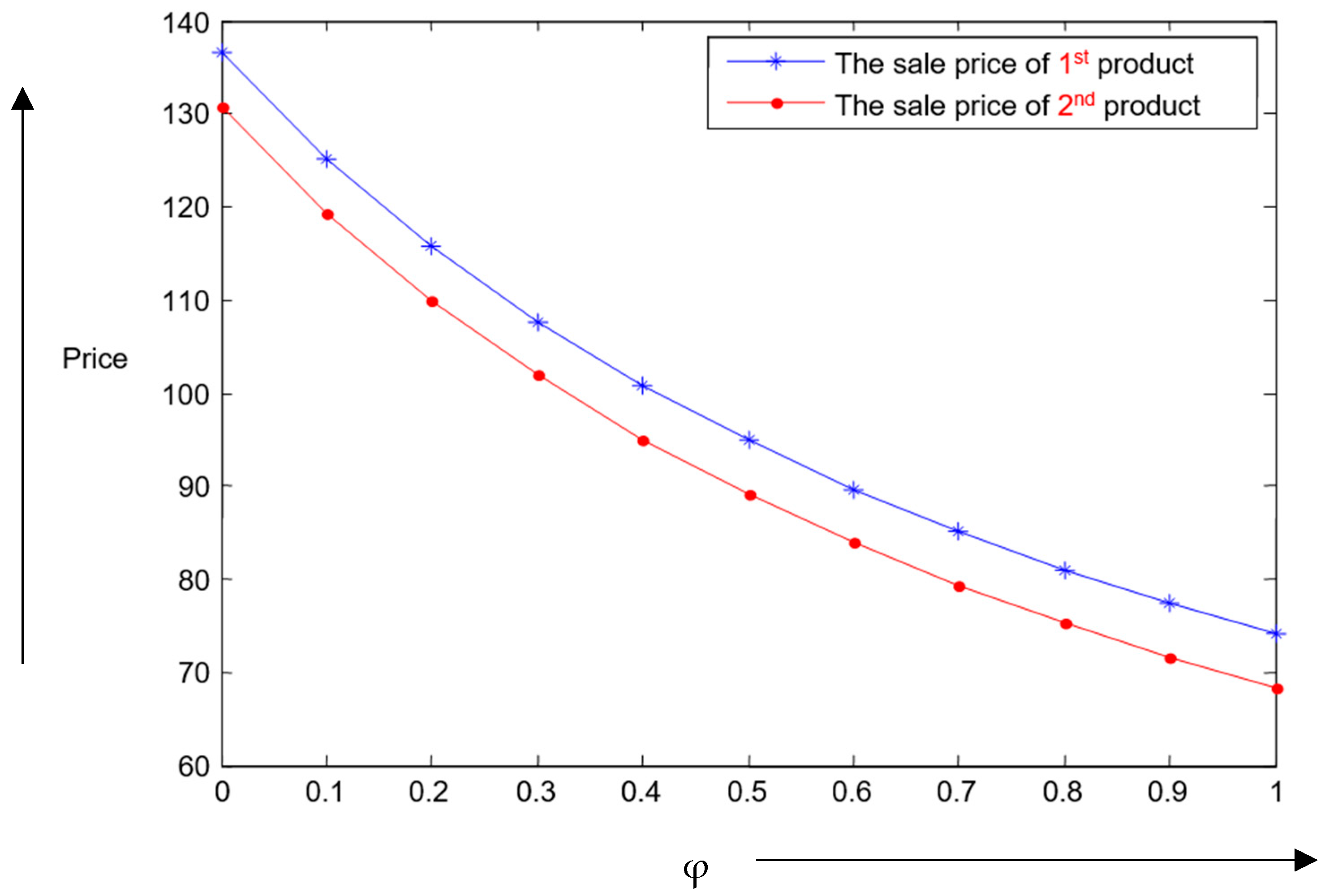
Figure 4.
Changes in the degree of substitutability upon selling prices.

Figure 5.
Effects of the changes of complementarity and substitutability degrees on profits.

Figure 6.
Effects of changes of complementarity degree on selling prices of deteriorating products.

Figure 7.
Changes in the degree of substitutability upon selling prices of deteriorating products.

Figure 8.
Changes of the complementarily and substitutability degrees upon profits of deteriorating products.
Figure 8.
Changes of the complementarily and substitutability degrees upon profits of deteriorating products.

Table 1.
Author’s contributions table.
| Author(s) | Inventory | Pricing | Deterioration | Complementary Products | Substitutable Products |
|---|---|---|---|---|---|
| Sarkar and Lee [2] | √ | √ | |||
| Sana [4] | √ | √ | |||
| Smith et al. [7] | √ | √ | |||
| Wei at al. [9] | √ | √ | |||
| Mcgillivray and Silver [11] | √ | √ | |||
| Yue et al. [14] | √ | √ | |||
| Balkhi and Benkherouf [19] | √ | √ | |||
| Dye [21] | √ | √ | √ | ||
| Karakul and Chan [35] | √ | √ | √ | ||
| Tang and Yin [41] | √ | √ | √ | ||
| This study | √ | √ | √ | √ | √ |
Table 2.
Optimum results for some variations of φ.
| φ | Concavity | τ | |||||
|---|---|---|---|---|---|---|---|
| 0 | True | 93.3221 | 274.9832 | 199.9916 | −932.5924 | 1866.8 | 1247.6 |
| True | 1.0290 * | 136.5438 * | 130.7719 * | 46.7087 * | 49.0849 * | 10621 * | |
| False | −1.0180 | - | - | - | - | - | |
| 0.1 | True | 85.9137 | 252.5069 | 183.0716 | −715.2833 | 1432.3 | 944.4092 |
| True | 1.0327 * | 125.1854 * | 119.4109 * | 46.6255 * | 48.7723 * | 8548.6 * | |
| False | −1.0229 | - | - | - | - | - | |
| 0.2 | True | 79.5269 | 233.4570 | 168.8118 | −547.7619 | 1097.4 | 715.6247 |
| True | 1.0362 * | 115.7210 * | 109.9438 * | 46.4588 * | 48.1415 * | 7752.7 * | |
| False | −1.0229 | - | - | - | - | - | |
| 0.3 | True | 73.9641 | 217.1000 | 156.6269 | -416.8036 | 835.5901 | 539.8298 |
| True | 1.0398 * | 107.7135 * | 101.9337 * | 46.4588 * | 48.1415 * | 7752.7 * | |
| False | −1.0253 | - | - | - | - | - | |
| 0.4 | True | 69.0754 | 202.8988 | 146.0923 | −313.2069 | 628.5371 | 402.6596 |
| True | 1.0433 * | 100.8607 * | 95.0682 * | 46.3753 * | 47.5031 * | 6481.3 * | |
| False | −1.0278 | - | - | - | - | - | |
| 0.5 | True | 64.7452 | 190.4512 | 136.8923 | −230.4240 | 463.1133 | 294.2216 |
| True | 1.0470 * | 94.9038 * | 89.1186 * | 46.2917 * | 47.5031 * | 6481.3 * | |
| False | −1.0303 | - | - | - | - | - | |
| 0.6 | True | 60.8831 | 179.4496 | 128.7873 | −163.7025 | 329.8139 | 207.5357 |
| True | 1.0606 * | 89.7010 * | 83.9130 * | 46.2079 * | 47.1809 * | 5965.9 * | |
| False | −1.0328 | - | - | - | - | - | |
| 0.7 | True | 57.4169 | 169.6547 | 121.5921 | −109.5329 | 221.6201 | 137.5717 |
| True | 1.0644 * | 85.1110 * | 79.3202 * | 46.0401 * | 46.5305 * | 5108.5 * | |
| False | −1.0353 | - | - | - | - | - | |
| 0.8 | True | 54.2887 | 160.8775 | 115.1610 | −65.2832 | 133.2681 | 80.6367 |
| True | 1.0581 * | 81.0316 * | 75.2380 * | 46.0401 * | 46.5305 * | 5108.5 * | |
| False | −1.0379 | - | - | - | - | - | |
| 0.9 | True | 51.4514 | 152.9666 | 109.3780 | −28.9524 | 60.7553 | 33.9747 |
| True | 1.0619 * | 77.3824 * | 71.5859 * | 45.9560 * | 46.2022 * | 4748.4 * | |
| False | −1.0404 | - | - | - | - | - | |
| 1.0 | True | 48.8661 | 145.7992 | 104.1496 | 1.0005 | 1.0005 | −4.5010 |
| True | 1.0658 * | 74.0987 * | 68.2993 * | 45.8717 * | 45.8717 * | 4424.9 * | |
| False | −1.0430 | - | - | - | - | - |
“-“ means infeasible result; “*” means optimum solution.
Table 3.
Optimum results for some variations of ω.
| Concavity | τ | ||||||
|---|---|---|---|---|---|---|---|
| 0 | True | 149.7187 | 342.6002 | 322.8854 | −416.2286 | 469.2757 | 56.4733 |
| True | 1.2292 * | 175.5495 | 174.3959 * | 58.1837 * | 58.6091 * | 14,799 * | |
| False | −1.2170 | - | - | - | - | - | |
| 0.1 | True | 380.5094 | 358.6400 | −566.5791 | 638.3149 | 77.4294 | |
| True | 194.0644 * | 192.9112 * | 58.3172 * | 58.7838 * | 16,647 * | ||
| False | −1.2170 | - | - | - | - | - | |
| 0.2 | True | 188.4626 | 427.8537 | 403.2959 | −783.6958 | 882.4670 | 107.5095 |
| True | 1.2228 * | 217.2090 * | 216.0561 * | 58.4503 * | 58.9578 * | 18,957 * | |
| False | −1.2149 | - | - | - | - | - | |
| 0.3 | True | 216.0547 | 488.6568 | 460.6500 | −1110.2 | 1249.7 | 152.5353 |
| True | 246.9673 * | 245.8149 * | 58.5830 * | 59.1312 * | 21,929 * | ||
| False | −1.2107 | - | - | - | - | - | |
| 0.4 | True | 252.7386 | 569.6088 | 537.0164 | −1627.8 | 1831.9 | 223.6789 |
| True | 1.2165 * | 286.6464 * | 285.4943 * | 58.7153 * | 59.3039 * | 25,894 * | |
| False | −1.2107 | - | - | - | - | - | |
| 0.5 | True | 303.8947 | 682.7149 | 643.7281 | −2508.7 | 2822.8 | 344.5513 |
| True | 1.2134 * | 342.1984 * | 341.0467 * | 58.8472 * | 59.4761 * | 31,445 * | |
| False | −1.2086 | - | - | - | - | - | |
| 0.6 | True | 380.1918 | 851.8825 | 803.3585 | −4167.0 | 4688.3 | 572.1289 |
| True | 1.2103 * | 425.5283 * | 424.3770 * | 58.9787 * | 59.6475 * | 39,774 * | |
| False | −1.2065 | - | - | - | - | - | |
| 0.7 | True | 506.2033 | 1132.5 | 1068.3 | −7808.6 | 8784.9 | 1073.6 |
| True | 1.2073 * | 564.4137 * | 563.2628 * | 59.1098 * | 59.8184 * | 53,659 * | |
| False | −1.2044 | - | - | - | - | - | |
| 0.8 | True | 753.9936 | 1689.1 | 1593.8 | −18,250 | 20,531 | 2525.4 |
| True | 1.2043 * | 842.1881 * | 841.0376 * | 59.2405 * | 59.9887 * | 81,433 * | |
| False | −1.2013 | - | - | - | - | - | |
| 0.9 | True | 1465.2 | 3322.5 | 3138.4 | −72,373 | 81,420 | 10,300 |
| True | 1.2013 * | 1675.5 * | 1674.4 * | 59.3708 * | 60.1583 * | 164,760 * | |
| False | - | - | - | - | - | - | |
| 1.0 | Undefined | 22659 | ∞ | ∞ | ∞ | ∞ | Undefined |
| Undefined | 1.1983 | −∞ | ∞ | ∞ | −∞ | Undefined | |
| Undefined | −1.1982 | −∞ | ∞ | −∞ | ∞ | Undefined |
“-“ means infeasible result; “*” means optimum solution.
Table 4.
Optimum results for some variations of φ (deterioration case).
| φ | Concavity | τ | |||||
|---|---|---|---|---|---|---|---|
| 0 | True | 91.7921 | 274.9829 | 199.9914 | −1503.0 | 3008.7 | 1247.6 |
| True | 1.0208 * | 136.5567 * | 130.7784 * | 46.5584 * | 48.9299 * | 10,618 * | |
| False | −1.0096 | - | - | - | - | - | |
| 0.1 | True | 84.5050 | 252.5065 | 183.0715 | −1105.7 | 2214.1 | 944.3665 |
| True | 1.0242 * | 125.1983 * | 119.4174 * | 46.4762 * | 48.6187 * | 9486.7 * | |
| False | −1.0120 | - | - | - | - | - | |
| 0.2 | True | 78.2230 | 233.4567 | 168.8117 | −817.1057 | 1637.0 | 715.5786 |
| True | 1.0277 * | 115.7340 * | 109.9503 * | 46.3938 * | 48.3057 * | 8545.1 * | |
| False | −1.0144 | - | - | - | - | - | |
| 0.3 | True | 72.7513 | 217.0996 | 156.6267 | −602.9090 | 1208.7 | 539.7803 |
| True | 1.0313 * | 107.7265 * | 101.9402 * | 46.3114 * | 47.9908 * | 7749.2 * | |
| False | −1.0168 | - | - | - | - | - | |
| 0.4 | True | 67.9427 | 202.8984 | 146.0921 | −441.0527 | 885.1454 | 402.6065 |
| True | 1.0348 * | 100.8638 * | 95.0748 * | 46.2288 * | 47.6741 * | 7067.7 * | |
| False | −1.0193 | - | - | - | - | - | |
| 0.5 | True | 63.6836 | 190.4508 | 136.8921 | −316.9006 | 636.9689 | 294.1649 |
| True | 1.0384 * | 94.9169 * | 89.1251 * | 46.1462 * | 47.3553 * | 6477.9 * | |
| False | −1.0218 | - | - | - | - | - | |
| 0.6 | True | 59.8847 | 179.4492 | 128.7871 | −220.4678 | 444.2343 | 207.4755 |
| True | 1.0421 * | 89.7142 * | 83.9196 * | 46.0634 * | 47.0346 * | 5962.4 * | |
| False | −1.0243 | - | - | - | - | - | |
| 0.7 | True | 56.4753 | 169.6543 | 121.5918 | −144.7758 | 292.9846 | 137.5079 |
| True | 1.0458 * | 85.1242 * | 79.3268 * | 45.9805 * | 46.7119 * | 5508.2 * | |
| False | −1.0268 | - | - | - | - | - | |
| 0.8 | True | 53.3984 | 160.8770 | 115.1607 | −84.8435 | 173.2576 | 80.5692 |
| True | 1.0495 * | 81.0449 * | 75.2447 * | 45.8975 * | 46.3871 * | 5105.1 * | |
| False | −1.0293 | - | - | - | - | - | |
| 0.9 | True | 50.6076 | 152.9660 | 109.3778 | −37.0492 | 77.8092 | 33.9034 |
| True | 1.0533 * | 77.3957 * | 71.5926 * | 45.8144 * | 46.0602 * | 4745.0 * | |
| False | −1.0318 | - | - | - | - | - | |
| 1.0 | True | 48.0647 | 145.7986 | 104.1493 | 1.2845 | 1.2845 | −4.5761 |
| True | 1.0571 * | 74.1121 * | 68.3060 * | 45.7312 * | 45.7312 * | 4421.4 * | |
| False | −1.0344 | - | - | - | - | - |
“-“ means infeasible result; “*” means optimum solution.
Table 5.
Optimum results for some variations of ω (deterioration case).
| ω | Concavity | τ | |||||
|---|---|---|---|---|---|---|---|
| 0 | True | 147.4584 | 342.6379 | 322.8369 | −940.472 | 1060.9 | 56.9563 |
| True | 1.2199 * | 175.5604 * | 174.4049 * | 58.0953 * | 58.5208 * | 14,795 * | |
| False | −1.2099 | - | - | - | - | - | |
| 0.1 | True | 164.4331 | 380.5500 | 358.5848 | −1423.5 | 1604.6 | 78.1010 |
| True | 1.2167 * | 194.0753 * | 192.9202 * | 58.2279 * | 58.6945 * | 16,643 * | |
| False | −1.2078 | - | - | - | - | - | |
| 0.2 | True | 185.6144 | 427.8978 | 403.2320 | −2254.3 | 2539.8 | 108.4521 |
| True | 1.2136 * | 217.2198 * | 216.0651 * | 58.3600 * | 58.8676 * | 18,954 * | |
| False | −1.2057 | - | - | - | - | - | |
| 0.3 | True | 212.7872 | 488.7046 | 460.5742 | −3816.6 | 4298.5 | 153.8840 |
| True | 1.2104 * | 246.9782 * | 245.8238 * | 56.4918 * | 59.0400 * | 21,926 * | |
| False | −1.2036 | - | - | - | - | - | |
| 0.4 | True | 248.9126 | 569.6604 | 536.9240 | −7146.8 | 8047.2 | 225.6693 |
| True | 1.2073 * | 286.6572 * | 285.5032 * | 58.6231 * | 59.2118 * | 25,890 * | |
| False | −1.2015 | - | - | - | - | - | |
| 0.5 | True | 299.2879 | 682.7698 | 643.6106 | −15,703 | 17,678 | 347.6315 |
| True | 1.2043 * | 342.2092 * | 341.0556 * | 58.7540 * | 59.3829 * | 31441 * | |
| False | −1.1994 | - | - | - | - | - | |
| 0.6 | True | 374.4167 | 851.9377 | 803.1996 | −45,423 | 51134 | 577.2581 |
| True | 1.2012 * | 425.5390 * | 424.3859 * | 58.8845 * | 59.5534 * | 39,770 * | |
| False | −1.1974 | - | - | - | - | - | |
| 0.7 | True | 498.4871 | 1132.6 | 1068.0 | −224,880 | 253,130 | 1083.2 |
“-“ means infeasible result; “*” means optimum solution.
© 2019 by the authors. Licensee MDPI, Basel, Switzerland. This article is an open access article distributed under the terms and conditions of the Creative Commons Attribution (CC BY) license (http://creativecommons.org/licenses/by/4.0/).
Share and Cite
MDPI and ACS Style
Taleizadeh, A.A.; Babaei, M.S.; Sana, S.S.; Sarkar, B. Pricing Decision within an Inventory Model for Complementary and Substitutable Products. Mathematics 2019, 7, 568. https://doi.org/10.3390/math7070568
AMA Style
Taleizadeh AA, Babaei MS, Sana SS, Sarkar B. Pricing Decision within an Inventory Model for Complementary and Substitutable Products. Mathematics. 2019; 7(7):568. https://doi.org/10.3390/math7070568
Chicago/Turabian StyleTaleizadeh, Ata Allah, Masoumeh Sadat Babaei, Shib Sankar Sana, and Biswajit Sarkar. 2019. "Pricing Decision within an Inventory Model for Complementary and Substitutable Products" Mathematics 7, no. 7: 568. https://doi.org/10.3390/math7070568
Note that from the first issue of 2016, this journal uses article numbers instead of page numbers. See further details here.