


Abstract
Symmetric quantum calculus offers a dynamic framework for investigating the various classes of functions. However, the symmetric quantum operators become inconclusive at certain points. To overcome the limitations of existing calculi, operators over finite intervals have been extensively explored. To develop a more general and applicable setup, we introduce the symmetric quantum derivative and integral operators governed by an arbitrary point. Furthermore, we discuss structural properties of the newly developed operators and special cases to relate to the existing literature. Then, by applying the concepts of general symmetric quantum operators, convexity, Lipschitzian property, and Korkine’s identity, we derive a new set of inequalities, including Hermite–Hadamard, Ostrowski, Hólder, Minkowski, and Gruss-type inequalities, respectively. The proposed inequalities are useful to derive the bounds of generalized symmetric quantum integrals. Furthermore, the newly developed operators can be applied to study the impulsive difference equations and their dynamics. Additionally, a feed-forward ANN model is established to approximate the analytic expressions involved in inequalities and to observe the consistency of integral bounds. The results of the ANN analysis suggest a significant agreement between analytical solutions and approximations. Lastly, we focus on an applicable analysis of our derived results. The generic nature of operators will lead to new developments in quantum calculus. The hybrid approach evolved in this study will bring new applicable insights to the mathematical analysis.
Keywords:
symmetric quantum operators; convex function; Hermite–Hadamard; Hölder; Grüss; inequalities; artificial neural network MSC:
39A13; 26D15; 26A51; 39A70
1. Motivation and Problem Background
The fundamental concepts of calculus are defined over a uniform grid, and they become inconclusive in a few scenarios, particularly when working on systems that have singularities and multi-scale behavior. In the following perspective, the dynamics studied over non-uniform grids play a critical role. The -formation of classical concepts by replacing a limiting approach with difference quotients depending upon a parameter is known as quantum calculus. The early contributions in discrete structures were due to Euler and Gauss, as they proved -series, -identities, -factorials, and hypergeometric series. However, systematically, it was initiated by Jackson in 1908. He presented the idea of -derivative and its inverse operator over a non-uniform grid over in [1,2]. These operators are equally useful for analyzing those functions which are not differentiable and integrable in the classical sense. Focusing on these operators, a range of advancements have been made in special functions to generalize the various fundamental polynomials using -calculus and mathematical inequalities. For deep investigation, see [3]. One can notice that the -derivative of several functions cannot be calculated at the origin. To fill this gap, Tariboon and Ntoyas [4] extended the -concepts over fine intervals using the left endpoint and enabled them to apply to impulsive difference equations, as Jackson operators cannot be applied if the impulse lies between and , while the right operators were discussed in [5].
The symmetric derivative was developed to analyze functions whose classical derivative at some points does not exist. They are extensively studied and generalized using different approaches. The symmetric quantum derivative and inverse operators were defined using and in [3]. Motivated by [4], Bilal et al. [6] developed the left-symmetric quantum calculus and derived the fundamental inequalities. Following these developments, authors [7] presented the right-symmetric quantum calculus and discussed the key properties of this calculus and established diverse inequalities under convexity assumptions within this framework.
To move further, first we recall the left-symmetric quantum derivative and definite integral. In 2024, Bilal et al. [6] delivered the concepts related to finite symmetric quantum operators.
Definition 1
([6]). Let be a function and . Then
And , if the limit exists. If , then .
The definite symmetric antiderivative operators is given as
Definition 2
([6]). Let be a function and . Then
Another kind of symmetric operators are listed in [7].
Definition 3
([7]). Let be a function and . Then
Furthermore, , if the limit exists. If , then .
Definition 4
([7]). Let be a function and . Then
Convex functions are useful to prove the discrete and continuous variants of classical inequalities. In recent years, the contributions of convexity and discrete dynamics are exceptional. One of the leading discrete structures is quantum calculus and its generalizations. The quantum-based Hermite–Hadamard inequalities and their improvements are studied in [8,9,10,11]. The left and right estimations of the Hadamard inequality and error analytical inequalities within the q-framework are discussed in [12,13,14,15]. Furthermore, Ref. [16] discussed the symmetric quantum Ostrowski-type inequalities. After the evolution of the complete structure of symmetric operators, Liu et al. [17] established the refined Hadamard inequalities and unified error approximations. For a complete investigation, we refer to [18,19].
Theorem 1
([7]). Let be a convex function and . Then
It is already revealed that finite quantum calculi were defined through the left and right endpoints of the interval. An obvious question arises: why can the other points of the interval not be used, except for the endpoints? To seek out this problem, recently, authors [20] defined the quantum operators using an arbitrary point of the domain except the midpoint of the interval. The general derivative operator is stated as
Definition 5
([20]). Let and be a function. Then generalized -difference quotient of V at is stated as
where . For , we define .
Remark 1.
Definition 6
([20]). Suppose that and the generalized definite -integral of real valued function V defined J is defined as
if , then we will use for and if , then we will express for .
Remark 2.
We deduce the following representation from Definition 6.
and
Remark 3.
Therefore, we can write
or
Artificial neural network (ANN) modeling is an effective tool following the principle of the human brain. The mechanism of ANN consists of collecting data in terms of neurons and manipulating them to transfer to hidden layers for further computations. Finally, it leads to the final outcome. During manipulations of information, it uses the Levenberg–Marquardt algorithm. The first step is the generation of a dataset for training, testing, and validation of the model. During the whole procedure, the loss function and activation functions have a central role in controlling the learning rate and nonlinearity of the data, respectively. The ANN models reduce the computational cost and offer an alternative way to validate the theoretical results. Motivated by these factors, researchers have applied the ANN surrogate models for the validation of integral inequalities; see [21,22,23]. The use of AI computational techniques in inequalities is an interesting window of research.
Motivation: The analysis of functions and their behavior under different constraints is an interesting field of analysis that stimulates the interest of researchers to develop more general and reliable modifications of existing operators. Working on finite symmetric quantum operators, a natural question arises: can we define the operators through an arbitrary point of an interval? In this article, we will introduce generalized symmetric quantum derivative operators and discuss some essential properties. By using this operator, the notion of generalized symmetric quantum integral operator will be developed. To ensure the significance, several modifications of classical inequalities will be offered. Next, we will establish an ANN surrogate model to validate the inequalities by taking q as the input variable, a 14-node hidden layer, and components of inequalities as final outcomes. Furthermore, we will discuss detailed dynamic analysis, including model training parameters, comparative analysis, and heat maps. Lastly, a few applications will be given.
Structure: We have organized our investigation into different stages. First, we give the background and motivation of the problem. Next, we look at some facts related to convexity, inequalities, and symmetric quantum calculus in the preliminaries section. The main results are further distributed into three components. The subsequent section will provide the validation of results through ANN modeling. Lastly, this will be followed by applicable analysis.
2. Principle Outcomes
This section presents a new class of symmetric operators, its key properties, and various fundamental inequalities.
2.1. Generalized Symmetric -Derivative
First, we give the idea of generalized symmetric quantum operator.
Definition 7.
Let . For a function , the generalized symmetric -derivative of V at is given as follows:
where . For , we define .
Remark 4.
If we substitute and in (2), then it coincides with left [6] and right [7] symmetric quantum operators, respectively.
Theorem 2.
Let be two generalized symmetric quantum differentiable functions and . Then
- 1.
- .
- 2.
- .or,.
- 3.
- ,where .
Proof.
The proof 1 and 2 are easily obtained by taking into account the definition of the generalized quantum derivative.
Now, we give the proof of product rule for symmetric quantum differentiable functions.
Again from Definition 7, we have
Hence, the last property is achieved. □
2.2. Generalized Symmetric -Integral Operator
By taking the benefit of generalized differentiability, we develop a definite operator in a symmetric sense using an arbitrary point. In this regard, a new shifting operator is defined as
and
Similarly,
Applying mathematical induction, we gain
Moreover, we note that
From (3), we have
By following this argument, we can write
This infers that
The subsequent definition gives the idea of a general definite operator in a symmetric sense.
Definition 8.
Assume that and is a generalized symmetric -integrable function. Then
If , then we will use for and if , then we will use for .
Remark 5.
Since, from the above definition of generalized symmetric -integral, we have
and
Remark 6.
Therefore, we can write
or
Remark 7.
It is clear that for and , the Definition 8 of the generalized -integral transform into left and right integrals, respectively.
Theorem 3.
Let be a function and . Then,
- 1.
- .
- 2.
- .
- 3.
- .
- 4.
- .
Proof.
Using the notion of a generalized symmetric integral, we have
Now, we prove our next property,
Now, we prove the third property,
For the fourth property,
This finishes the proof. □
Remark 8.
- 1.
- By choosing in Theorem 3, we recover the following results which are given in [7]:and .
- 2.
- By choosing in Theorem 3, we obtain the following fundamental theorem of right-symmetric quantum operators:and .
2.3. Generalized Symmetric -Fundamental Inequalities
In this section, we derive a new set of general symmetric quantum integral inequalities. First, we prove the Höder inequality.
Theorem 4.
Let be two generalized symmetric -integrable functions and , and such that . Then
Proof.
Considering the definition of generalized symmetric quantum integral operator, we have
This completes the proof. □
Our next result is symmetric -Minkowski inequality.
Theorem 5.
Let be two generalized symmetric -integrable functions. Then
where .
Proof.
From the following expression, we have
Utilizing the classical Hölder’s inequality on the above relation,
After simple computations, we get our desired result. □
The generalized double symmetric -Cauchy–Bunyakovsky–Schwarz inequality is illustrated as
Theorem 6.
Suppose that be two functions. Then
Proof.
To prove our desired inequality, we consider the following integral:
The application of the Cauchy–Schwarz inequality gives the following relation:
Hence, we get our proof. □
Finally, we analyze some Hermite–Hadamard-type inequalities.
Theorem 7.
Let be a convex function and . Then
Proof.
Let V be a convex function, then
Taking -symmetric integration on both sides of above inequality
Finally, we get
Again using the convexity of V, we attain
This implies that
It ends the proof. □
Now we develop another Hermite–Hadamard inequality.
Theorem 8.
Suppose R is a convex and generalized symmetric quantum integrable function. Then
Proof.
From Jensen’s inequality,
Now, to conclude second part of the inequality, we use the chord line property of convex function such that
This completes the proof of the desired inequality. □
The weighted Hermite–Hadamard inequality under convexity and symmetric assumptions is given as follows:
Theorem 9.
Let be a convex function and be a symmetric function about . Then
where .
Proof.
Let V be a convex function, then
Taking the product of previous inequality with and implementing generalized -integration, we obtain
Since is symmetric about , then ,
Since V exhibits the convexity property, then
Reconsidering the general -integration in symmetric sense, we attain
The Korkine equation under a generalized symmetric -setup is as follows.
Lemma 1.
Suppose that are two functions. Then
Proof.
From the generalized symmetric -integral operator,
We obtain
Hence, the proof is achieved. □
Our final result is generalized symmetric quantum Grüss inequality.
Theorem 10.
Let be two -Lipschitzian continuous functions. Then
Proof.
Since both are -Lipschitzian functions, then
Then,
Again, employing the generalized symmetric - integration on (6), we obtain
Moreover, by taking into account the definition of the generalized symmetric quantum integral operator, we have
And
Now, using Korkine equality and inequality (10), we have
Dividing (11) by results in the intended bound. □
3. Inequality-Preserving ANN Structure
We discuss the computational analysis of the analytical bounds proved in the previous sections. For this purpose, we have developed a unified ANN model that predicts the accuracy of all under-consideration inequalities. We use a Levenberg–Marquardt trainlm feed-forward ANN model with a single input with fourteen input values in the hidden stratum, and the final stratum contains the sides of the inequalities as out variables due to its established capabilities of approximations of nonlinear equations and fast convergence. Additionally, after several experiments, we noticed that an architecture with 14 hidden neurons is best for our problem in all aspects, except for a minor error difference compared to 20-neuron-based architecture, and it also needs more parameters for training and validation. To generate the data, we use , and the following functions for different results are given in Table 1:
Table 1.
Functions for data generation.
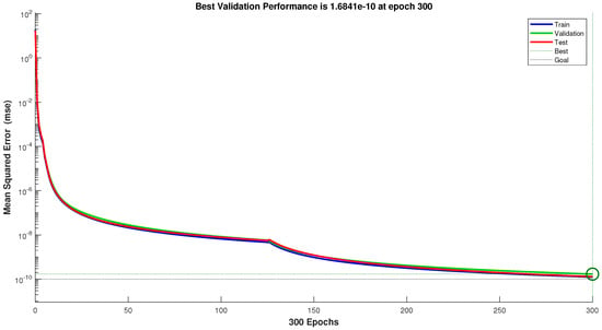
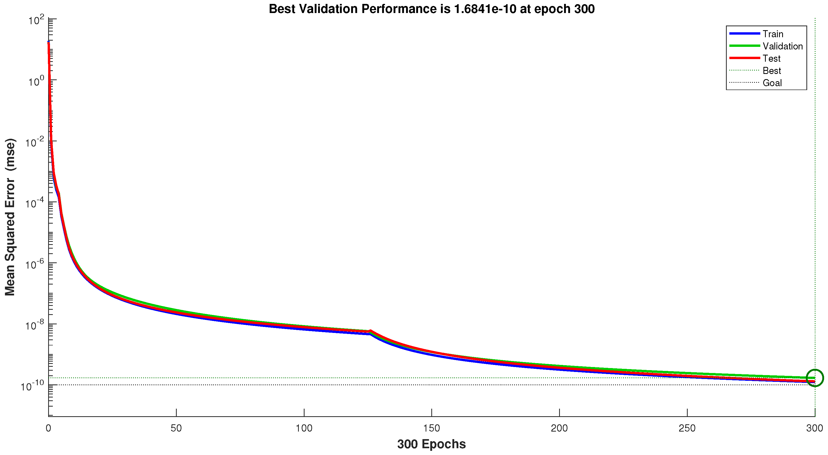
Figure 1 showcases that the learning rate of the proposed ANN model is stable and achieves the optimal value of mean square error 1.6841 at 300 epochs using all under-consideration functions. All the curves representing training, testing and validations demonstrate the same behavior during learning process.
Figure 1.
Performance of ANN structure based on mean square error.
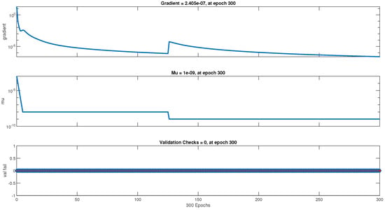
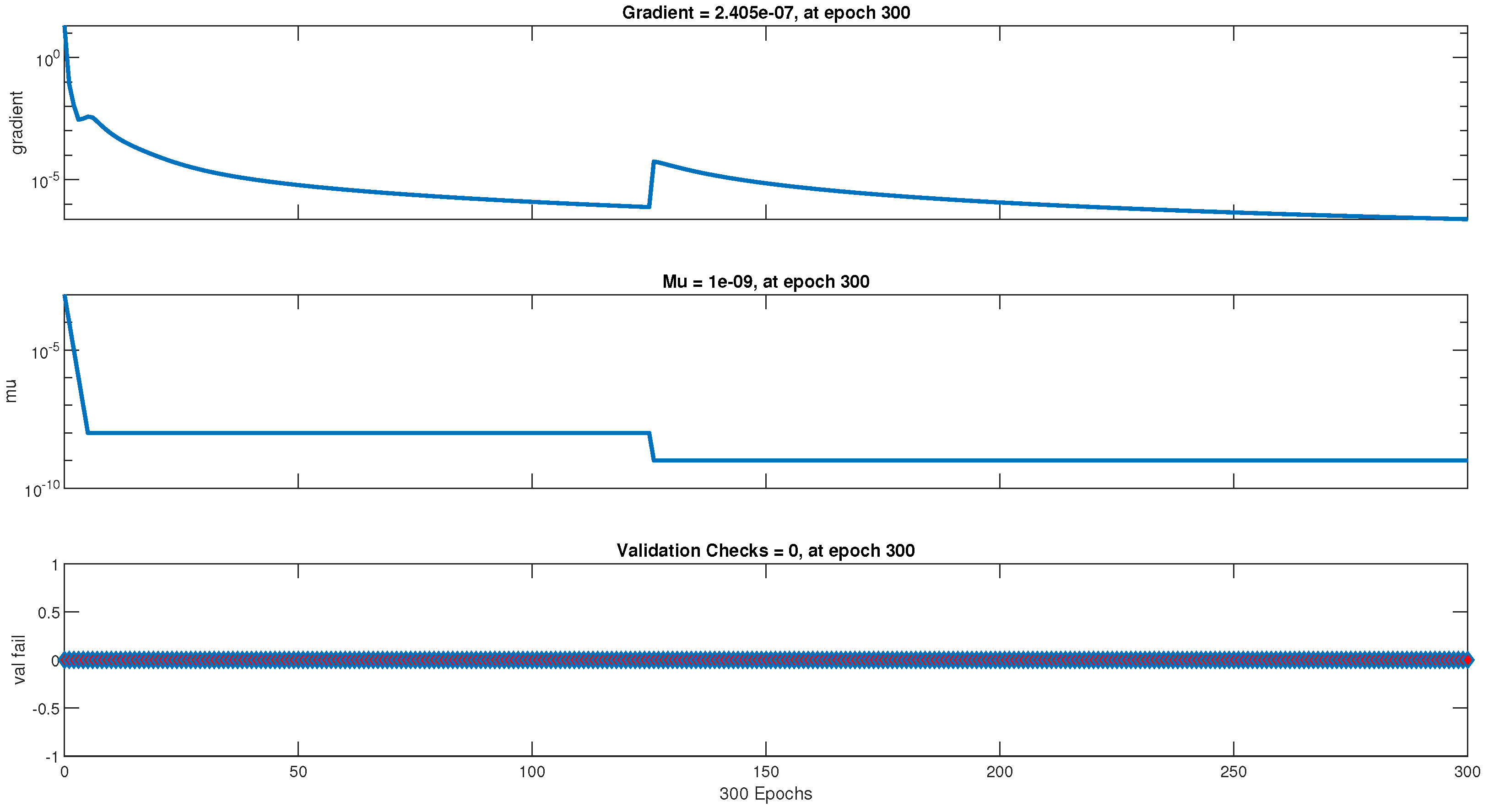
The training stages with respect to gradient values and damping value mu is discussed in Figure 2. It is a common fact that low gradient values indicate the highly stable and convergence of the ANN architecture. That is why the continuous decrement in gradient values and mu in Figure 2 confirms the stability and convergence.
Figure 2.
Training of ANN model across the values of gradient and mu and valid checks.
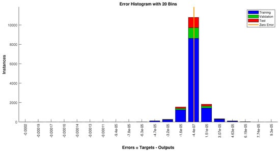
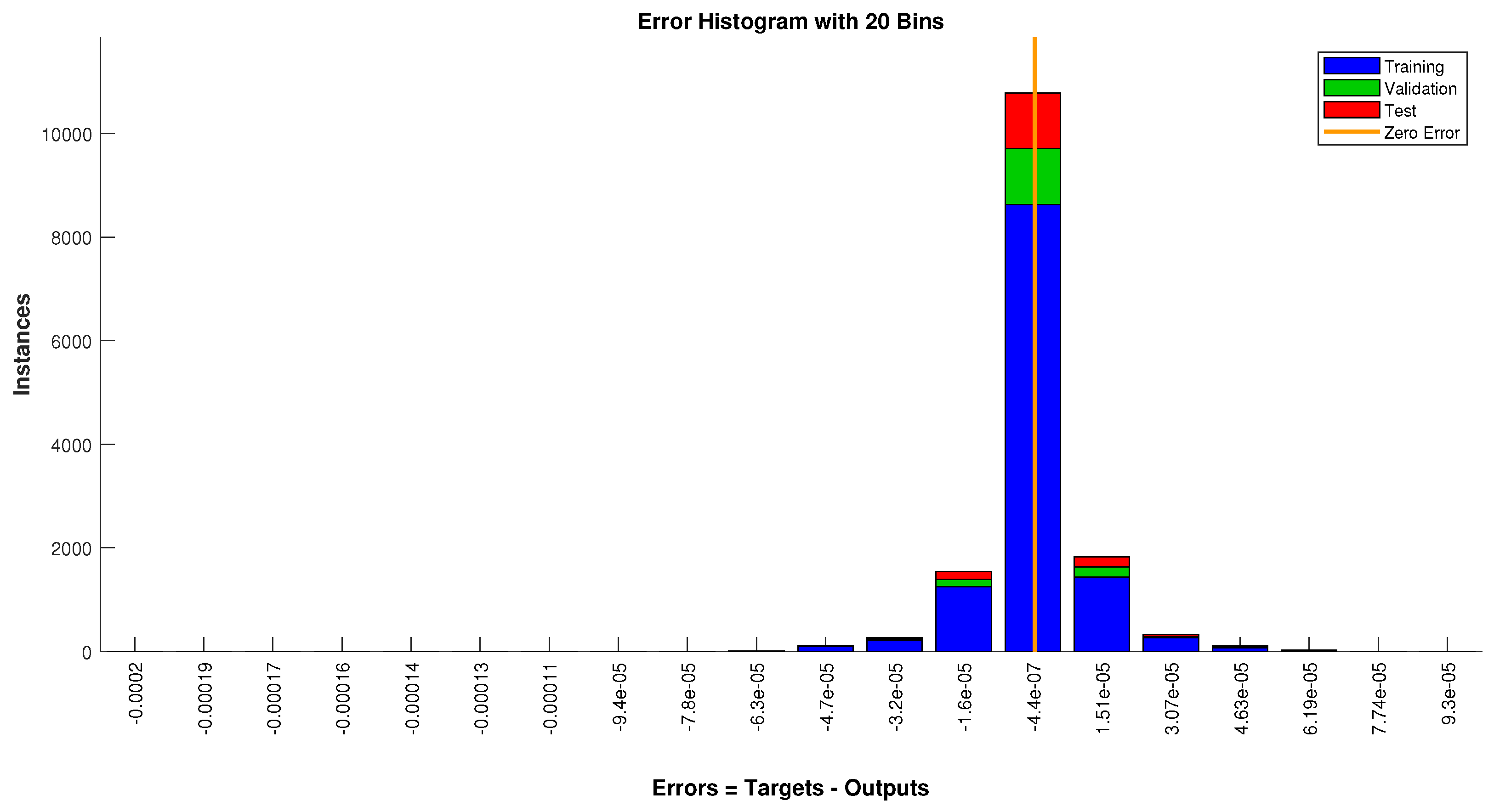
The distribution of error across 20 bins is another ANN profile, and its accuracy is provided in Figure 3. The zero-error line is centered about a very small error , which suggests that the approximations are unbiased and consistent with exact values.
Figure 3.
Frequency distribution of error.
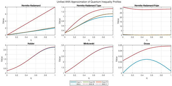
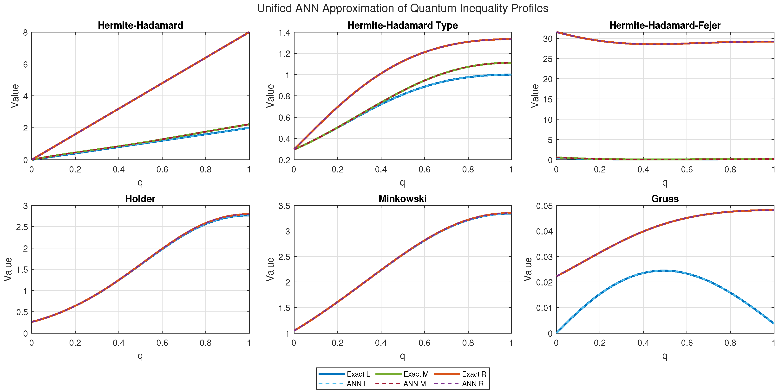
Figure 4 explicit provides the comparative analysis of each inequality between exact and ANN approximations. Clearly, the ANN approximations are preserving the inequalities. We have noticed that there is no violation and error is very low due to the use of smooth functions for data generation.
Figure 4.
Comparative analysis of all inequalities using exact approximations.
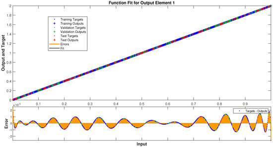
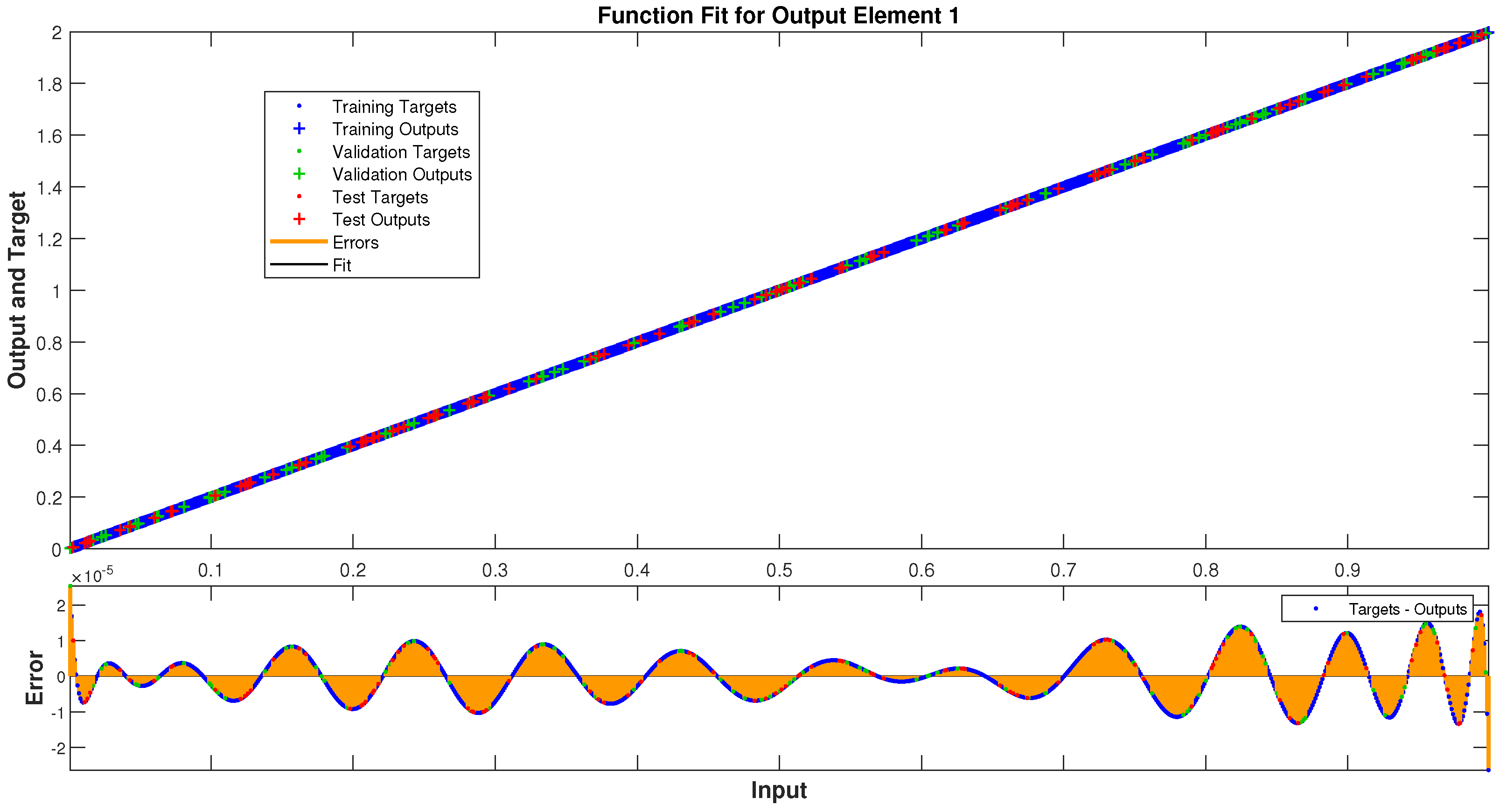
Figure 5 consists of two subplots; the first graph highlights the perfect alignment between ANN target values and simulation values. They have a linear relationship, which shows that ANN approximations are significantly accurate and the second figure focuses on the uniform oscillation of error between very small intervals. Both figures justify the robustness of the ANN model.
Figure 5.
Fitting of all target, training and validation values accurately throughout the domain of .
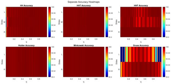
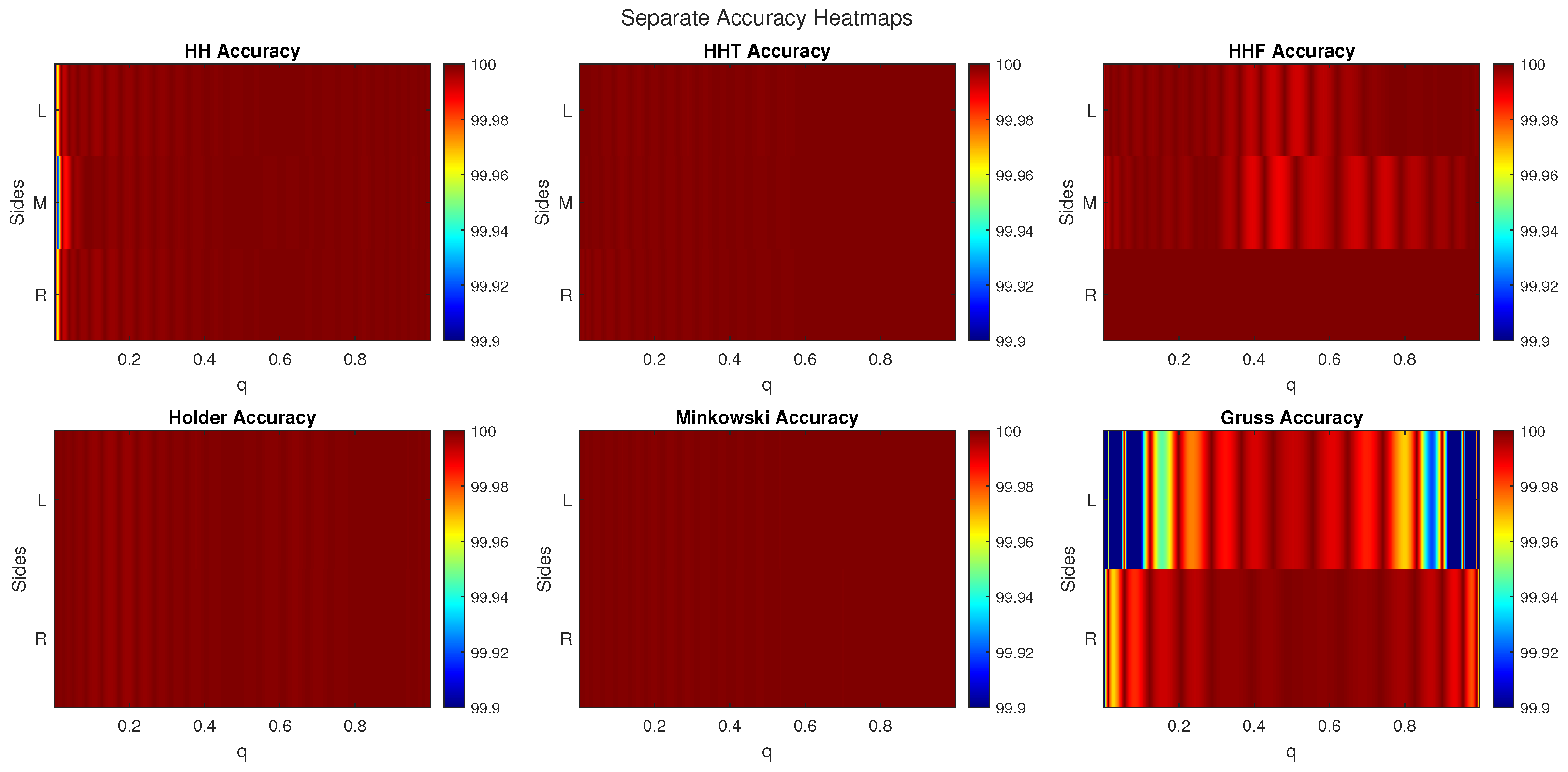
Figure 6 contains six heat maps, and each subplot is dark red, which shows that the ANN achieves an almost 100 percent accuracy level. One can also observe the accuracy of each side of inequality with the following order: left, middle and right sides.
Figure 6.
Accuracy of model against each inequality via heat maps.
The summary of ANN performance profiles are given in Table 2.
Table 2.
Comprehensive network performance summary.
4. Applications
In this section, we give some applications to means based on the Hermite–Hadamard-type inequalities. Now, we recall the special means for non-negative real numbers.
- 1.
- The arithmetic mean:
- 2.
- The generalized log-mean:
The following result establishes the bounds of the generalized log-mean.
Proposition 1.
Assume that all the assumption of Theorem 7 have the following inequality:
Proof.
Applying , to Theorem 7 and taking , then we get the required result. □
Proposition 2.
Assume that all the assumptions of Theorem 8 have the following inequality:
Proof.
Applying , to Theorem 8 and taking , then we get the required result. □
5. Concluding Remarks and Future Insights
Over the years, researchers have introduced the quantum operators and their related results in special functions and inequalities. The Jackson operators are known as classical operators. Due to their limitations in impulsive difference equations and inequalities over finite intervals, the quantum operators using the endpoints have been investigated. In this paper, we developed the symmetric quantum derivative and definite integral operators using the arbitrary point of a closed interval . They generalize the existing symmetric operators by using appropriate values of . Furthermore, we discussed the various structural properties of both operators. From an application perspective, we have proved various foundational inequalities under convexity assumptions and newly developed calculus. Additionally, we bridged symmetric quantum analytical inequalities and artificial neural networks for computational analysis. For this purpose, we established a unified feed-forward Levenberg–Marquardt ANN model using specific functions to generate the dataset. Furthermore, the detailed dynamical analysis of the ANN structure has been examined, including learning processes based on different parameters, error analysis via heat maps, and comparative analysis of ANN approximations and exact values. In the future, a wide range of inequalities and optimization problems can be investigated under the proposed framework. One can discuss the coordinated versions of the under-consideration operators and inequalities. The post-quantum, -quantum, and several other operators can be investigated following the similar technique. Furthermore, future studies should explore the directional and set-valued derivative and integral operators using an arbitrary point of a closed interval. The proposed calculus can be extended to symmetric quantum fractional derivative and integral operators. For more details, see [24]. We hope that this study will generate new insights in mathematical analysis.
Author Contributions
Conceptualization, M.Z.J., N.N. and M.U.A.; methodology, M.Z.J., L.J., M.A.; software, N.N., M.U.A. and L.J.; validation, M.Z.J., N.N., M.U.A. and M.A.; formal analysis, N.N., M.U.A., L.J. and M.A.; investigation, M.Z.J., M.U.A. and L.J.; writing—original draft preparation, M.Z.J., N.N., L.J. and M.A.; writing—review and editing, M.Z.J., N.N. and M.A.; visualization, N.N., M.U.A. and L.J.; supervision, M.U.A. All authors have read and agreed to the published version of the manuscript.
Funding
This research received no external funding.
Data Availability Statement
The original contributions presented in this study are included in the article. Further inquiries should be directed to the corresponding author.
Acknowledgments
The authors would like to acknowledge the Deanship of Graduate Studies and Scientific Research, Taif University for funding this work. The authors are thankful to the editor and the anonymous reviewers for their valuable comments and suggestions.
Conflicts of Interest
The authors declare no conflicts of interest.
References
- Jackson, F.H. On q-functions and a Certain Difference Operator. Trans. R. Soc. Edinb. 1909, 46, 253–281. [Google Scholar] [CrossRef] [Scilit]
- Jackson, F.H. On q-Definite Integrals. Q. J. Pure Appl. Math. 1910, 41, 193–203. [Google Scholar]
- Kac, V.G.; Cheung, P. Quantum Calculus; Springer: New York, NY, USA, 2002; Volume 113. [Google Scholar]
- Tariboon, J.; Ntouyas, S.K. Quantum calculus on finite intervals and applications to impulsive difference equations. Adv. Differ. Equ. 2013, 2013, 282. [Google Scholar] [CrossRef] [Scilit]
- Kunt, M.; Baidar, A.; Sanli, Z. Some quantum integral inequalities based on left-right quantum integrals. Turk. J. Sci. Technol. 2022, 17, 343–356. [Google Scholar] [CrossRef] [Scilit]
- Bilal, M.; Iqbal, A.; Rastogi, S. Quantum symmetric analogues of various integral inequalities over finite intervals. J. Math. Inequal. 2023, 17, 615–627. [Google Scholar] [CrossRef] [Scilit]
- Vivas-Cortez, M.; Javed, M.Z.; Awan, M.U.; Dragomir, S.S.; Zidan, A.M. Properties and applications of symmetric quantum calculus. Fractal Fract. 2024, 8, 107. [Google Scholar] [CrossRef] [Scilit]
- Tariboon, J.; Ntouyas, S.K. Quantum integral inequalities on finite intervals. J. Inequal. Appl. 2014, 2014, 121. [Google Scholar] [CrossRef] [Scilit]
- Xu, P.; Ihsan Butt, S.; Ain, Q.U.; Budak, H. New Estimates for Hermite-Hadamard inequality in Quantum Calculus via (α,m) convexity. Symmetry 2022, 14, 1394. [Google Scholar] [CrossRef] [Scilit]
- Kantalo, J.; Wannalookkhee, F.; Nonlaopon, K.; Budak, H. Some quantum integral inequalities for (p,h)-convex functions. Mathematics 2023, 11, 1072. [Google Scholar] [CrossRef] [Scilit]
- Adil Khan, M.; Mohammad, N.; Nwaeze, E.R.; Chu, Y.M. Quantum Hermite-Hadamard inequality by means of a Green function. Adv. Differ. Equ. 2020, 2020, 99. [Google Scholar] [CrossRef] [Scilit]
- Noor, M.A.; Awan, M.U.; Noor, K.I. Quantum Ostrowski inequalities for q-differentiable convex functions. J. Math. Inequal. 2016, 10, 1013–1018. [Google Scholar] [CrossRef] [Scilit]
- Ali, M.A.; Fečkan, M.; Mateen, A. Study of Quantum Ostrowski-Type Inequalities for Differentiable Convex Functions. Ukr. Math. J. 2023, 75, 5–28. [Google Scholar] [CrossRef] [Scilit]
- Almutairi, O.B. Quantum estimates for different type intequalities through generalized convexity. Entropy 2022, 24, 728. [Google Scholar] [CrossRef] [Scilit] [PubMed]
- Du, T.S.; Luo, C.Y.; Yu, B. Certain quantum estimates on the parameterized integral inequalities and their applications. J. Math. Inequal. 2021, 15, 201–228. [Google Scholar] [CrossRef] [Scilit]
- Nosheen, A.; Ijaz, S.; Khan, K.A.; Awan, K.M.; Albahar, M.A.; Thanoon, M. Some q-symmetric integral inequalities involving s-convex functions. Symmetry 2023, 15, 1169. [Google Scholar] [CrossRef] [Scilit]
- Liu, Q.; Javed, M.Z.; Awan, M.U.; Ciurdariu, L.; Alkahtani, B.S. Hermite-Hadamard’s like inequalities via symmetric quantum calculus. Ain Shams Eng. J. 2025, 16, 103372. [Google Scholar] [CrossRef] [Scilit]
- Butt, S.I.; Aftab, M.N.; Nabwey, H.A.; Etemad, S. Some Hermite-Hadamard and midpoint type inequalities in symmetric quantum calculus. AIMS Math. 2024, 9, 5523–5549. [Google Scholar] [CrossRef] [Scilit]
- Javed, M.Z.; Naeem, N.; Awan, M.U.; Wang, Y.; Alsalami, O.M. A Symmetric Quantum Perspective of Analytical Inequalities and Their Applications. Mathematics 2025, 13, 2910. [Google Scholar] [CrossRef] [Scilit]
- An, Y.; Ali, M.A.; Murtaza, G.; Budak, H.; Zhao, D. Some new quantum derivatives and integrals with their applications in integral error bounds. Demonstr. Math. 2025, 58, 20250161. [Google Scholar] [CrossRef] [Scilit]
- Hyder, A.A.; Budak, H.; Aly, A.M.; Abdelsalam, S.I. Exploring fractional Bullen-type inequalities via second-derivative bounds and artificial neural networks. Eng. Appl. Artif. Intell. 2025, 162, 112619. [Google Scholar] [CrossRef] [Scilit]
- Alanzi, A.R.A.; Al-Hazmy, M.; Fakhfakh, R.; Saleh, W.; Ben Makhlouf, A.; Lakhdari, A. A comprehensive analysis of proportional Caputo-hybrid fractional inequalities and numerical verification via artificial neural networks. Fractal Fract. 2026, 10, 247. [Google Scholar] [CrossRef] [Scilit]
- Javed, M.Z.; Awan, M.U.; Ciurdariu, L.; Grecu, E.; Mostafa, H. ANN-assisted sharp bounds for higher-order Euler–Maclaurin inequalities. Axioms 2026, 15, 358. [Google Scholar] [CrossRef] [Scilit]
- Wongsantisuk, P.; Ntouyas, S.K.; Passary, D.; Tariboon, J. Hilfer Fractional Quantum Derivative and Boundary Value Problems. Mathematics 2022, 10, 878. [Google Scholar] [CrossRef] [Scilit]

Disclaimer/Publisher’s Note: The statements, opinions and data contained in all publications are solely those of the individual author(s) and contributor(s) and not of MDPI and/or the editor(s). MDPI and/or the editor(s) disclaim responsibility for any injury to people or property resulting from any ideas, methods, instructions or products referred to in the content. |
© 2026 by the authors. Licensee MDPI, Basel, Switzerland. This article is an open access article distributed under the terms and conditions of the Creative Commons Attribution (CC BY) license.