Feedback Linearization of a Reduced Chemostat Model Under Inflow Disturbances

Abstract

This paper investigates the stabilization of a chemostat system with biomass settling dynamics using feedback linearization and model reduction techniques. The original three-dimensional system, composed of substrate, free biomass, and settled biomass compartments, is reduced to a two-dimensional system by assuming quasi-steady-state for the settled biomass population. A nonlinear feedback control law for the dilution rate is then designed using feedback linearization, aiming to regulate the free biomass concentration around a desired set point. The proposed control strategy compensates for nonlinearities introduced by Monod-type microbial growth and biomass settling effects. To evaluate robustness, time-varying disturbances are introduced into the inflow substrate concentration. Numerical simulations in MATLAB confirm that the closed-loop system maintains stability and tracks the biomass target despite sustained inflow fluctuations. The results demonstrate the efficacy of the reduced-order feedback linearization approach in chemostat stabilization and its potential for bioreactor control under uncertain environmental conditions.

1. Introduction

Chemostats serve as vital models in systems biology and biotechnology for studying microbial growth under nutrient-limited, continuous-flow conditions. They have been used extensively to investigate ecological competition, population stability, and the effects of environmental perturbations. However, many microbial systems display structural complexity due to spatial heterogeneity or the coexistence of multiple phenotypes, such as free-floating and surface-attached (settled) biomass. Modeling such dynamics often leads to nonlinear and high-dimensional systems that pose challenges for both analysis and control.

From a control perspective, nonlinearities in microbial growth—particularly Monod-type kinetics—require advanced methods beyond traditional linear controllers. A notable approach is to apply the mathematical methods of differential geometric nonlinear control theory, especially techniques referred to as feedback linearization [1,2,3], which transforms a nonlinear system into an equivalent linear form via nonlinear state feedback and coordinate transformation. Ballyk and Barany [4] applied this technique to chemostats, showing how feedback linearization combined with model reduction could stabilize microbial populations effectively.

The goal for using control techniques to stabilize systems is to stabilize them to a state where both species coexist at equilibrium, which can be interpreted in light of the competitive exclusion principle which states that at most one species can win the competition for resources. This makes the chemostat a very interesting system on which to apply geometric control techniques. See for example [5,6,7], for other related works investigating the use of control theory techniques to achieve the coexistence state in chemostat.

In practical settings, chemostats are often subject to environmental variability, including fluctuations in nutrient inflow concentrations. Robust control under such disturbances remains a key concern. Robustification strategies have been proposed by Nowzari and Cortés [8] for ecological systems and by Kazantzis and Kravaris [9] for general nonlinear processes, offering complementary perspectives.

Recent studies have extended feedback linearization to actuator fault-tolerant control and systems with time delays. For example, Phan et al. [3] developed a fault-tolerant controller for electro-hydraulic actuators using time delay estimation and feedback linearization, demonstrating robust tracking and fault compensation. Other works have explored feedback linearization of multi-input nonlinear systems via time scaling and prolongation, further broadening its applicability in complex control scenarios.

Recent ecological models, such as the work of Cai and Geritz [10], apply adaptive dynamics to describe microbial settlement strategies in structured chemostats, highlighting the role of site choice and competition in evolutionary outcomes. These models point to the importance of considering biomass attachment and detachment in both ecological theory and reactor design. We apply the feedback linearization method to their model to stabilize it.

In this paper, we apply the mathematical methods of differential geometry known as feedback linearization [2,4,6,7,11,12,13] and focus on a reduced-order chemostat model with biomass settling, derived under the assumption of fast attachment–detachment dynamics. The resulting two-dimensional system captures the core dynamics of substrate and free biomass concentrations, while implicitly accounting for settled biomass effects. We design a feedback-linearizing control law for the dilution rate that regulates the free biomass around a desired setpoint. Additionally, we introduce time-dependent disturbances to the inflow substrate concentration and investigate the system’s robustness via MATLAB R2023b simulations.

Our goal is to regulate the floating biomass concentration $F\left(t\right)$ in the chemostat to a desired setpoint $F^{*}$ by adjusting the dilution rate $D\left(t\right)$ while ensuring system stability, avoiding washout, and respecting operational constraints. This objective guides the design and analysis of our feedback-linearization controller and provides a basis for assessing robustness under various disturbances.

Our results demonstrate that the reduced-order feedback linearization approach provides an effective and computationally efficient means of stabilizing complex microbial systems in the presence of environmental fluctuations. This work contributes to the broader effort to develop biologically informed and theoretically grounded control strategies for nonlinear bioreactors. It is worth mentioning that systems that are feedback linearizable with known parameters and complete state observations are exactly, not approximately, analytically equivalent to linear systems when suitable nonlinear controllers are applied. This equivalence is exact, not an approximation, enabling the use of linear control design techniques to achieve a broad range of control objectives. In this work, we reduce the model dimension, apply feedback linearization, and characterize the singular region analytically and numerically.

The remainder of this paper is structured as follows. Section 2 provides preliminaries and a mathematical background on feedback linearization, the nonlinear control method employed in this study. Section 3 introduces the chemostat model with one resource and two microbial species, together with the notation used throughout. In Section 4, we discuss dimensional reduction of the model and establish conditions under which feedback linearization can be applied to the reduced system. Section 5 develops the feedback linearization control design for the reduced dynamics, while Section 6 restricts the analysis to the unconditional Bourgeois (uB) settling strategy. Finally, Section 7 concludes the paper by summarizing the main contributions of this work.

2. Preliminaries

Based on the well-written review of literature provided in the appendix for [7], we discuss some preliminary mathematical knowledge about the feedback linearization method used in this work. A control system is a dynamical system in which certain parameters can be manipulated in time to achieve specified goals, such as stabilization. Control systems may evolve in discrete or continuous time; in this work, we focus on continuous-time systems described by ordinary differential equations. Let $x\left(t\right)\in {\mathbb{R}}^n$ denote the state vector and $u\left(t\right)\in {\mathbb{R}}^p$ the control input vector. A general nonlinear control system can be written as

$$\dot{x}=f(x,u).$$

(1)

A common and useful case is the control-affine form:

$$\dot{x}=f\left(x\right)+\sum _{k=1}^p{g}_k\left(x\right)u_k,$$

(2)

where f is the drift vector field and $g_k$ are the control vector fields associated with inputs $u_k$. Non-affine systems can often be transformed into affine form through appropriate redefinition of the controls.

In feedback control, the control inputs $u\left(t\right)$ are determined in real time from measurements of the current state. Feedback is particularly effective for stabilization tasks. For example, in the second-order linear system

$$\ddot{x}+x=u,$$

(3)

stabilization to a desired state $x_0$ can be achieved using the proportional–derivative (PD) control law

$$u=x-\alpha (x-x_0)-\beta \dot{x},$$

(4)

where $\alpha ,\beta >0$ are gains. The first term cancels the natural dynamics, while the proportional and derivative terms introduce restoring and damping effects, respectively.

When dealing with nonlinear systems, linearization around an equilibrium using a Taylor expansion is effective only locally. Feedback linearization, by contrast, can achieve an exact transformation of a nonlinear system into an equivalent linear one (in new coordinates) via a state-dependent coordinate change and an appropriate feedback law. This method can, in some cases, provide stabilization over much larger regions of the state space.

The applicability of feedback linearization depends on the relative degree vector $(r_1,r_2,\dots ,r_p)$, which must satisfy the following:

• ${\sum }_{j=1}^p{r}_j=n$,
• There exist p independent output functions $h_j$, such that

  $$L_{g_j}{L}_f^l{h}_k=0,0\le l<r_k-1,$$
• The decoupling matrix

  $$A_{jk}=L_{g_j}{L}_f^{r_k-1}{h}_k$$

  has full rank.

Here, $L_{f}h$ denotes the Lie derivative of h along f:

$$L_f^{0}h=h,L_f^{l+1}h=\nabla \left(L_f^{l}h\right)·f.$$

When these conditions hold, the system can be transformed into Brunovský normal form, in which each output is governed by an independent chain of integrators:

$${\dot{z}}_{j,1}=z_{j,2},\dots ,{\dot{z}}_{j,r_j-1}=z_{j,r_j},$$

(5)

$${\dot{z}}_{j,r_j}=v_j,j=1,\dots ,p,$$

(6)

where $v_j$ are new linear control inputs. This form allows the direct application of linear control techniques such as PD or pole placement to the transformed system.

3. Model Description

We consider a structured chemostat environment hosting a polymorphic microbial population, where each species is characterized by a distinct settling rate $x_i$. Microbial individuals may exist either as floaters F, suspended in the fluid, or as settlers S, attached to the chemostat wall. Both subpopulations consume a common limiting nutrient R, which supports microbial growth.

The growth of floaters and settlers is modeled by the functions $f_F\left(R\right)$ and $f_S\left(R\right)$, respectively, which are assumed to be continuous and increasing with $f_F\left(0\right)=f_S\left(0\right)=0$. A typical choice is the Monod form:

$$f_F\left(R\right)={\displaystyle \frac{{\mu }_{F}R}{{\nu }_F+R}},f_S\left(R\right)={\displaystyle \frac{{\mu }_{S}R}{{\nu }_S+R}},$$

where ${\mu }_F,{\mu }_S$ are maximal growth rates, and ${\nu }_F,{\nu }_S$ are half-saturation constants for floaters and settlers, respectively (see Table 1).

Table 1. Definitions of state variables and model parameters.

Symbol	Description	Unit
$R\left(t\right)$	concentration of nutrients at time t	g × cm−3
$F\left(t\right)$	biomass concentration of floaters	g × cm−3
$S\left(t\right)$	areal biomass density of settlers	g × cm−2
Y	yield constant	-
${\mu }_F,{\mu }_S$	maximal growth rates	t−1
${\nu }_F,{\nu }_S$	half-saturation constants	g × cm−3 or cm−2
${\delta }_F,{\delta }_S$	death rates of floaters and settlers	t−1
$x_i$	settling rate of species i	t−1
K	maximum settler biomass density	g × cm−2
a	habitable surface area	cm2
D	dilution rate	t−1
$R_{\mathrm{in}}$	input nutrient concentration	g × cm−3
$R_{\mathrm{in}}^0$	average input nutrient concentration (periodic case)	g × cm−3

Spatial limitations impose an upper bound K on settler biomass. The transition from floaters to settlers is governed by the settling functions $g(x,S)$ and $h(x,S)$, where g describes the landing attempt rate and h denotes the successful settlement rate. The following ODE system models the chemostat dynamics:

$$\begin{array}{c}\dot{R}=-{\displaystyle \frac{1}{Y}}\left(f_F\left(R\right)F+f_S\left(R\right)S\right)+D\left(R_{\mathrm{in}}-R\right),\hfill \\ \dot{F}=f_F\left(R\right)F+f_S\left(R\right)S-{\delta }_{F}F-g(x,S)F-DF,\hfill \\ \dot{S}=h(x,S)F-{\delta }_{S}S-DS,\hfill \end{array}$$

(7)

with $R_{\mathrm{in}}$ constant and $D\left(t\right)$ the possibly time-varying dilution rate. Here, R, F, and S denote nutrient, floater biomass, and settler biomass concentrations, respectively. Since the organism is the same in the model, one anticipates that the yield constants are equal whether the microbe is in its floating state or its settled state [10,14]. Here, we write the substrate–biomass model in a mass-balanced form (we keep the common yield $Y>0$, which may be removed by scaling; below we keep Y explicit). The term $-DS$ in this model accounts for the removal of surface-attached microbes due to medium flow or washout. It ensures that the dynamics of attached biomass reflect both mortality and dilution, allowing the model to capture realistic total biomass and resource balance under continuous flow.

The yield Y can be eliminated from the substrate equation by rescaling the biomass variables. Define

$$\tilde{F}:={\displaystyle \frac{F}{Y}},\tilde{S}:={\displaystyle \frac{S}{Y}}.$$

If the original model is written with reciprocal yields in the substrate equation,

$$\dot{R}=-{\displaystyle \frac{1}{Y}}\left(f_F\left(R\right)F+f_S\left(R\right)S\right)+D(R_{\mathrm{in}}-R),$$

then, after substituting $F=Y\tilde{F}$, $S=Y\tilde{S}$, the substrate equation becomes

$$\dot{R}=-f_F\left(R\right)\tilde{F}-f_S\left(R\right)\tilde{S}+D(R_{\mathrm{in}}-R),$$

and the biomass equations retain their form but with any occurrence of S replaced by $Y\tilde{S}$. In particular, for settling functions of the form $g(x,S)=x(1-S/K)$ and $h(x,S)=x(1-S/K)$, one may equivalently set $\tilde{K}:=K/Y$ and obtain the same functional dependence in $(\tilde{F},\tilde{S})$. Thus, without loss of generality we set $Y=1$ and work with the scaled biomass variables (denoted $F,S$ again), noting that dimensional biomass values are recovered by multiplying by Y.

Mainly, there are three ecological settlement strategies of ecological interest, each corresponding to distinct biological assumptions [10]:

• The unconditional Bourgeois (uB) settling

  $$g(x,S)=x,h(x,S)=x\left(1-{\displaystyle \frac{S}{K}}\right)$$

  and floaters land indiscriminately. If the site is occupied, the resident repels the intruder.
• The unconditional anti-Bourgeois (uaB) settling

  $$g(x,S)=x,h(x,S)=x\left(1-{\displaystyle \frac{S}{K}}\right)$$
  Floaters land freely and displace any existing settlers. The intruder always wins.
• The Biological (b-) settling

  $$g(x,S)=x\left(1-{\displaystyle \frac{S}{K}}\right),h(x,S)=x\left(1-{\displaystyle \frac{S}{K}}\right)$$
  Floaters only target vacant sites, leading to declining settlement rates as space becomes scarce.

System (7) assumes that both floating and settled microbes consume the common substrate R, but with different uptake functions $f_F\left(R\right)$ and $f_F\left(R\right)$ reflecting their physiological states and spatial limitations. Floating cells experience full mixing, while settled cells are diffusion-limited on the wall surface. This split uptake structure is standard in chemostat models with wall attachment (see for example [14,15,16]). In our formulation, settled biomass serves as a refuge and does not produce new floaters, so its growth term is absent from the floating biomass equation.

In the monomorphic case (single species), $g(x,S)$ and $h(x,S)$ are independent of F. The uB and uaB strategies yield identical dynamics since they produce the same functional forms in this setting. In contrast, the b-settling mechanism produces distinct behavior because both landing and success rates depend explicitly on wall saturation $S/K$. This leads to nonlinear feedback effects that shape population dynamics and settlement stability [10].

In the case of a single limiting resource and two competing microbial species, these strategy-dependent dynamics provide the foundation for the feedback control and stabilization analysis. For clarity of exposition, we focus on the unconditional Bourgeois (uB) settling strategy, as the primary objective is to illustrate the methodology of feedback linearization rather than to investigate the ecological consequences of alternative settling strategies.

• Equilibrium and Basic Reproduction Number:

The equilibrium points are as follows: The washout equilibrium $E_0=(R_{in},0,0)$ and the positive equilibrium $E_{*}=(R_{*},F_{*},S_{*})$. The basic reproductive number ${\mathcal{R}}_0$ is defined as the expected number of successful offspring (i.e., new settlers or floaters that remain in the system) produced by a single microorganism introduced into an otherwise uncolonized or uninfected chemostat. Applying the Next Generation Method [14]. Let $\mathcal{P}=(R,F,S)$, then model (7) can be rewritten as ${\mathcal{P}}^{\prime }=\tilde{F}\left(\mathcal{P}\right)-\tilde{V}\left(\mathcal{P}\right)$, where the matrices $\tilde{F}$ and $\tilde{V}$ represent respective new infection and transition, and they are given by the population dynamics of x in the virgin environment (i.e., at the washout equilibrium $E_0$) as

$$\left(\begin{array}{c}\dot{F}\\ \dot{S}\end{array}\right)=\left(\begin{array}{cc}{f}_F\left(R_{\mathrm{in}}\right)-D-{\delta }_F-x& f_S\left(R_{\mathrm{in}}\right)\\ x& -({\delta }_S+D)\end{array}\right)\left(\begin{array}{c}F\\ S\end{array}\right),$$

which is the same for all other settling mechanisms.

The partial derivatives of f with respect to $(F,S)$, evaluated at the washout equilibrium $E_0$, are denoted as $F_0$ and $V_0$, respectively:

$${\mathcal{F}}_0=\left(\begin{array}{cc}{f}_F\left(R_{\mathrm{in}}\right)& f_S\left(R_{\mathrm{in}}\right)\\ 0& 0\end{array}\right),{\mathcal{V}}_0=\left(\begin{array}{cc}D+{\delta }_F+x& 0\\ -x& {\delta }_S+D\end{array}\right).$$

Hence,

$$F_0{V}_0^{-1}=\left(\begin{array}{cc}{\displaystyle \frac{({\delta }_S+D)f_F\left(R_{\mathrm{in}}\right)+x{f}_S\left(R_{in}\right)}{({\delta }_S+D)(D+{\delta }_F+x)}}& {\displaystyle \frac{f_S\left(R_{in}\right)}{{\delta }_S}}\\ 0& 0\end{array}\right)$$

Therefore, the basic reproduction number is ${\mathcal{R}}_0={\displaystyle \frac{({\delta }_S+D)f_F\left(R_{\mathrm{in}}\right)+x{f}_S\left(R_{in}\right)}{({\delta }_S+D)(D+{\delta }_F+x)}}.$ For a detailed stability analysis of system (7), we direct the reader to the appendix of [10].

4. Feedback Linearization of the Reduced System

The full chemostat model, including nutrient and population dynamics, often leads to a high-dimensional nonlinear system that may not satisfy the accessibility conditions required for global feedback linearization. This issue has been thoroughly analyzed in [4], where the authors demonstrate that for two competing microbial species and two essential resources, the four-dimensional system fails to satisfy the necessary accessibility conditions asymptotically.

To overcome a similar challenge in our model, we follow their methodology and reduce the system dimension by exploiting an invariant manifold resulting from the system’s asymptotic behaviour. Specifically, from the mass balance dynamics, the following constraint holds asymptotically:

$$R\left(t\right)=R_{\mathrm{in}}-{\displaystyle \frac{F\left(t\right)}{Y}}-{\displaystyle \frac{S\left(t\right)}{Y}},$$

(8)

where Y is the growth yield common constant for the floating and settled populations. Using this relationship, we eliminate the nutrient concentration $R\left(t\right)$ from the model, leading to a reduced three-dimensional system in terms of $(F,S)$. This simplification facilitates the application of feedback linearization to design a stabilizing controller for the reduced system.

To stabilize the reduced chemostat system, we apply differential geometric control theory via feedback linearization. The goal is to transform the nonlinear dynamics into a linear controllable system using an appropriate change of coordinates and feedback law.

Following the standard procedure, we write the reduced system as an affine control system:

$$\dot{x}=f\left(x\right)+ug\left(x\right),$$

(9)

where x is the state vector, u is the control input (e.g., dilution rate D), and f, g are smooth vector fields. We seek an output function $\varphi \left(x\right)$ such that the system has a well-defined relative degree and satisfies the feedback linearization conditions (see for example [17]).

The relative degree is determined by iteratively differentiating $\varphi \left(x\right)$ along the vector fields until the control u appears explicitly. The transformed system can then be written in Brunovsky normal form, and standard linear control techniques (e.g., PD control) can be applied to achieve stabilization.

The specific linearizing coordinates and feedback law depend on the choice of output function, which we construct based on biologically meaningful quantities such as species ratios or total biomass.

System (7) can be written as an affine control system:

$$\dot{\mathbf{x}}=\mathbf{f}\left(\mathbf{x}\right)+\sum _{i=1}^2{u}_i{\mathbf{g}}_i\left(\mathbf{x}\right)$$

(10)

where $\mathbf{x}={(R,F,S)}^{\top }$, the control vector fields are

$${\mathbf{g}}_1\left(\mathbf{x}\right)=\left(\begin{array}{c}1\\ 0\\ 0\end{array}\right),{\mathbf{g}}_2\left(\mathbf{x}\right)=\left(\begin{array}{c}-R\\ -F\\ 0\end{array}\right).$$

The drift vector field is given by the following:

$$\mathbf{f}\left(\mathbf{x}\right)=\left(\begin{array}{c}-f_F\left(R\right)F-f_S\left(R\right)S\\ f_F\left(R\right)F+f_S\left(R\right)S-{\delta }_{F}F-g(x,S)F\\ h(x,S)F-{\delta }_{S}S\end{array}\right).$$

Lemma 1.

The system

$$\dot{\mathbf{x}}=\mathbf{f}\left(\mathbf{x}\right)+u_1{\mathbf{g}}_1\left(\mathbf{x}\right)+u_2{\mathbf{g}}_2\left(\mathbf{x}\right)$$

is feedback linearizable if

$$\begin{array}{cc}\hfill \det ({\mathbf{g}}_1,{\mathbf{g}}_2,{\mathrm{ad}}_{\mathbf{f}}{\mathbf{g}}_1,{\mathrm{ad}}_{\mathbf{f}}{\mathbf{g}}_2)& ={(R_{\mathrm{in}}-R)}^{2}FS\left({\displaystyle \frac{\partial f_F}{\partial R}}{\displaystyle \frac{\partial h}{\partial S}}-{\displaystyle \frac{\partial f_F}{\partial S}}{\displaystyle \frac{\partial h}{\partial R}}\right)\hfill \\ \hfill & +(R_{\mathrm{in}}-R)FS\left[\left({\displaystyle \frac{\partial f_F}{\partial S}}+{\displaystyle \frac{\partial f_S}{\partial S}}\right)\left({\displaystyle \frac{\partial h}{\partial R}}-{\displaystyle \frac{\partial f_F}{\partial R}}\right)\right.\hfill \\ \hfill & +\left.\left({\displaystyle \frac{\partial f_F}{\partial R}}+{\displaystyle \frac{\partial f_S}{\partial R}}\right)\left({\displaystyle \frac{\partial f_F}{\partial S}}-{\displaystyle \frac{\partial h}{\partial S}}\right)\right]\ne 0.\hfill \end{array}$$

(11)

The functions $f_F\left(R\right)$, $f_S\left(R\right)$, $g(x,S)$, and $h(x,S)$ are assumed to be smooth, and the partial derivatives are taken with respect to the indicated variables. The involved condition ensures that the vector fields and their Lie brackets span the required space to allow for feedback linearization. The determinant being nonzero implies that the system has full relative degree and is locally diffeomorphic to a controllable linear system.

Figure 1 illustrates the critical behavior of the system with respect to the resource concentration R, specifically focusing on the condition under which feedback linearization may fail. The plotted curve represents the difference between the derivatives of the uptake functions for the floating and wall-settled microbial populations, given by ${\displaystyle \frac{d{f}_F}{dR}}-{\displaystyle \frac{d{f}_S}{dR}}$. These functions characterize the rate at which each population consumes the single limiting nutrient R, and their derivatives play a central role in the accessibility and linearizability of the system.

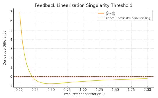
Figure 1. Difference between the derivatives of the uptake functions for floaters and settlers, ${\displaystyle \frac{d{f}_F}{dR}}-{\displaystyle \frac{d{f}_S}{dR}}$, plotted against the resource concentration R. The red dashed line marks the zero crossing, which corresponds to the singular value $\hat{R}$ where the accessibility matrix becomes degenerate and feedback linearization fails. This critical threshold delineates regions in the state space where linearizing control laws are valid from regions where they break down.

The red dashed line indicates the zero-crossing of this difference, marking a singular threshold where the determinant of the accessibility matrix becomes zero. At this point, the coordinate transformation and control law used in feedback linearization break down, as the system loses full relative degree and the required Lie bracket structure degenerates. This singularity has a direct consequence: it divides the state space into regions where feedback linearization is well-posed and regions where it fails. Therefore, any controller designed using feedback linearization must either ensure that system trajectories avoid this singular point or incorporate a switching or hybrid strategy to transition across it safely. This highlights the importance of identifying and characterizing singular values of the resource variable in single-resource chemostat models.

This following lemma ensures that the total resource and microbial biomass converge to a predictable mass balance. It highlights that, under continuous dilution, the system reaches a steady state in which the combined amount of remaining resource and microbial biomass is determined by the inflow concentration, providing a foundation for analyzing microbial persistence and population dynamics.

Lemma 2.

For any solution $\left(R\right(t),F(t),S(t\left)\right)$ of the system (7), we have

$$\underset{t\to \infty }{\lim }\left(R\left(t\right)-R_{\mathrm{in}}+{\displaystyle \frac{F\left(t\right)}{Y}}+{\displaystyle \frac{S\left(t\right)}{Y}}\right)=0.$$

(12)

Proof. 

Define the quantity

$$\theta \left(t\right)=R\left(t\right)-R_{\mathrm{in}}+{\displaystyle \frac{F\left(t\right)}{Y}}+{\displaystyle \frac{S\left(t\right)}{Y}}.$$

(13)

Differentiating $\theta$ along the trajectories of the system and substituting the equations of motion yields

$${\displaystyle \frac{d\theta }{dt}}=-D\left(t\right)\theta \left(t\right)-{\displaystyle \frac{1}{Y}}[({\delta }_F+g(x,S)-h(x,S))F+{\delta }_{S}S]$$

(14)

where $D\left(t\right)$ is the dilution rate, assumed to be a control input. Since the second term on the right-hand side of (14) is always non-positive, we have

$${\displaystyle \frac{d\theta }{dt}}\le -D\left(t\right)\theta \left(t\right).$$

(15)

Suppose that $D\left(t\right)\ge ϵ>0$ for all t. Then, by Grönwall’s inequality,

$$\theta \left(t\right)\le \theta \left(0\right)·\exp \left(-{\int }_0^{t}D\left(s\right)ds\right)\le \theta \left(0\right)e^{-ϵt}.$$

(16)

Hence,

$$\underset{t\to \infty }{\lim }\theta \left(t\right)=0,$$

which implies that

$$\underset{t\to \infty }{\lim }\left(R\left(t\right)-R_{\mathrm{in}}+{\displaystyle \frac{F\left(t\right)}{Y}}+{\displaystyle \frac{S\left(t\right)}{Y}}\right)=0.$$

□

In nonlinear control theory, feedback linearization relies on the assumption that the vector fields associated with the system’s inputs and their Lie brackets with the drift field span the full state space. A necessary condition for this transformation to be well-defined is that the determinant of the so-called accessibility matrix is non-zero. Violation of this condition results in a loss of relative degree and renders the system non-feedback-linearizable in that region.

For the chemostat model under consideration, with a single resource R, floaters F, and settlers S, feedback linearizability depends critically on the structure of the uptake function $f_F(R,S)$ and the settlement function $h(x,S)$. Specifically, the system fails to be feedback linearizable when the following expression vanishes:

$$\Delta (R,S)={\displaystyle \frac{\partial f_F}{\partial R}}·{\displaystyle \frac{\partial h}{\partial S}}-{\displaystyle \frac{\partial f_F}{\partial S}}·{\displaystyle \frac{\partial h}{\partial R}}=0.$$

(17)

This defines a curve or surface in the $(R,S)$ state space that separates feedback linearizable regions from non-linearizable ones. Inside the linearizable region (i.e., where $\Delta (R,S)\ne 0$), a nonlinear feedback transformation can render the system fully linear. Outside of this region, such a transformation becomes singular or undefined, and alternate control strategies are required.

Figure 2 illustrates the feedback linearizable region (shaded green), and the singular boundary where $\Delta (R,S)=0$ (red curve). The functions used here for illustration are Monod-type uptake and saturation functions:

$$f_F\left(R\right)={\displaystyle \frac{2R}{1+R}}+0.1S,h(x,S)={\displaystyle \frac{1.5S}{1+S}}.$$

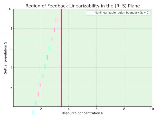
Figure 2. Region of feedback linearizability in the $(R,S)$ state space. Green area: states where the system can be feedback-linearized. Red curve ($\Delta (R,S)=0$): boundary where linearizability is lost.

The region to the left of the red curve is non-linearizable due to the singularity in the feedback transformation. This highlights the importance of understanding the geometry of the state space when designing controllers, as trajectories that evolve toward this singular set may lead to failure or instability in the control response.

5. Feedback Linearization Control Design

To stabilize the reduced chemostat dynamics, we apply feedback linearization to the two-dimensional system derived earlier. Let $F\left(t\right)$ and $S\left(t\right)$ denote the concentrations of floaters and settlers, respectively. Using the asymptotic mass balance condition, the effective nutrient concentration is given by

$$R\left(t\right)=R_{\mathrm{in}}-{\displaystyle \frac{F\left(t\right)}{Y}}-{\displaystyle \frac{S\left(t\right)}{Y}}.$$

(18)

Substituting this into the model leads to the reduced two-dimensional system:

$$\begin{array}{c}\dot{F}=f_F\left(R_{\mathrm{eff}}\right)F+f_S\left(R_{\mathrm{eff}}\right)S-({\delta }_F+D+g(x,S))F,\hfill \\ \dot{S}=h(x,S)F-({\delta }_S+D)S,\hfill \end{array}$$

(19)

where $f_F$ and $f_S$ are nutrient uptake functions, g and h are settling terms, and D is the dilution rate serving as the control input.

To regulate the system, we aim to stabilize the floater population $F\left(t\right)$ at a desired reference value $F^{*}$ by manipulating the dilution rate $D\left(t\right)$, while ensuring stability, avoiding washout, and respecting operational constants. We define a virtual control v using a proportional-derivative (PD) structure:

$$v=-k_1(F-F^{*})-k_2\dot{F},$$

(20)

where $k_1,k_2>0$ are controller gains.

Rewriting Equation (19) to solve for the dilution rate D, and substituting $\dot{F}=v$, yields the feedback linearizing control law:

$$D={\displaystyle \frac{1}{F}}\left[f_F\left(R_{\mathrm{eff}}\right)F+f_S\left(R_{\mathrm{eff}}\right)S-{\delta }_{F}F-g(x,S)F-v\right].$$

(21)

This expression defines the required dilution rate D that renders the nonlinear system linear in the new coordinates and drives the floater population to the desired level $F^{*}$.

Lemma 3.

The reduced chemostat system is feedback linearizable in regions of the $(F,S)$-plane, where

$${\displaystyle \frac{\partial f_F\left(R\right)}{\partial R}}\ne {\displaystyle \frac{\partial f_S\left(R\right)}{\partial R}},$$

evaluated at $R=R_{\mathrm{in}}-{\displaystyle \frac{F}{Y}}-{\displaystyle \frac{S}{Y}}$.

Proof. 

Consider the reduced system:

$$\begin{array}{c}\dot{F}=f_F\left(R(F,S)\right)F+f_S\left(R(F,S)\right)S-({\delta }_F+D+g(x,S))F,\hfill \\ \dot{S}=h(x,S)F-({\delta }_S+D)S.\hfill \end{array}$$

(22)

Define the output function $\varphi \left(F\right)=\ln \left(F\right)$. Then,

$$\dot{\varphi }={\displaystyle \frac{1}{F}}\dot{F}=f_F\left(R\right)+{\displaystyle \frac{S}{F}}{f}_S\left(R\right)-({\delta }_F+D+g(x,S)).$$

(23)

For feedback linearization to be valid, the second derivative of $\varphi$ must depend explicitly on D, and the decoupling matrix must be nonsingular. The condition $\partial f_F/\partial R\ne \partial f_S/\partial R$ ensures sufficient sensitivity of the system to D, guaranteeing invertibility of the transformation. □

Remark 1.

The curve defined by $f_F\left(R\right)=f_S\left(R\right)$ partitions the $(F,S)$-plane into three regions: $f_F\left(R\right)>f_S\left(R\right)$, Region II: $f_F\left(R\right)<f_S\left(R\right)$, and Region III: $f_F\left(R\right)=f_S\left(R\right)$.

In Regions I and II, the inequality $\partial f_F/\partial R\ne \partial f_S/\partial R$ holds, allowing feedback linearization. However, along the boundary in Region III, this condition fails, and the feedback transformation becomes singular. Biologically, this corresponds to the scenario where floaters and settlers respond identically to nutrient availability, rendering control via D ineffective. Hence, feedback linearization is only applicable locally in regions satisfying the sensitivity condition.

Figure 3 verifies Lemma 1 numerically. The singular locus (black contour) represents points in the $(F,S)$-plane where $\Delta \left(R\right)=0$, and the system loses feedback linearizability due to identical nutrient sensitivity between floaters and settlers. The colored background indicates the sign and magnitude of $\Delta \left(R\right)$, highlighting regions of feasible control.

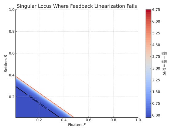
Figure 3. Contour plot of $\Delta \left(R\right)={\displaystyle \frac{\partial f_F}{\partial R}}-{\displaystyle \frac{\partial f_S}{\partial R}}$ over the $(F,S)$-state space. The black contour labeled “Singular Locus” shows where feedback linearization fails. The system is only locally linearizable in regions where $\Delta \left(R\right)\ne 0$.

The second singularity condition involves a critical value $\hat{R}$, defined by

$$\Delta (R,S)={\displaystyle \frac{\partial f_F}{\partial R}}·{\displaystyle \frac{\partial h}{\partial S}}-{\displaystyle \frac{\partial f_F}{\partial S}}·{\displaystyle \frac{\partial h}{\partial R}}=0.$$

(24)

This defines a singular surface in the $(R,S)$-space. The point $\hat{R}$ lies on this surface and marks the loss of feedback (Figure 4).

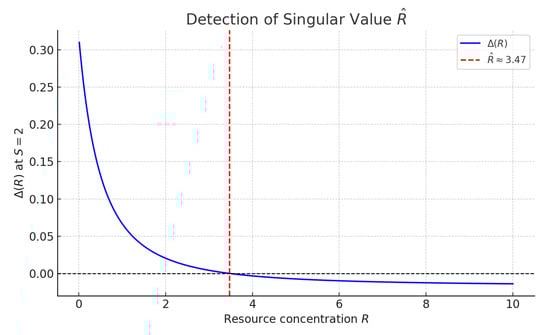
Figure 4. Detection of the critical settler population $\hat{S}$ where $\Delta \left(S\right)=0$, evaluated at fixed $R=3.0$. The red dashed line marks the threshold between linearizable and non-linearizable regimes.

The singular locus $\Delta (R,S)=0$ acts as an approximate boundary between physical equilibria (feasible population levels) and unphysical ones (e.g., negative biomass). It is not merely a mathematical artifact—it provides geometric insight into the system’s basin of attraction. Control strategies based on feedback linearization must therefore be confined to regions away from this boundary to ensure stability and biological relevance [18].

6. Feedback Linearization for Unconditional Bourgeois (uB) Settling

We now consider the reduced chemostat model with Unconditional Bourgeois (uB) settling, where

$$g(x,S)=x,h(x,S)=x\left(1-{\displaystyle \frac{S}{K}}\right),$$

(25)

and the dilution rate $u:=D$ is the control input. After substituting the asymptotic mass-balance relation

$$R_{\mathrm{eff}}=R_{\mathrm{in}}-{\displaystyle \frac{F}{Y}}-{\displaystyle \frac{S}{Y}},$$

(26)

the two-dimensional reduced system becomes

$$\begin{array}{c}\dot{F}=f_F\left(R_{\mathrm{eff}}\right)F+f_S\left(R_{\mathrm{eff}}\right)S-({\delta }_F+D+x)F,\hfill \\ \dot{S}=x\left(1-{\displaystyle \frac{S}{K}}\right)F-({\delta }_S+D)S.\hfill \end{array}$$

(27)

This can be written in affine control form $\dot{z}=f\left(z\right)+g\left(z\right)u$ with $z={(F,S)}^{\top }$, where

$$f\left(z\right)=\left(\begin{array}{c}{f}_F\left(R_{\mathrm{eff}}\right)F+f_S\left(R_{\mathrm{eff}}\right)S-({\delta }_F+x)F\\ x\left(1-{\displaystyle \frac{S}{K}}\right)F-({\delta }_S+D)S\end{array}\right),g\left(z\right)=\left(\begin{array}{c}-F\\ 0\end{array}\right).$$

Lemma 4.

For the reduced chemostat model (19) with uB settling, the output

$$y=\ln F$$

has relative degree $r=1$ for all $F>0$. The input–output linearizing control law

$$D=f_F\left(R_{\mathrm{eff}}\right)+{\displaystyle \frac{S}{F}}{f}_S\left(R_{\mathrm{eff}}\right)-({\delta }_F+x)-v$$

(28)

yields the linear input–output relation $\dot{y}=v$.

Proof. 

The gradient of y is $\nabla y=(1/F,0)$, so

$$L_{g}y=\nabla y·g={\displaystyle \frac{1}{F}}(-F)=-1\ne 0,$$

(29)

showing that the relative degree is $r=1$ and that the control appears in the first derivative of y. The Lie derivative along f is

$$L_{f}y=f_F\left(R_{\mathrm{eff}}\right)+{\displaystyle \frac{S}{F}}{f}_S\left(R_{\mathrm{eff}}\right)-({\delta }_F+x),$$

(30)

hence

$$\dot{y}=L_{f}y+u{L}_{g}y=f_F\left(R_{\mathrm{eff}}\right)+{\displaystyle \frac{S}{F}}{f}_S\left(R_{\mathrm{eff}}\right)-({\delta }_F+x)-D.$$

(31)

Choosing D according to (28) enforces $\dot{y}=v$.   □

To regulate F to a desired setpoint $F^{*}$, we choose

$$v=-k\left(\ln F-\ln F^{*}\right),k>0,$$

(32)

which yields $\dot{y}=-k(y-y^{*})$ and ensures exponential convergence $F\left(t\right)\to F^{*}$.

When $F\left(t\right)\equiv F^{*}$, the S-dynamics reduce to

$$\dot{S}=-\left({\delta }_S+D+{\displaystyle \frac{x{F}^{*}}{K}}\right)S+x{F}^{*},$$

(33)

a linear, globally asymptotically stable ordinary differential equation with equilibrium

$$S^{*}={\displaystyle \frac{x{F}^{*}}{{\delta }_S+D+\frac{x{F}^{*}}{K}}}.$$

(34)

Thus, the internal dynamics are stable for all biologically feasible parameters (Figure 5).

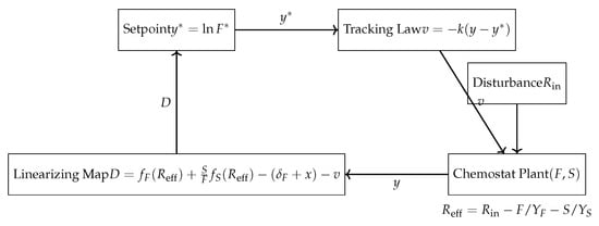
Figure 5. Block diagram of the feedback-linearizing control system for the chemostat. The input is the dilution rate D, the output is floater biomass F (or $y=\ln F$), and the disturbance is inflow substrate concentration $R_{\mathrm{in}}$.

Note that the relative degree $r=1$ means the method achieves input–output linearization, not full-state feedback linearization. This is sufficient for the regulation of F. In addition, the zero dynamics are globally stable, ensuring the full state $(F,S)$ converges to $(F^{*},S^{*})$ provided $D\left(t\right)\ge 0$ and $F\left(t\right)>0$. Also, the practical implementation requires enforcing $D\ge 0$ (e.g., by saturation) and avoiding F near zero to preserve the logarithmic output definition.

7. Conclusions

This study introduces a nonlinear control framework to stabilize reduced chemostat dynamics via feedback linearization, accounting for environmental disturbances such as inflow fluctuations. Starting from a biologically grounded chemostat model incorporating Monod-type kinetics and species-specific wall-settling behavior, we derived a reduced-order system by leveraging a quasi-steady-state approximation of the nutrient concentration.

We applied differential geometric control theory to this reduced two-dimensional system, constructing a state feedback control law using feedback linearization. A proportional-derivative (PD) controller was implemented in the transformed coordinates to regulate the floater population around a prescribed setpoint. The analysis identified critical conditions under which the system is locally feedback linearizable—namely, when the nutrient sensitivities of floaters and settlers are distinct. These conditions were further explored through the concept of a singular locus, which delineates regions in state space where linearizing control is valid versus regions where it fails. A comprehensive, experimentally validated study of environmental variability—such as temperature, pH, and dissolved oxygen effects—represents an important direction for future research.

Numerical simulations demonstrated the effectiveness of the control strategy, showing robust tracking performance under time-varying perturbations in nutrient inflow. The proposed approach provides a biologically interpretable and mathematically rigorous tool for controlling microbial ecosystems with limited sensing or actuation.

The feedback linearization strategy developed in this work is particularly relevant for real-world bioreactor systems where maintaining stable microbial populations is essential under fluctuating environmental conditions. For example, in industrial fermentation and wastewater treatment processes, the ability to regulate biomass concentrations in response to disturbances such as variable nutrient inflow or environmental shocks can significantly improve process efficiency and reliability. Our control law can be implemented using standard sensors to monitor substrate and biomass levels, and actuators to adjust the dilution rate in real time. This approach provides robustness against environmental fluctuations and model uncertainties, making it suitable for practical deployment in automated bioreactor control systems. By enabling precise regulation of microbial populations, the proposed method supports enhanced productivity, resilience, and adaptability in diverse microbial ecosystems.

Although feedback linearization provides exact input–output linearization under ideal conditions, it fails near singularities where the determinant of the accessibility (decoupling) matrix approaches zero. To address this limitation in practical applications, singularity-aware supervisory schemes can be integrated into the control framework. For example, the controller can monitor the determinant and, when it falls below a predefined threshold, switch to a reference governor that slows setpoint changes or transitions to a robust or adaptive control law. Additionally, techniques such as dynamic extension (adding an integrator to the input) or redefining the regulated output can enlarge the linearizable domain and help avoid instability near singularities. These hybrid strategies preserve stability and constraint feasibility while maintaining the benefits of feedback linearization in the nominal region. In response to the reviewer’s suggestion, we have expanded the discussion to include these practical approaches, referencing foundational works such as [17,19].

This work highlights the promise of geometric nonlinear control methods in managing complex bio-processes. Future extensions could explore multi-species systems, incorporate state estimation under output constraints, or integrate adaptive mechanisms to cope with parametric uncertainties and unmodeled dynamics.

References

- De Leenheer, P.; Smith, H. Feedback control for chemostat models. J. Math. Biol. 2003, 46, 48–70. [Google Scholar] [CrossRef] [PubMed]
- Henson, M.A.; Seborg, D.E. Nonlinear control strategies for continuous fermenters. Chem. Eng. Sci. 1992, 47, 821–835. [Google Scholar] [CrossRef]
- Pilyugin, S.S.; Waltman, P. The simple chemostat with wall growth. Siam J. Appl. Math. 1999, 59, 1552–1572. [Google Scholar] [CrossRef]
- Ballyk, M.; Barany, E. Stabilization of chemostats using feedback linearization and reduction of dimension. In Proceedings of the 2009 American Control Conference, St. Louis, MO, USA, 10–12 June 2009; pp. 2313–2318. [Google Scholar]
- Mazenc, F.; Malisoff, M.; Harmand, J. Further Results on Stabilization of Periodic Trajectories for a Chemostat with Two Species. IEEE Trans. Autom. Control 2008, 53, 66–74. [Google Scholar] [CrossRef]
- Ballyk, M.; Barany, E. The role of resource types in the control of chemostats using feedback linearization. Ecol. Model. 2008, 211, 25–35. [Google Scholar] [CrossRef]
- Phan, V.; Vo, C.; Dao, H.; Ahn, K. Actuator Fault-Tolerant Control for an Electro-Hydraulic Actuator Using Time Delay Estimation and Feedback Linearization. IEEE Access 2021, 9, 106830–106845. [Google Scholar] [CrossRef]
- Nowzari, C.; Cortés, J. Team-triggered coordination for real-time control of networked cyber-physical systems. Automatica 2016, 68, 237–247. [Google Scholar] [CrossRef]
- Kazantzis, N.; Kravaris, C. Nonlinear observer design using Lyapunov’s auxiliary theorem. Syst. Control Lett. 1998, 34, 241–247. [Google Scholar] [CrossRef]
- Cai, Y.; Geritz, S. Understanding site choice and competition through the adaptive dynamics of settling rate evolution in a chemostat. bioRxiv 2020. [Google Scholar] [CrossRef]
- Nijmeijer, H.; van der Schaft, A.J. Nonlinear Dynamical Control Systems; Springer: New York, NY, USA, 1990. [Google Scholar]
- Vidyasagar, M. Nonlinear Systems Analysis; SIAM: Philadelpia, PA, USA, 2002. [Google Scholar]
- Kravaris, K.; Kantor, J.C. Geometric methods for nonlinear process control. Backgr. Ind. Eng. Chem. Res. 1990, 29, 2295–2310. [Google Scholar] [CrossRef]
- Martcheva, M. An Introduction to Mathematical Epidemiology; Springer: New York, NY, USA, 2015. [Google Scholar]
- Stemmons, E.; Smith, H.L. Competition in a chemostat with wall attach-ment. Siam J. Appl. Math. 2000, 61, 567–595. [Google Scholar] [CrossRef]
- Ballyk, M.; Jones, D.; Smith, H.L. The biofilm model of Freter: A review. In Structured Population Models in Biology and Epidemiology; Springer: Berlin/Heidelberg, Germany, 2008; pp. 265–302. [Google Scholar]
- Isidori, A. Nonlinear Control Systems, 3rd ed.; Springer: London, UK, 1996. [Google Scholar]
- Qi, X.; Henson, M.A. Nonlinear model predictive control of a continuous fermentation process. J. Process Control 1998, 8, 217–227. [Google Scholar]
- Kravaris, C.; Wright, R.A.; McIntosh, S.C. Nonlinear state feedback control of chemical pro-cesses: A tutorial review. Processes 2013, 1, 30–54. [Google Scholar]
Disclaimer/Publisher’s Note: The statements, opinions and data contained in all publications are solely those of the individual author(s) and contributor(s) and not of MDPI and/or the editor(s). MDPI and/or the editor(s) disclaim responsibility for any injury to people or property resulting from any ideas, methods, instructions or products referred to in the content. |
© 2025 by the authors. Licensee MDPI, Basel, Switzerland. This article is an open access article distributed under the terms and conditions of the Creative Commons Attribution (CC BY) license (https://creativecommons.org/licenses/by/4.0/).