
On Robustness for Spatio-Temporal Data


Departamento de Estadística, I.O. y C.N., Universidad Nacional de Educación a Distancia (UNED), Senda del Rey 9, 28040 Madrid, Spain
Mathematics 2022, 10(10), 1785; https://doi.org/10.3390/math10101785
Submission received: 19 April 2022
/
Revised: 13 May 2022
/
Accepted: 18 May 2022
/
Published: 23 May 2022
(This article belongs to the Special Issue Probability Theory and Stochastic Modeling with Applications)
Abstract
:The spatio-temporal variogram is an important factor in spatio-temporal prediction through kriging, especially in fields such as environmental sustainability or climate change, where spatio-temporal data analysis is based on this concept. However, the traditional spatio-temporal variogram estimator, which is commonly employed for these purposes, is extremely sensitive to outliers. We approach this problem in two ways in the paper. First, new robust spatio-temporal variogram estimators are introduced, which are defined as M-estimators of an original data transformation. Second, we compare the classical estimate against a robust one, identifying spatio-temporal outliers in this way. To accomplish this, we use a multivariate scale-contaminated normal model to produce reliable approximations for the sample distribution of these new estimators. In addition, we define and study a new class of M-estimators in this paper, including real-world applications, in order to determine whether there are any significant differences in the spatio-temporal variogram between two temporal lags and, if so, whether we can reduce the number of lags considered in the spatio-temporal analysis.
Keywords:
robust statistics; spatio-temporal outliers; von Mises expansions; saddlepoint approximationsMSC:
62F35; 62H11; 62E171. Introduction
There exist several approaches for the treatment of spatio-temporal data. The most common approach is to assume that the data are a partial realization of a spatio-temporal random field , (see, e.g., [1,2]). In this superpopulation model ([3], p. 8), we also assume that D is a fixed subset of , and ; that is, we assume that a random variable Z, such as precipitation, temperature or atmospheric pollutant concentrations, is observed at some known fixed locations and different time moments t, considering a geostatistical framework where the spatial observations are expected to be correlated with a decreasing correlation as the distance between locations increases.
We can conduct exploratory data analysis with spatio-temporal data, mainly through their visualization. However, it is more interesting to model the random field, allowing for inference of the model parameters and closed-form expressions (see [4]). As it is usually assumed that the data come from a joint Gaussian (i.e., normal) distribution, we are interested in estimating the parameters; that is, summaries of the first- and second-order characteristics. To make this feasible, we suppose that is intrinsically stationary in space and time; that is, its increments in space and time have a zero mean (possibly after a temporal trend has been removed) and have a variance that depends only on displacements in space and differences in time. With these assumptions, the parameter of interest is the spatio-temporal variogram of Z, defined as
where is the variance of Z, is a spatial lag, and is a temporal lag.
We also assume that Z is spatially isotropic; that is, the variogram depends on the spatial lag h only through the Euclidean norm .
Furthermore, one of the most important problems in geostatistics is kriging prediction at new locations, for which the spatio-temporal variogram is required. Hence, the spatio-temporal variogram is the crucial parameter in geostatistics. However, the traditional spatio-temporal variogram estimator, which is commonly employed for these purposes, is extremely sensitive to outliers. Moreover, in a wide range of fields, such as geology, the environment, sustainability or climate change, detecting atypical observations is of special interest.
Considering these aims, we first define new robust estimators of the spatio-temporal variogram. Then, we obtain very accurate approximations for the sample distribution of these new estimators, and, with these, we finally identify spatio-temporal outliers.
The spatio-temporal variogram of Z can also be written as
where E denotes the mathematical expectation of Z.
To analyze Z, we consider observations of the random field at spatial locations and times , where is the sample size.
In this situation, the spatio-temporal variogram is estimated using the classical method-of-moments estimator, also called the empirical spatio-temporal variogram (see [3,5,6]),
where refers to the set containing all pairs of spatial locations with spatial lag , and refers to the set containing all pairs of time points with time lag . Furthermore, denotes the number of elements in the set .
If we denote, by , the sample size considered in the estimator —that is, the number of pairs with spatio-temporal lag —this estimator is a sample mean of terms and, hence, sensitive to outliers in the terms.
In [7], robust estimators of the spatial variogram and accurate approximations for their distributions were obtained. In [8], these results were extended to the multivariate case, with robust estimators for the cross-variogram. In the first part of this paper, we extend these results by introducing a temporal component into the problem. This is achieved by defining new robust M-estimators of the spatio-temporal variogram and obtaining accurate approximations for their distributions, as well as for the classical one, . In the last part of this paper, we propose a method for identifying spatio-temporal outliers, also obtaining interesting properties of a new class of M-estimators.
The remainder of this paper is organized as follows: A spatio-temporal variogram M-estimator is proposed in Section 2, and an approximation to its distribution is obtained at the end of Section 3.2. The problem of independence of the transformed observations is addressed in Section 4. These results are applied in Section 5 to the empirical spatio-temporal variogram estimator. In Section 6, we introduce Huber’s spatio-temporal variogram estimator and obtain an approximation to its distribution. An example is developed in Section 7. The question of whether some temporal lags can be dropped in the analysis is considered in Section 8. The problem of identifying spatio-temporal outliers is addressed in Section 9, where a new class of M-estimators is defined. The conclusions of the paper are presented in Section 10.
2. M-Estimators of the Spatio-Temporal Variogram
2.1. Underlying Model for Z
The common model assumption for spatio-temporal data Z is a normal distribution. Nevertheless, this is a very strong assumption as, although most of the data will come from this model, it is very likely that some will not. For this reason, it is more realistic to assume a scale-contaminated normal distribution for the model (see, e.g., [9], p. 2):
where and , with representing the proportion of outliers in the sample and g denoting the quantity that contaminates them. For or , this model is the normal distribution and, if and , it is the in the central part but with heavier tails. In this way, we consider that the model for Z is inside the class of scale contamination neighborhoods of the normal distribution, , one of the usual model classes considered in robustness studies ([9] p. 12, [10,11] or [12] p. 870).
Although the main role in the question of the underlying model is played by the marginal distributions of Z, in order to complete the mathematical framework, we shall assume that these marginal distributions are obtained from the multivariate scale-contaminated normal distribution (see, e.g., [13], pp. 2, 220).
2.2. M-Estimators of the Spatio-Temporal Variogram
Let us consider the transformation
These new variables will be shortened, in some cases, by , , considering them as a sample of a new variable defined from the lags of Z in space and time. As the parameter of interest is now , the problem of estimating the spatio-temporal variogram described in the previous section can be considered as the problem of estimating the expectation of the random variable X, obtained from the original Z through this transformation.
This framework is especially suitable and useful in situations related to spatial or temporal data, where the initially dependent observations are separated by a spatial and/or temporal lag and where direct robust estimators, if they exist, are difficult to apply. Considering this mean (the spatio-temporal variogram) as a functional T of the underlying distribution F,
where F is the cumulative distribution function of X, and its classical method-of-moments estimator is the sample mean
of the transformed variables , where is the empirical cumulative distribution function. This approach—that is, expressing estimators as functionals of the empirical distribution function—is common and useful in robustness studies ([9,14]).
An important question here is how to choose the transformation (1) such that the new variables are independent in the new sample mean. We shall deal with this problem later. If we achieve this independence, obtaining robust estimators for the parameter is an easy task with M-estimators and -trimmed means of the transformed variables . With respect to the former, we can define a spatio-temporal M-estimator ([11]) for the parameter (the spatio-temporal variogram) based on the transformed observations as a solution to the equation
assuming that is monotonic decreasing in for all x. In fact, as is an estimator for a location problem, is of the form , with monotonically increasing in v. Now, we should control the local robustness of these M-estimators, through choosing different bounded score functions (see, e.g., refs. [9,15] for a background on robust methods and standard M-estimators.)
Hence, the idea that we propose in the paper is that, instead of considering a weird estimator for a strange parameter of the initial Z distribution, we transform the original (and usually dependent) observations into new data (independent under some conditions), obtaining, in this way, a natural parameter of the new variable (e.g., its mean), for which a manageable estimator (the sample mean) should be feasible. Then, standard techniques of robustification can be applied. The comparison between the traditional estimator (the empirical spatio-temporal variogram) and one of these robust M-estimators here introduced, both based on the observations , is the well-known comparison between the sample mean and a robust M-estimator (see, e.g., [9,14]).
2.3. Distribution of Variables
An important problem is to determine the distribution of this new variable X, from the original normal (or contaminated normal) distribution of Z, in order to later obtain the distribution of the robust estimators based on X.
If we consider a scale-contaminated normal model for the original observations Z, as the variable follows a normal distribution with 0 mean and variance . For each , the distribution of the transformed variables
is the mixture
where and , where is a chi-square distribution with one degree of freedom, following a similar development to that followed in [7], Section 2.1.
3. Approximation to the Distribution of M-Estimators of the Spatio-Temporal Variogram
The distribution of these new robust M-estimators , defined by (2), depends on the distribution of the new variables after the transformation. We obtain an approximation to the distribution of the robust estimators in two steps: in the first step, we consider a von Mises expansion (VOM) of the tail probability functional, which depends on another functional, for which we obtain a saddlepoint approximation (SAD) in the second step. The independence of the is now required.
3.1. Von Mises Approximation
If is an estimator with associated functional T, and F is the underlying model distribution of the observations , we usually cannot express explicitly; however, we can utilize a linearization based on the von Mises expansion, [18], at G (called the pivotal distribution) as follows:
where is the Hampel Influence Function; that is, the Gteaux derivative of T at G in direction , the Dirac measure at x (see [15,19,20]).
If we consider T as the tail probability functional, , the Hampel Influence Function is now the Tail Area Influence Function TAIF ([21]), and the previous von Mises expansion is equal to
from which we define the von Mises approximation (VOM)
which will be accurate if the distributions F and G are close. In this case, we can use this approximation to compute the distribution of under the underlying model F using a model G in the class .
In particular, if F is the mixture , the von Mises approximation will be
because
3.2. Saddlepoint Approximation of the TAIF
The von Mises approximations (3) or (4) depend on the TAIF, which is the influence function of the tail probability functional. Daniels ([22], p. 94), using the Lugannani and Rice formula ([23]), gave the following saddlepoint approximation (SAD) for the tail probability of an M-estimator with score function , assuming that G is the underlying model for the ,
where and are the cumulative and density functions of the standard normal distribution, and s and r are the functionals
where
is the cumulant generating function of the distribution G; and are the second and first partial derivatives of with respect to the first argument , respectively, and is the saddlepoint; that is, the functional solution of the saddlepoint equation
If, in approximation (5), we replace the model G by the contaminated model and obtain the derivative at , in all of the functionals involved in it, we obtain a saddlepoint approximation of the , (for details, see [24] pp. 402–404, [25] p. 77 or [9] p. 314), as
Replacing the SAD approximation (6) in the VOM approximation (3), we obtain the VOM + SAD approximation for the distribution of an M-estimator with score function , at the model F, which is on the order of ,
In the particular case that the transformed observations follow a mixture model , the VOM + SAD approximation is
Remark 1.
If the sample size is large and is asymptotically normal under F, we can approximate its distribution using the Central Limit Theorem, thereby, obtaining
Remark 2.
Approximations (7) and (8) are valid for any M-estimator with score function ψ based on data, solution of (2). For spatio-temporal data, these , which are transformations of the initial observations, have different distributions than the used in [7] for the estimation of the spatial variogram and also different from those used in [8] in the estimation of the cross-variogram.
In addition to the differences in the observations are the differences in the score functions. Here, for the spatio-temporal problem, ψ will include the temporal dimension, which was not considered in the other two mentioned papers. However, the main difference is that, in [7], we obtained M-estimators for the spatial variogram, while here we obtained it for the spatio-temporal variogram. However, if the temporal dimension is removed (see Section 8), both estimators will agree. Hence, the estimators obtained here generalize those of the variogram (without temporal dimension) obtained there, as it should be.
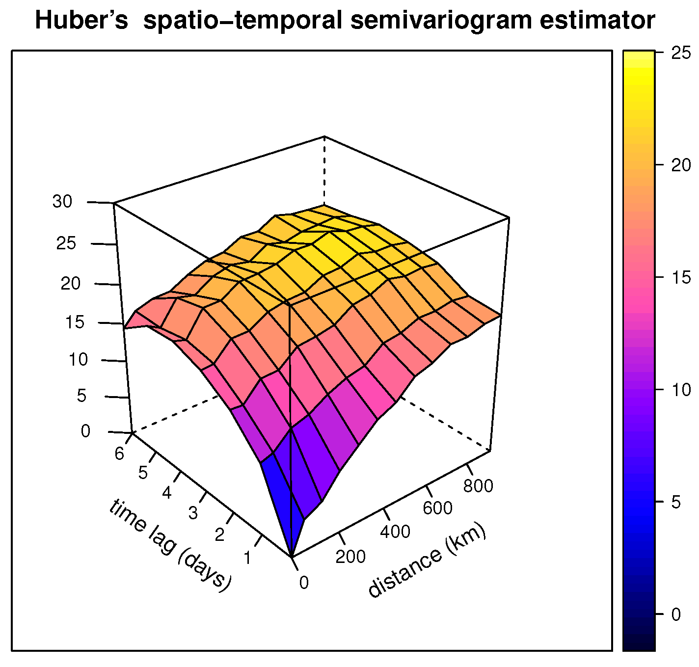
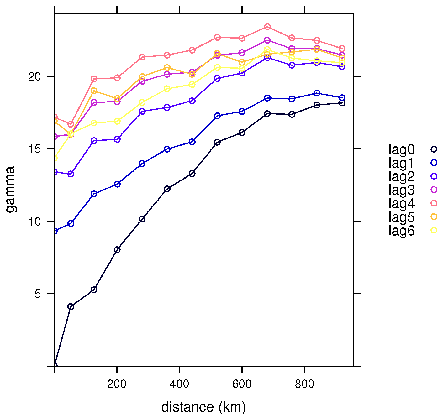
This remark can be clearly observed in the example considered in Section 7, where we obtain seven different spatial variogram estimators (see Figure 6 for the classical and Figure 7 for the robust) at the seven different temporal lags considered—all of them obtained from the only one classical (Figure 4) or robust (Figure 5) three-dimensional spatio-temporal variogram estimator.
4. Independence of the Transformed Variables
As the locations are fixed in advance, they can be considered as being equally spaced on a transect, as in [3], p. 32. Hence, we can match two contiguous (for which the dependence of the is supposed to be the strongest), such that . Under these conditions, with the same arguments as in [7], Section 2, it can be proved that, at each time and time lag , the correlation between and is 0 if a linear semivariogram model can be accepted for all the initial variables.
Moreover, following the ideas provided in [8] for the cross-variogram, if we can also accept a linear cross-variogram for each pair at any pair of time moments, assuming that all moments are equally spaced, the variables and will also be independent; then, so will all of the , , assuming that the vector of the observations is distributed as a multivariate (or contaminated) normal distribution.
Hence, to obtain the independence of the , we must check that a linear semivariogram can be accepted for the and a linear cross-variogram for each pair .
This can easily be checked in a visual way with R and formally with the global test proposed in [7], Section 10.1. Furthermore, these linearity requirements should not be a serious problem, as we can move the spatial lag and/or the time lag until linearized versions ([7], Section 9) of the variograms and cross-variograms can be accepted.
5. VOM + SAD Approximation of the Distribution of the Empirical Spatio-Temporal Estimator
As the classical method-of-moments estimator
is an M-estimator and a solution of the equation
with the score function , we can use the results of Section 3 to obtain a VOM + SAD approximation for its distribution.
In the unrealistic case of no contamination—namely, if and so, —the exact distribution of is the tail of a distribution with degrees of freedom,
Hence, using as a pivotal distribution, the von Mises approximation (8) becomes
considering a scale-contaminated normal distribution for the original observations Z, i.e., the following model for the
where and ; that is, where G is a gamma distribution with parameters , and H is a gamma distribution with parameters .
In (9), the saddlepoint is
and approximation (9) becomes
This approximation has the same accuracy as the VOM + SAD approximation obtained in [7] for Matheron’s estimator because, in fact, the classical spatio-temporal estimator is a generalization of Matheron’s estimator. For this reason, the lack of robustness of Matheron’s estimator is also inherited in the empirical spatio-temporal estimator.
Accuracy of the Approximation
Let us observe that, if or , the sum of the right-hand side of approximation (10) is zero. Moreover, we can observe the accuracy of this approximation with a simulation, as explained in the Supplementary Material.
With this simulation, we can see the quality of approximation (10) in Table 1 for several values of a, considering a sample size as small as , (i.e., contamination in scale), and . The exact values were obtained with a simulation considering samples.
This VOM + SAD approximation is shown in Figure 1, as the dotted line, where the solid line shows the exact distribution.
In Figure 2, we plot the VOM + SAD approximation with different contaminations: , , and . We can see that, as the contamination percentage (i.e., the value of ) increases, the p-values and critical values are greatly affected, graphically indicating the lack of robustness of the classical spatio-temporal estimator.
The details of this and other computations, as well as the R functions ([26]) used in the paper, are available on the website https://www2.uned.es/pea-metodos-estadisticos-aplicados/spa-temp-variogram.htm as Supplementary Material (accessed on 18 April 2022).
6. Huber’s Spatio-Temporal Variogram Estimator
We define the Huber spatio-temporal variogram estimator as the M-estimator obtained from Equation (2) using, as the score function , the Huber function , where b is the tuning constant.
This estimator is a generalization of the spatial Huber estimator for the spatial variogram defined in [7]. Here, the score function incorporates the time component, sometimes as spatial variograms at different time moments.
In the approximation proposed for the tail probability of Huber’s spatio-temporal variogram estimator, we approximate the leading term using the Lugannani and Rice formula, [23], given in (5), and the second term using the integral of the saddlepoint approximation of the TAIF obtained in Section 3.2, assuming again a scale-contaminated normal model. The VOM + SAD approximation obtained in this way is
where the saddlepoint is obtained from the saddlepoint equation
Some applications of this estimator are given in the following example.
7. Example
For this example, we obtain the Huber spatio-temporal variogram estimator for the NOAA data set. This data set was introduced in [5] and refers to the daily weather data obtained by the US National Oceanic and Atmospheric Administration (NOAA) National Climatic Data Center.
In this data set, we considered the variable Tmax—the daily maximum temperature in degrees Fahrenheit. The classical spatio-temporal semivariogram for this variable is shown in Figure 2.17 of [5], p. 39. In Figure 3, we show the Huber spatio-temporal semivariogram estimator defined in this paper, considering the tuning constant .
Three-dimensional representations of these classical and robust Huber’s spatio-temporal semivariogram estimators are shown, respectively, in Figure 4 and Figure 5.
Details of these computations are provided in the Supplementary Material.
8. Significant Time Dimension
We can see differences with respect to the selected temporal lags in Figure 6 and Figure 7 for the classical and robust semivariogram estimators, respectively, obtained from the three-dimensional spatio-temporal variogram estimators by fixing the lags. These differences became smaller as we increased the time lag. If there were no significant differences between two of these semivariograms, we could group these two lags into one, thus, reducing the number of time lags considered.
Let us denote by and the semivariograms at lags and for a fixed spatial lag , having corresponding distributions and . If we use approximation (7), considering the distributions and , the VOM + SAD approximation of the distribution of the classical spatio-temporal estimator at lag is
where is the sample size used by at spatial lag and temporal lag .
In the same way as in a general testing problem, we test the null hypothesis against the alternative using a test statistic , computing the tail probability , where is the observed value of , and if this probability is small (large), we reject (accept) the null hypothesis. Here, we can test, for a fixed spatial lag , the null hypothesis of no significant change between two temporal lags and —that is, , against —by computing the tail probability
A small value of this probability will discredit the null hypothesis and lead us to reject it, concluding that there exists a significant difference between the semivariograms at the lags and , suggesting that we must compute the (classical or robust) estimators in a separate way at these two lags. On the other hand, if we accept the null hypothesis, we shall group these two lags, thus, considering one less lag.
For instance, in the previous example, considering the spatial lag between 240 and 320, the previous probability between the starting moment and the first time lag or that between the first and second temporal lag, are both equal to 0, suggesting highly significant differences between these two pairs of lags (as can be appreciated in Figure 6 and Figure 7).
On the other hand, the probability between time lags four and five is 0.9427521 and between the last two is 0.9737844, (for the spatial lag ), leading us to accept the null hypothesis and suggesting that we can consider all of these observations in a single group for the computation of the spatio-temporal variogram estimator.
9. Identification of Spatio-Temporal Outliers
The second objective of this work is to identify spatio-temporal outliers. For this purpose, we calculated the VOM + SAD approximation of the distribution of the Difference M-estimator, an M-estimator that is essentially the difference between the classical method-of-moments estimator and the Huber estimator defined in Section 6. We chose this pair of estimators, as Huber’s estimator minimizes the maximum asymptotic variance inside the class of contamination neighborhoods of the normal distribution—the class of models considered in the paper—and the mean is an extreme particular case of it (i.e., they are nested estimators). When this difference is significant at some pair of lags, we qualify this pair of lags as spatio-temporal outliers.
This M-estimator is completely defined in (12) below; however, we can also say that the Difference M-estimator is one of the estimators inside the class defined in the next section.
9.1. Average M-Estimators
M-estimators ([11]) are likely the most widely used robust estimators. Nevertheless, they are somewhat unpleasant to handle as they are defined in an implicit way, as a solution of an equation; in particular, the spatio-temporal M-estimator is a solution of Equation (2). Next, we define a new class of M-estimators, which is considered in this paper only for the case of location estimation.
Definition 1.
If is an M-estimator with score function ψ and, thus, with M-functional defined by
the Average M-estimator associated with is defined as
with the associated functional
The Average M-estimator associated with the mean is exactly the mean and is the associated with the Huber estimator, being the Huber score function considered in Section 6.
An Average M-estimator is an M-estimator with score function because it is a solution of
that is,
or
We summarize some of the main properties of this class of M-estimators in the following proposition.
Proposition 1.
(a) The Influence Function of a linear combination of estimators is the linear combination of their Influence Functions:
If is a linear combination of q estimators with Influence Functions , the Hampel Influence Function of T is .
(b) The linear combination of Average M-estimators is an M-estimator:
If is a linear combination of q Average M-estimators with score functions , then T is an M-estimator with score function
(c) The Hampel Influence Function of an Average M-functional is
(d) The robustness properties of an Average M-estimator are the same as those of the M-estimator from which it is defined.
(e) Any Average M-functional is a linear functional and is weakly continuous on the class of probability distributions on the Borel σ-algebra if ψ is bounded.
(f) The asymptotic distribution of an Average M-estimator is normal with the mean being the associated functional and asymptotic variance
Proof.
The proof of (a) is straightforward due to the linearity properties of the limits (or derivatives) and because the Hampel Influence Function is defined as a limit.
To prove (b), we set up the equation
that is,
or
(c) The Hampel Influence Function of an Average M-functional
is obtained first by contaminating the distribution
and then obtaining the derivative at ,
(d) The infinitesimal robustness properties of an estimator, such as the gross-error sensitivity (B-robustness), local-shift sensitivity and rejection point, are based on its Influence Function which, in the case of M-estimators, depends on the behavior of their score functions. As the Influence Function of an Average M-estimator is the score function (shifted by ) of the M-estimator from which it is defined, as obtained in (11), the robustness properties of both will be the same.
The same occurs with the global reliability (breakdown point) or with the qualitative robustness and its weak continuity, as highlighted in (e), which is true because of Lemma 2.1 in [9], p. 24.
The proof of (f) is obtained from the Central Limit Theorem, with the asymptotic variance of M-estimators equal to the square of the Influence Function ([9], p. 47). □
9.2. Identification of Spatio-Temporal Outliers
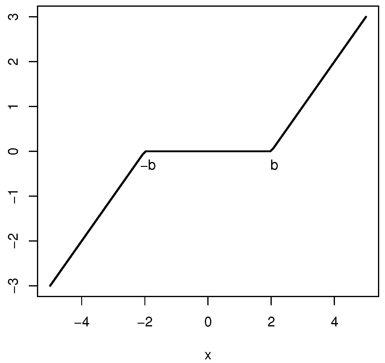
As the classical method-of-moments estimator is the M-estimator associated with the score function and the Huber spatio-temporal variogram estimator, is the M-estimator associated with the score function , where b is the tuning constant, to evaluate the effect of contamination, we define the Difference M-estimator as a solution of the equation
where the score function in (12) is defined as , which is plotted in Figure 8.
The Difference M-estimator, completely defined from (12) as a general M-estimator, can be also considered as the difference of the Average M-estimators associated with the mean and the Huber estimator.
As it is an M-estimator, we can use the VOM + SAD approximation (8) for its distribution obtained above, , with being the score function.
As and are sums of squares, and the latter is softer than the former, we should check for large positive values of the Difference M-estimator as spatio-temporal outliers. Hence, if the probability for a pair of lags (where is the observed value of the Difference M-estimator), is significantly small, we conclude that is a spatio-temporal outlier.
Example 1.
Continuing with the example of Section 7, some of the differences between the classical spatio-temporal estimator and the Huber spatio-temporal estimator are small (e.g., 0.0000 and 0.0299), while others are large (e.g., 6.4689 and 6.6959). With the approximation of the Difference M-estimator, we obtain a table of tail probabilities (i.e., p-values for the test of significant differences), thus, allowing for the detection of spatio-temporal outliers.
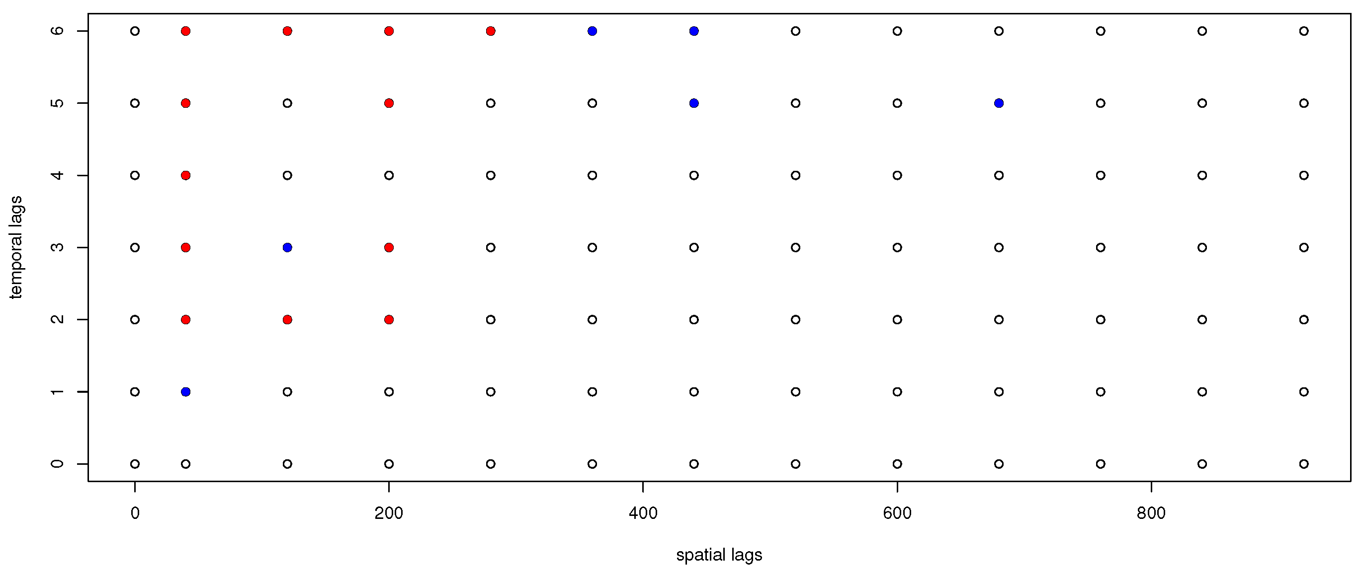
The full table for the 91 pairs of lags considered in this paper is provided in the Supplementary Material. All 91 lags are shown in Figure 9 together with the highly significant spatio-temporal outliers (in red) and the doubtfully significant outliers (in blue).
From the figure, if we discard the doubtful outliers (in blue), we can conclude that some of spatio-temporal lag outliers are essentially only spatial outliers (at from the second temporal lag), while two of them are essentially only temporal outliers (, from the distance lags to ; maybe ). The truly spatio-temporal outliers, in both components, are the intersection lags
We remark that these spatio-temporal outliers are lag outliers (i.e., not observation coordinates); that is, they are outliers with respect to the variogram, where the observations are not the initial but the transformed . Nevertheless, they must be checked before kriging.
10. Conclusions
In this paper, we proposed some robust estimators of the spatio-temporal variogram. We also obtained accurate approximations for their distributions. These were based on a von Mises expansion of the tail probability functional plus a saddlepoint approximation of the Tail Area Influence Function involved in the von Mises expansion. One of the advantages of these approximations is that they have a closed form, thus, allowing for easy interpretation of the elements that they involve, such as the sample size, contamination fraction, score function, temporal and spatial lags and so on.
These approximations are computed under a scale-contaminated normal model for the observations. One of the key points in obtaining these approximations is the transformation of the original variables into new independent variables. With the approximations obtained in this way, we can check, for instance, whether the common use of all the observations without temporal distinctions is valid or if the estimators must be computed for significantly different times. We also used these approximations to identify spatio-temporal outliers in the second part of the paper, defining a new class of M-estimators in the process.
Supplementary Materials
The following supporting information can be downloaded at: https://www.mdpi.com/article/10.3390/math10101785/s1.
Funding
This work was partially supported by grant PGC2018-095194-B-I00 from the Ministerio de Ciencia, Innovación y Universidades (Spain).
Institutional Review Board Statement
Not applicable.
Informed Consent Statement
Not applicable.
Data Availability Statement
Not applicable.
Acknowledgments
The author is very grateful to the referees for their kind and professional remarks.
Conflicts of Interest
The author declares no conflict of interest.
References
- Christakos, G. Spatiotemporal Random Fields: Theory and Applications, 2nd ed.; Elsevier: Amsterdam, The Netherlands, 2017. [Google Scholar]
- Hristopulos, D.T. Random Fields for Spatial Data Modeling: A Primer for Scientists and Engineers; Springer Nature: Berlin, Germany, 2020. [Google Scholar]
- Cressie, N.A.C. Statistics for Spatial Data; John Wiley & Sons: New York, NY, USA, 1993. [Google Scholar]
- Chilès, J.P.; Delfiner, P. Geostatistics: Modeling Spatial Uncertainty, 2nd ed.; John Wiley & Sons: New York, NY, USA, 2012. [Google Scholar]
- Wikle, C.K.; Zammit-Mangion, A.; Cressie, N. Spatio-Temporal Statistics with R; Chapman & Hall/CRC: London, UK, 2019. [Google Scholar]
- Varouchakis, E.A.; Hristopulos, D.T. Comparison of spatiotemporal variogram functions based on a sparse dataset of groundwater level variations. Spat. Stat. 2019, 34, 1–18. [Google Scholar] [CrossRef]
- García-Pérez, A. Saddlepoint approximations for the distribution of some robust estimators of the variogram. Metrika 2020, 83, 69–91. [Google Scholar] [CrossRef]
- García-Pérez, A. New robust cross-variogram estimators and approximations for their distributions based on saddlepoint techniques. Mathematics 2021, 9, 762. [Google Scholar] [CrossRef]
- Huber, P.J.; Ronchetti, E.M. Robust Statistics, 2nd ed.; John Wiley & Sons: New York, NY, USA, 2009. [Google Scholar]
- Tukey, J.W. A survey of sampling from contaminated distributions. In Contributions to Probability and Statistics: Essays in Honor of Harold Hotelling, Stanford Studies in Mathematics and Statistics; Oklin, I., Ed.; Stanford University Press: Redwood City, CA, USA, 1960; Chaper 39; pp. 448–485. [Google Scholar]
- Huber, P.J. Robust estimation of a location parameter. Ann. Math. Stat. 1964, 35, 73–101. [Google Scholar] [CrossRef]
- Ebner, B.; Henze, N. Tests for multivariate normality—A critical review with emphasis on weighted L2-statistics. Test 2020, 29, 845–892. [Google Scholar] [CrossRef]
- Kotz, S.; Balakrishnan, N.; Johnson, N.L. Continuous Multivariate Distributions. Volume 1: Models and Applications, 2nd ed.; John Wiley & Sons: New York, NY, USA, 2000. [Google Scholar]
- Hampel, F.R.; Ronchetti, E.M.; Rousseeuw, P.J.; Syahel, W.A. Robust Statistics: The Approach Based on Influence Functions; John Wiley & Sons: New York, NY, USA, 1986. [Google Scholar]
- Ronchetti, E. Accurate and robust inference. Econom. Stat. 2020, 14, 74–88. [Google Scholar] [CrossRef]
- Cressie, N.; Hawkins, D.M. Robust estimation of the variogram: I. Math. Geol. 1980, 12, 115–125. [Google Scholar] [CrossRef]
- La Vecchia, D.; Ronchetti, E. Saddlepoint approximations for short and long memory time series: A frequency domain approach. J. Econom. 2019, 213, 578–592. [Google Scholar] [CrossRef]
- Von Mises, R. On the asymptotic distribution of differentiable statistical functions. Ann. Math. Stat. 1947, 18, 309–348. [Google Scholar] [CrossRef]
- Withers, C.S. Expansions for the distribution and quantiles of a regular functional of the empirical distribution with applications to nonparametric confidence intervals. Ann. Stat. 1983, 11, 577–587. [Google Scholar] [CrossRef]
- Serfling, R.J. Approximation Theorems of Mathematical Statistics; John Wiley & Sons: New York, NY, USA, 1980. [Google Scholar]
- Field, C.A.; Ronchetti, E. A tail area influence function and its application to testing. Sequential Anal. 1985, 4, 19–41. [Google Scholar] [CrossRef]
- Daniels, H.E. Saddlepoint approximations for estimating equations. Biometrika 1983, 70, 89–96. [Google Scholar] [CrossRef]
- Lugannani, R.; Rice, S. Saddle point approximation for the distribution of the sum of independent random variables. Adv. Appl. Probab. 1980, 12, 475–490. [Google Scholar] [CrossRef]
- García-Pérez, A. Von Mises approximation of the critical value of a test. Test 2003, 12, 385–411. [Google Scholar] [CrossRef]
- Jensen, J.L. Saddlepoint Approximations; Clarendon Press: Oxford, UK, 1995. [Google Scholar]
- R Development Core Team. A Language and Environment for Statistical Computing; R Foundation for Statistical Computing: Viena, Austria, 2021; Available online: http://www.R-project.org (accessed on 18 April 2022).
Figure 1.
Exact and approximate tail probabilities for the empirical spatio-temporal estimator with .
Figure 1.
Exact and approximate tail probabilities for the empirical spatio-temporal estimator with .
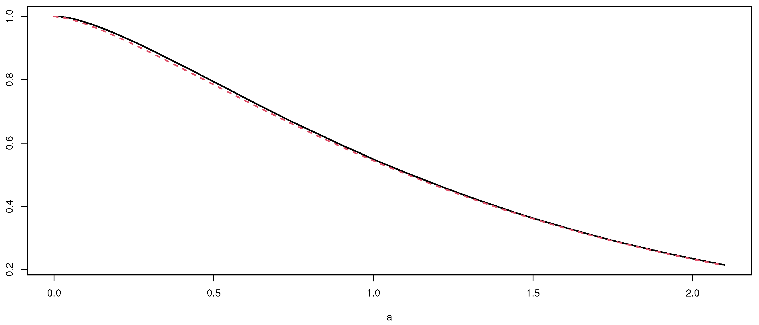
Figure 2.
Exact and approximate tail probabilities of the empirical spatio-temporal estimator with contamination , , and , with sample size .
Figure 2.
Exact and approximate tail probabilities of the empirical spatio-temporal estimator with contamination , , and , with sample size .
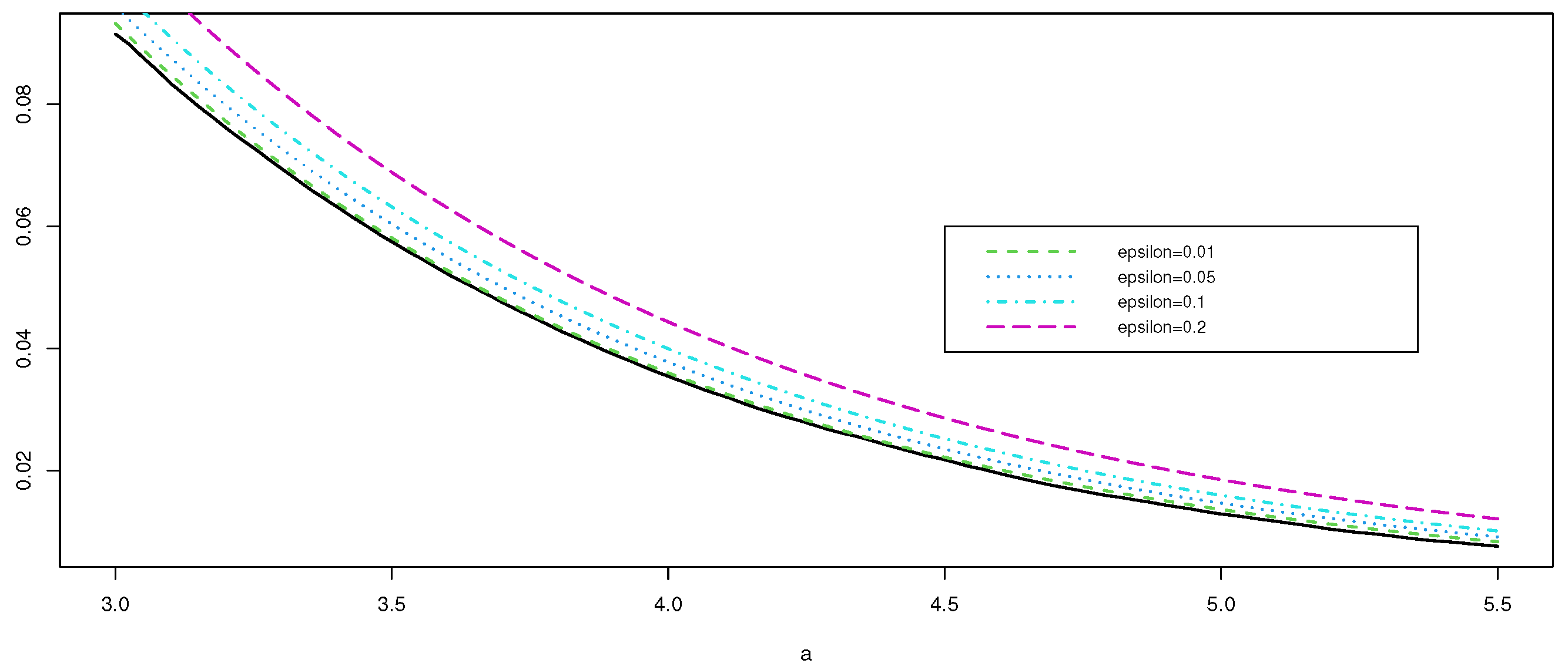
Figure 3.
Huber’s spatio-temporal semivariogram estimator (with tuning constant equal to 1.345) of daily Tmax from the NOAA data set for July 2003, computed using the estimator introduced in Section 6.
Figure 3.
Huber’s spatio-temporal semivariogram estimator (with tuning constant equal to 1.345) of daily Tmax from the NOAA data set for July 2003, computed using the estimator introduced in Section 6.
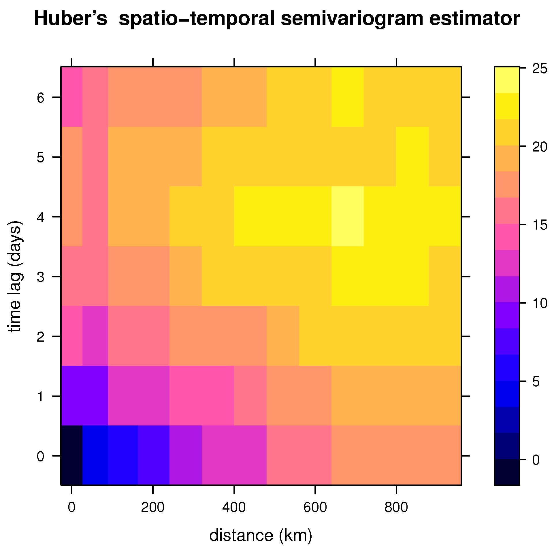
Figure 4.
Three-dimensional picture of the classical spatio-temporal semivariogram estimator of the daily Tmax from the NOAA data for July 2003.
Figure 4.
Three-dimensional picture of the classical spatio-temporal semivariogram estimator of the daily Tmax from the NOAA data for July 2003.
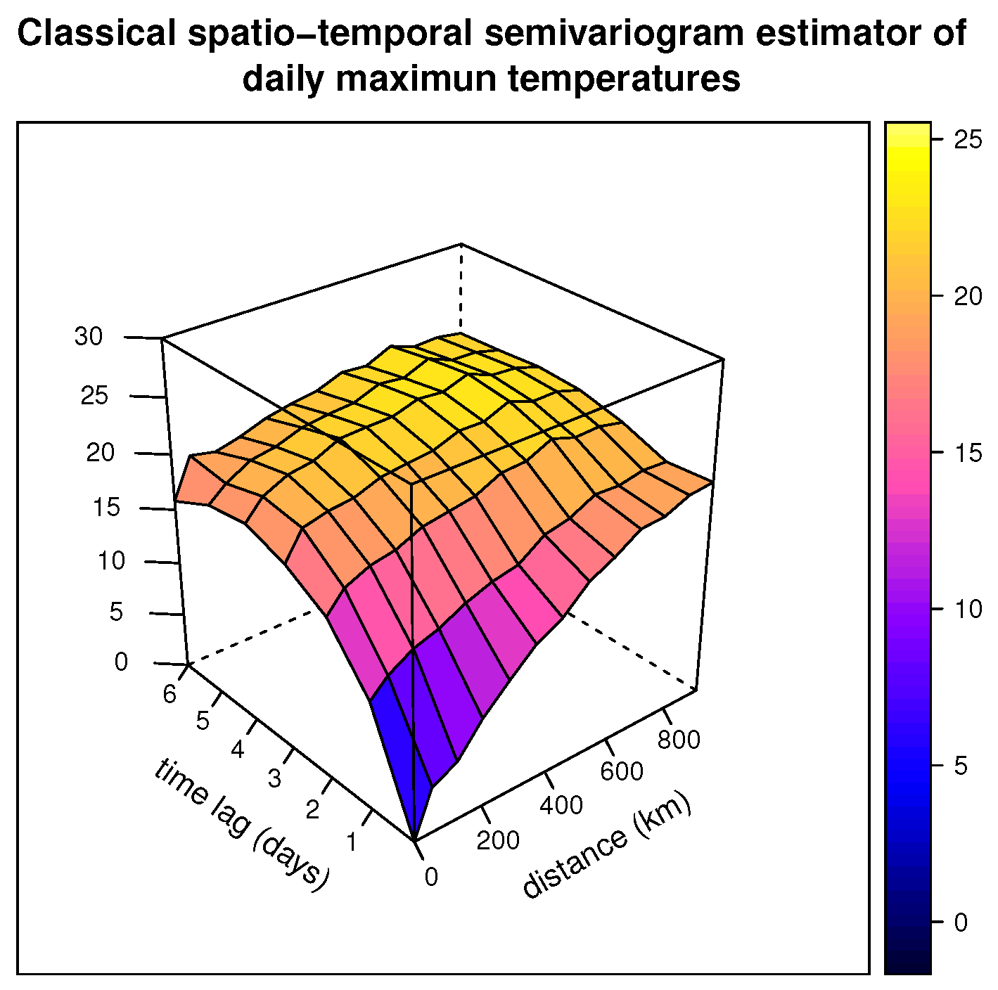
Figure 5.
Three-dimensional picture of the Huber spatio-temporal semivariogram estimator (with a tuning constant equal to 1.345) of the daily Tmax from the NOAA data for July 2003 computed using the estimator introduced in Section 6.
Figure 5.
Three-dimensional picture of the Huber spatio-temporal semivariogram estimator (with a tuning constant equal to 1.345) of the daily Tmax from the NOAA data for July 2003 computed using the estimator introduced in Section 6.

Figure 6.
Classical semivariograms of the daily Tmax from the NOAA data with respect to the seven time lags considered.
Figure 6.
Classical semivariograms of the daily Tmax from the NOAA data with respect to the seven time lags considered.
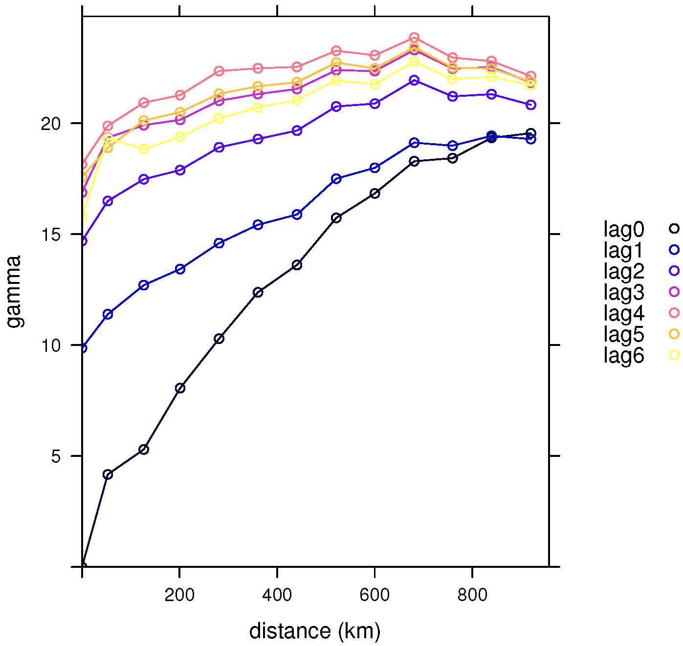
Figure 7.
Huber’s semivariograms (with tuning constant equal to 1.345) of the daily Tmax from the NOAA data with respect to the seven time lags considered.
Figure 7.
Huber’s semivariograms (with tuning constant equal to 1.345) of the daily Tmax from the NOAA data with respect to the seven time lags considered.

Figure 8.
Score function defining the Difference M-estimator with tuning constant b.

Figure 9.
Highly significant spatio-temporal atypical lags (in red) and doubtfully significant (in blue) of the daily Tmax from the NOAA data.
Figure 9.
Highly significant spatio-temporal atypical lags (in red) and doubtfully significant (in blue) of the daily Tmax from the NOAA data.


Table 1.
Tail probabilities for several values of a and sample size .
| a | Exact | Approximation |
|---|---|---|
| 2.5 | 0.14714 | 0.148299 |
| 3.0 | 0.09308 | 0.093233 |
| 3.5 | 0.05577 | 0.058124 |
| 4.0 | 0.03548 | 0.036006 |
| 4.5 | 0.02089 | 0.022196 |
| 5.0 | 0.01313 | 0.013633 |
Publisher’s Note: MDPI stays neutral with regard to jurisdictional claims in published maps and institutional affiliations. |
© 2022 by the author. Licensee MDPI, Basel, Switzerland. This article is an open access article distributed under the terms and conditions of the Creative Commons Attribution (CC BY) license (https://creativecommons.org/licenses/by/4.0/).
Share and Cite
MDPI and ACS Style
García-Pérez, A. On Robustness for Spatio-Temporal Data. Mathematics 2022, 10, 1785. https://doi.org/10.3390/math10101785
AMA Style
García-Pérez A. On Robustness for Spatio-Temporal Data. Mathematics. 2022; 10(10):1785. https://doi.org/10.3390/math10101785
Chicago/Turabian StyleGarcía-Pérez, Alfonso. 2022. "On Robustness for Spatio-Temporal Data" Mathematics 10, no. 10: 1785. https://doi.org/10.3390/math10101785
Note that from the first issue of 2016, this journal uses article numbers instead of page numbers. See further details here.