Stability and Numerical Simulations of a New SVIR Model with Two Delays on COVID-19 Booster Vaccination

Abstract

As COVID-19 continues to threaten public health around the world, research on specific vaccines has been underway. In this paper, we establish an SVIR model on booster vaccination with two time delays. The time delays represent the time of booster vaccination and the time of booster vaccine invalidation, respectively. Second, we investigate the impact of delay on the stability of non-negative equilibria for the model by considering the duration of the vaccine, and the system undergoes Hopf bifurcation when the duration of the vaccine passes through some critical values. We obtain the normal form of Hopf bifurcation by applying the multiple time scales method. Then, we study the model with two delays and show the conditions under which the nontrivial equilibria are locally asymptotically stable. Finally, through analysis of official data, we select two groups of parameters to simulate the actual epidemic situation of countries with low vaccination rates and countries with high vaccination rates. On this basis, we select the third group of parameters to simulate the ideal situation in which the epidemic can be well controlled. Through comparative analysis of the numerical simulations, we concluded that the most appropriate time for vaccination is to vaccinate with the booster shot 6 months after the basic vaccine. The priority for countries with low vaccination rates is to increase vaccination rates; otherwise, outbreaks will continue. Countries with high vaccination rates need to develop more effective vaccines while maintaining their coverage rates. When the vaccine lasts longer and the failure rate is lower, the epidemic can be well controlled within 20 years.

1. Introduction

1.1. Research Background

At present, the Coronavirus Disease 2019 (COVID-19) epidemic has not been completely controlled. The virus (SARS-CoV-2) is highly contagious, spreads by a wide range of routes, and constantly mutates as it spreads, making COVID-19 difficult to control [1]. Since there is no specific treatment for COVID-19, promoting a scale-up of vaccination and building herd immunity is the most effective measure to control the epidemic.

It has always been a hot topic to study the impact of vaccines on the spread of infectious diseases by analyzing the dynamic characteristics of the system [2,3,4,5,6,7]. Among them, De la Sen et al. [4] and Thater et al. [5] proposed different SEIR models of disease transmission for vaccination and developed optimal vaccination strategies. Scherer et al. [6] calculated the threshold vaccination rate to eradicate an infection, and they explored the impact of vaccine-induced immunity that diminishes over time. Many researchers also considered vaccines in their models of COVID-19 epidemics. For example, Yang et al. [8] studied vaccination control in an epidemic model with time delay and applied it to COVID-19. These studies all have shown that vaccination has a significant effect on the control of diseases.

However, the level of neutralizing antibodies decreases over time, and the protective effect of the vaccine diminishes, which also needs to be considered in the model of COVID-19. For example, the SVIR model developed by Duan et al. [9] takes into account that vaccines lose their protective properties over time, allowing vaccinated individuals to become susceptible again. Wald et al. [10] suggest it is necessary to reduce SARS-CoV-2 transmission and infection through enhanced vaccination. This suggests that an additional vaccination regime, called booster immunization, is needed to restore immunity in previously vaccinated populations. Salvagno et al. [11] found a significant decrease in antibodies 6 months after basic vaccination, which is consistent with the need for a vaccine booster. However, few studies have considered the COVID-19 booster vaccine in mathematical models, so we believe that dynamic analysis of the impact of the COVID-19 booster vaccine on epidemic control is needed at present.

There is always a considerable difference between the actual behavior of disease and the response of its mathematical model. In 1979, Cooke proposed the theory of “time delay” in his study of infectious disease transmission, which made the model more realistic [12]. Since then, many researchers have tried to take time delays into account in their models. Zhai et al. [13] studied studies a SEIR epidemic model with time delay and vaccination control. In the infectious disease model for COVID-19, many studies consider a single time delay. For example, Rong et al. [14] studied the effect of delay in diagnosis on the transmission of COVID-19.

Much research shows two delays can reflect the actual problem more clearly. For instance, Song et al. [15] studied a new SVEIRS infectious disease model with pulse and two time delays. In the study of Jiang et al. [16], a SVEIRS epidemic model with two time delays and a nonlinear incidence rate was developed, and they analyzed the dynamic behavior of the model under pulse vaccination. An SEIR epidemic model with two time delays and pulse vaccination was formulated in the study of Gao et al. [17]. However, there are few infectious disease models studying the novel coronavirus that consider two delays. Considering the characteristics of COVID-19 and vaccination, we believe that two time delays can better solve the problems existing in the actual COVID-19 epidemic; that is, we need to give booster shots at intervals after the basic vaccination and take into account the fact that the vaccine does not provide permanent immunity and will lose effectiveness some time after vaccination. Therefore, there are two time delays which cannot be ignored.

The stability of epidemic models and Hopf bifurcation analysis have always been the focus of this kind of epidemic model. In ref [18], Zhang et al. analyzed the stability and Hopf bifurcation of an SVEIR epidemic model with vaccination and multiple time delays. The paper [19] written by Chen et al. mainly addressed stability analysis and estimation of the domain of attraction for the endemic equilibrium of a class of susceptible–exposed–infected–quarantine epidemic models. Li et al. [20] studied the stability and bifurcation analysis of an SIR epidemic model with logistic growth and saturation processing. In the study of Goel et al. [21], a time-delayed SIR epidemic model with a logistic growth of susceptibles was proposed and analyzed mathematically. The stability behavior of the model was analyzed for two equilibria: the disease-free equilibrium and the endemic equilibrium. Further, they investigated the stability behavior, demonstrating the occurrence of oscillatory and periodic solutions through Hopf bifurcation concerning every possible grouping of two time delays as the bifurcation parameter.

1.2. Research Motivation

The research motivation of this paper is as follows. There have been mass vaccine injections worldwide, but the level of antibodies in the receptor decreases over time, and the protective effect of the vaccine diminishes, so we also need to strengthen immunity to enhance the body’s ability to resist SARS-CoV-2. In such cases, increasing the number of vaccinations is a measure to improve the level of immunity and increase protection. Therefore, the booster shot we are considering is a dose of vaccine that is administered again after the completion of the COVID-19 vaccine by antibody resolution in order to maintain immunity to COVID-19. Currently, the third dose of inactivated COVID-19 vaccine is the main booster vaccination in the world. The first and second doses of the COVID-19 vaccine are commonly referred to as basic vaccines. If the basic vaccine protection effect is still good, early booster vaccination wastes resources; if the interval between booster vaccination and basic vaccination is too long, it can cause the failure of herd immunity, and the epidemic will be out of control.

Thus, we first want to study the most appropriate time to give a booster vaccine. Therefore, we create a mathematical model that takes into account both basic and booster vaccination. Second, since the efficacy of the vaccine is unknown, we also consider the effect of the duration of the booster vaccine on the timing of the booster vaccination. We aim to develop a vaccine approach that can effectively help control the COVID-19 epidemic through dynamic analysis of the model that takes these two time delays into account. Third, different countries have different vaccine coverage rates and levels of concern. Our goal is to select different parameter groups to simulate the epidemic in different countries and to give the vaccination time requirements for epidemic control. At the same time, we select a set of ideal parameters that represent that the epidemic can be well controlled and compare them to the actual parameters to study what efforts we still need to make at present.

The structure of this paper is as follows. In Section 2, we establish an SVIR booster vaccination model with two time delays. In Section 3, we analyze the existence and stability of non-negative equilibria and discuss the existence of Hopf bifurcation. We deduce the normal form of Hopf bifurcation in Section 4. In Section 5, we give some numerical simulations and get the conclusion of strengthening inoculation time. Finally, conclusions and suggestions are given in Section 6.

2. Mathematical Modeling

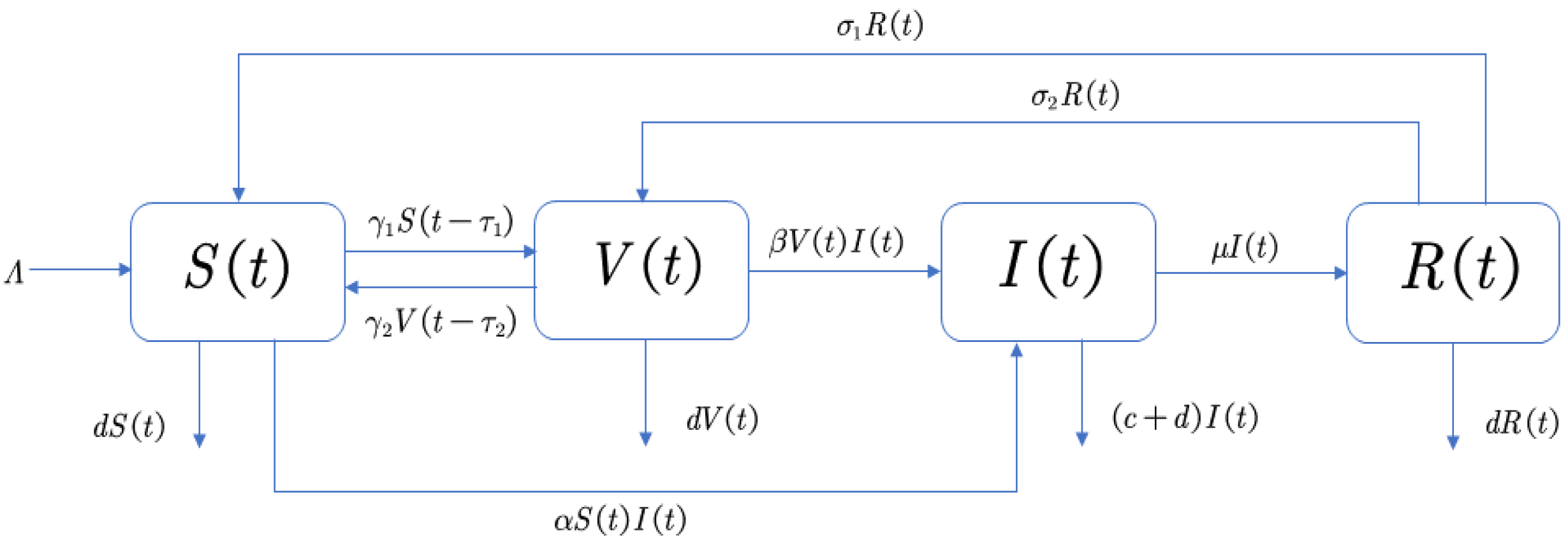
Different from the traditional infectious disease model, we redefined the cabin so that our model could better depict the relationship between basic vaccination and booster vaccination in order to study the role of booster vaccine in epidemic control. We divided COVID-19 susceptible people into two groups. One group involves people who have received basic but not booster shots (S), and the other group involves people who have completed all vaccinations (V); both groups are at risk of contracting COVID-19 through contact with infected people or other means and becoming infected (I). However, it should be noted that the infection rate of the susceptible in V is much lower than that of the susceptible in S. Some of the infected I will die of the disease, while others will recover (R) after treatment. However, their vaccine will be ineffective to varying degrees according to their conditions [22]. For people such as the elderly or those with underlying diseases who have recovered, the antibodies produced by the vaccine are almost completely disabled, and they need a basic injection to regain active antibodies. This group of people will become S. Otherwise, people who maintain some antibody activity in their bodies just need a booster shot to increase their resistance to SARS-CoV-2. They become V.

Taking all these factors into account, we get the concrete conversion between the four cabins shown in Figure 1.

Table 1. Description of variables and parameters in the model.

Symbol	Description
S	Number of susceptible persons who have received basic but not booster shots
V	Number of susceptible persons who have completed all vaccinations
I	Number of patients affected
R	Number of recovered persons
$\Lambda$	Inoculation rate of basic vaccine
$\alpha$	Transition rate from S to I
$\beta$	Transition rate from V to I
${\gamma }_1$	Transition rate from S to V
${\gamma }_2$	Transition rate from V to S
$\mu$	Transition rate from I to R; the cure rate of infected persons
${\sigma }_1$	Transition rate from R to S
${\sigma }_2$	Transition rate from R to V
c	National case fatality rate of COVID-19
d	Natural death rate of population
${\tau }_1$	Time-delay for people who received the basic vaccine to receive the booster vaccine
${\tau }_2$	Time-delay from people getting booster vaccination to their antibodies disappearing

shows specific definitions of variables and parameters. In this table, all parameters and variables are positive.

For COVID-19 vaccines, susceptible people develop antibodies after vaccination, but the vaccine cannot provide long-term protection according to the background in Section 1.1. We assume that in our model, the basic vaccine’s activity declines over time, but will become ineffective only if a person gets sick. Since the booster vaccine is only a supplement to the basic vaccine, the dose is less than the basic vaccine. We assume that over a long period, the potency of the antibody produced by the booster vaccine will gradually decline until it disappears. We define the time delay of the booster vaccine’s failure in our model as ${\tau }_2$. At the same time, as considered in Section 1.2, to keep the epidemic under control and to maximize the use of resources, those who receive only the basic vaccine need to receive booster shots after a certain time delay, as indicated by ${\tau }_1$. In general, the duration of the vaccine’s effective protection must be longer than the interval between vaccinations, so we specify ${\tau }_2>{\tau }_1$ in our model. Therefore, we construct the following differential equation:

$$\left\{\begin{array}{cc}\hfill \frac{dS\left(t\right)}{dt}=& \Lambda -{\gamma }_{1}S\left(t-{\tau }_1\right)+{\gamma }_{2}V\left(t-{\tau }_2\right)-\alpha S\left(t\right)I\left(t\right)+{\sigma }_{1}R\left(t\right)-dS\left(t\right),\hfill \\ \hfill \frac{dV\left(t\right)}{dt}=& {\gamma }_{1}S\left(t-{\tau }_1\right)-{\gamma }_{2}V\left(t-{\tau }_2\right)-\beta V\left(t\right)I\left(t\right)+{\sigma }_{2}R\left(t\right)-dV\left(t\right),\hfill \\ \hfill \frac{dI\left(t\right)}{dt}=& \alpha S\left(t\right)I\left(t\right)+\beta V\left(t\right)I\left(t\right)-\mu I\left(t\right)-\left(c+d\right)I\left(t\right),\hfill \\ \hfill \frac{dR\left(t\right)}{dt}=& \mu I\left(t\right)-{\sigma }_{1}R\left(t\right)-{\sigma }_{2}R\left(t\right)-dR\left(t\right).\hfill \end{array}\right.$$

(1)

The meanings of variables and parameters are given in Table 1. Timely booster vaccinations prevent inadequate antibody levels in individuals, which could lead to increased infection rates and the situation of the epidemic being out of control. Therefore, it is particularly important to choose the right timing for booster vaccination to control the epidemic.

3. Stability Analysis of Equilibria and Existence of Hopf Bifurcation

In this section, System (1) is considered. Obviously, System (1) has three equilibria:

$$\begin{array}{c}\hfill E_1=\left(S_1,V_1,0,0\right),E_{2_l}=\left(S_{2_l},V_{2_l},I_{2_l},R_{2_l}\right),l=1,2\end{array}$$

(2)

where $S_1=\frac{\Lambda }{{\gamma }_1-\xi +d},V_1=\frac{\xi \Lambda }{\left({\gamma }_1-\xi +d\right){\gamma }_2},$ with $\xi =\frac{{\gamma }_1{\gamma }_2}{{\gamma }_2+d}$, and $R_{2_1}=\frac{-{\Gamma }_1-\sqrt{{\Gamma }_2^2-4{\Gamma }_1{\Gamma }_3}}{2{\Gamma }_1},R_{2_2}=\frac{-{\Gamma }_1+\sqrt{{\Gamma }_2^2-4{\Gamma }_1{\Gamma }_3}}{2{\Gamma }_1},S_{2_l}=b-ef-eg{R}_{2_l},V_{2_l}=f+g{R}_{2_l},I_{2_l}=a{R}_{2_l}$, with $a=\frac{{\sigma }_1+{\sigma }_2+d}{\mu }$, $b=\frac{\mu +c+d}{\alpha }$, $e=\frac{\beta }{\alpha }$, $f=\frac{\Lambda -bd}{d-ed}$, $g=\frac{\mu d+\left(c+d\right)\left({\sigma }_1+{\sigma }_2+d\right)}{\mu \left(ed-d\right)}$, ${\Gamma }_1=\beta ag$, ${\Gamma }_2=dg-{\sigma }_2+\beta fa+{\gamma }_{2}g+eg{\gamma }_1$, ${\Gamma }_3=df+{\gamma }_2-{\gamma }_1\left(b-ef\right)$.

For equilibria $E_1,E_{2_l}$, we consider the following assumption:

Hypothesis 1 (H1). 

${\gamma }_1-\xi +d>0$.

When (H1) holds, the equilibrium $E_1$ exists and is non-negative.

Hypothesis 2 (H2). 

${\Gamma }_1<0,{\Gamma }_2>0,{\Gamma }_3<0$ or ${\Gamma }_1<0,{\Gamma }_2>0,{\Gamma }_3>0$.

When (H2) holds, the equilibrium $E_{2_1}$ exists and is positive.

Hypothesis 3 (H3). 

${\Gamma }_1<0,{\Gamma }_2>0,{\Gamma }_3<0$ or ${\Gamma }_1<0,{\Gamma }_2<0,{\Gamma }_3>0$.

When (H3) holds, the equilibrium $E_{2_2}$ exists and is positive. We calculate the basic reproduction number $R_0$, the number of the suspected individuals who are infected by the same infectious individual, and can estimate the infectiousness of an infectious disease. According to System (1), we can get the new infections matrix $\mathcal{F}$ and the transition matrix $\mathcal{V}$.

$$\mathcal{F}=\left[\begin{array}{c}0\\ 0\\ \alpha S\left(t\right)I\left(t\right)+\beta V\left(t\right)I\left(t\right)\\ 0\end{array}\right],\mathcal{V}=\left[\begin{array}{c}-\Lambda +{\gamma }_{1}S\left(t\right)-{\gamma }_{2}V\left(t\right)-{\sigma }_{1}R\left(t\right)+dS\left(t\right)+\alpha S\left(t\right)I\left(t\right)\\ -{\gamma }_{1}S\left(t\right)+{\gamma }_{2}V\left(t\right)+\beta V\left(t\right)I\left(t\right)-{\sigma }_{2}R\left(t\right)+dV\left(t\right)\\ \mu I\left(t\right)+cI\left(t\right)+dI\left(t\right)\\ -\mu I\left(t\right)+{\sigma }_{1}R\left(t\right)+{\sigma }_{2}R\left(t\right)+dR\left(t\right)\end{array}\right].$$

Then, we make $F_0$ represent the derivative of $\mathcal{F}$ at $E_1$ and $V_0$ represent the derivative of $\mathcal{V}$ at $E_1$:

$$F_0=\left[\begin{array}{cccc}0& 0& 0& 0\\ 0& 0& 0& 0\\ 0& 0& \alpha S_1+\beta V_1& 0\\ 0& 0& 0& 0\end{array}\right],V_0=\left[\begin{array}{cccc}{\gamma }_1+d& -{\gamma }_2& \alpha S_1& -\sigma {}_1\\ -{\gamma }_1& {\gamma }_2+d& \beta V_1& -\sigma {}_2\\ 0& -\epsilon & \mu +c+d& 0\\ 0& -{\gamma }_1& -\mu & {\sigma }_1+{\sigma }_2+d\end{array}\right].$$

We can obtain:

$$F_0{V}_0^{-1}=\left[\begin{array}{cccc}0& 0& 0& 0\\ 0& 0& 0& 0\\ 0& 0& \frac{\alpha S_1+\beta V_1}{\mu +c+d}& 0\\ 0& 0& 0& 0\end{array}\right].$$

The maximum eigenvalue of $F_0{V}_0^{-1}$ is the basic regeneration number of System (1):

$$R_0=\rho \left(F_0{V}_0^{-1}\right)=\frac{\alpha S_1+\beta V_1}{\mu +c+d}.$$

Transferring the equilibria $E_k,(k=1,2_1,2_2)$ to the origin point: $\tilde{S}=S-S_k$, $\tilde{V}=V-V_k$, $\tilde{I}=I-I_k$, $\tilde{R}=R-R_k$ and linearizing System (1) around them. Renewedly denoting $\tilde{S},\tilde{V},\tilde{I},\tilde{R}$ as $S,V,I,R$, we obtain the following model:

$$\left\{\begin{array}{cc}\hfill \frac{dS}{dt}=& -{\gamma }_{1}S\left(t-{\tau }_1\right)+{\gamma }_{2}V\left(t-{\tau }_2\right)-\alpha SI+{\sigma }_{1}R-dS-\alpha S_{k}I-\alpha S{I}_k,\hfill \\ \hfill \frac{dV}{dt}=& {\gamma }_{1}S\left(t-{\tau }_1\right)-{\gamma }_{2}V\left(t-{\tau }_2\right)-\beta VI-\beta V_{k}I-\beta V{I}_k+{\sigma }_{2}R-dV,\hfill \\ \hfill \frac{dI}{dt}=& \alpha SI+\alpha S_{k}I+\alpha S{I}_k+\beta VI+\beta V_{k}I+\beta V{I}_k-\mu I-\left(c+d\right)I,\hfill \\ \hfill \frac{dR}{dt}=& \mu I-{\sigma }_{1}R-{\sigma }_{2}R-dR.\hfill \end{array}\right.$$

(3)

We can get the characteristic equation of the linearized system (1) as follows:

$$\begin{array}{c}\hfill {\sigma }_1{\mathrm{e}}^{-\lambda {\tau }_1}\left({\lambda }^3+B_1{\lambda }^2+C_1\lambda +D_1\right)+{\sigma }_2{\mathrm{e}}^{-\lambda {\tau }_2}\left({\lambda }^3+B_2{\lambda }^2+C_2\lambda +D_2\right)\\ \hfill +{\lambda }^4+A_3{\lambda }^3+B_3{\lambda }^2+C_3\lambda +D_3=0,\end{array}$$

(4)

where

$$\begin{array}{c}\hfill \begin{array}{cc}\hfill & \begin{array}{cc}& B_1={\sigma }_1+{\sigma }_2+3d+\mu +c+\beta I_k-\alpha S_k-\beta V_k,\hfill \end{array}\hfill \\ \hfill & \begin{array}{cc}& C_1=\left({\sigma }_1+{\sigma }_2+d\right)\left(2d+\mu +c+\beta I_k-\alpha S_k-\beta V_k\right)+\left(d+\mu +c\right)\beta I_k+d\left(d+\mu +c-\alpha S_k-\beta V_k\right),\hfill \end{array}\hfill \\ \hfill & \begin{array}{cc}& D_1=\left({\sigma }_1+{\sigma }_2+d\right)\left[\left(d+\mu +c\right)\beta I_k+d\left(d+\mu +c-\alpha S_k-\beta V_k\right)-\mu {\sigma }_1\beta I_k-\mu {\sigma }_2\beta I_k\right],\hfill \end{array}\hfill \\ \hfill & \begin{array}{cc}& B_2={\sigma }_1+{\sigma }_2+3d+\mu +c+\alpha I_k-\alpha S_k-\beta V_k,\hfill \end{array}\hfill \\ \hfill & \begin{array}{cc}& C_2=\left({\sigma }_1+{\sigma }_2+d\right)\left(2d+\mu +c+\alpha I_k-\alpha S_k-\beta V_k\right)+d\left(d+\mu +c-\alpha S_k-\beta V_k\right)+\left(d+\mu +c\right)\alpha I_k,\hfill \end{array}\hfill \\ \hfill & \begin{array}{cc}& D_2=\left({\sigma }_1+{\sigma }_2+d\right)\left[\left(d+\mu +c\right)\alpha I_k+d\left(d+\mu +c-\alpha S_k-\beta V_k\right)-\mu {\sigma }_1\alpha I_k-\mu {\sigma }_2\alpha I_k\right],\hfill \end{array}\hfill \\ \hfill & \begin{array}{cc}& A_3={\sigma }_1+{\sigma }_2+4d+\mu +c+\alpha I_k+\beta I_k-\alpha S_k-\beta V_k,\hfill \end{array}\hfill \\ \hfill & \begin{array}{cc}\hfill B_3=& \left({\sigma }_1+{\sigma }_2+d\right)\left(3d+\mu +c+\alpha I_k+\beta I_k-\alpha S_k-\beta V_k\right)+\left[\left(d+\alpha I_k\right)\left(2d+\mu +c+\beta I_k-\alpha S_k-\beta V_k\right)\right.\hfill \\ \hfill & \left.+\left(d+\beta I_k\right)\left(d+\mu +c-\alpha S_k-\beta V_k\right)+{\beta }^2{I}_k{V}_k+{\alpha }^2{I}_k{S}_k\right],\hfill \end{array}\hfill \\ \hfill & \begin{array}{cc}\hfill C_3=& \left({\sigma }_1+{\sigma }_2+d\right)\left[\left(d+\alpha I_k\right)\left(2d+\mu +c+\beta I_k-\alpha S_k-\beta V_k\right)+\left(d+\beta I_k\right)\left(d+\mu +c-\alpha S_k-\beta V_k\right)\right.\hfill \\ \hfill & \left.+{\beta }^2{I}_k{V}_k+{\alpha }^2{I}_k{S}_k\right]+{\alpha }^2{I}_k{S}_k\left(d+\beta I_k\right)-\mu {\sigma }_1\alpha I_k-\mu {\sigma }_2\beta I_k,\hfill \end{array}\hfill \\ \hfill & \begin{array}{cc}& D_3={\alpha }^2{I}_k{S}_k\left(d+\beta I_k\right)\left({\sigma }_1+{\sigma }_2+d\right)-\mu {\sigma }_1\left(\alpha \beta I_k^2+\alpha d{I}_k\right)-\mu {\sigma }_2\left(\alpha \beta I_k^2+\beta d{I}_k\right),k=1,2_1,2_2.\hfill \end{array}\hfill \end{array}\end{array}$$

3.1. Analysis for Disease-Free Equilibrium $E_1$

3.1.1. The Case for ${\tau }_1=0$, ${\tau }_2=0$

Firstly, we consider $R_0<1$. The characteristic equation of the linearized system (1) about $E_1$ is as follows:

$$\left(\lambda +\mu a\right)\left(\lambda +\mu +c+d-\beta V_1-\alpha S_1\right)\left[\left({\left(\lambda +d\right)}^2+\left(\lambda +d\right){\sigma }_1{\mathrm{e}}^{-\lambda {\tau }_1}+\left(\lambda +d\right){\sigma }_2{\mathrm{e}}^{-\lambda {\tau }_2}\right)\right]=0.$$

(5)

When ${\tau }_1=0$, ${\tau }_2=0$, it turns to

$$\left(\lambda +{\sigma }_1+{\sigma }_2+d\right)\left(\lambda +\mu +c+d-\beta V_1-\alpha S_1\right)\left(\lambda +d\right)\left(\lambda +d+{\sigma }_1+{\sigma }_2\right)=0.$$

(6)

Obviously, all the roots of Equation (6) have negative real parts due to $R_0<1,{\sigma }_1>0,{\sigma }_2>0,d>0$. We can conclude the disease-free equilibrium $E_1$ is locally asymptotically stable when ${\tau }_1=0,{\tau }_2=0$.

When $R_0>1$, Equation (6) has a positive root. Thus, the disease-free equilibrium $E_1$ is unstable when ${\tau }_1=0,{\tau }_2=0$.

3.1.2. The Case for ${\tau }_1=0$, ${\tau }_2>0$

When ${\tau }_2>0$, for equilibrium $E_1$, we simply need to think about the following equation

$${\left(\lambda +d\right)}^2+\left(\lambda +d\right){\sigma }_1+\left(\lambda +d\right){\sigma }_2{\mathrm{e}}^{-\lambda {\tau }_2}=0.$$

(7)

To discuss the existence of Hopf bifurcation for $E_1$, we assume that $\lambda =\mathrm{i}{\omega }_1({\omega }_1>0)$ is a pure imaginary root of Equation (7). Substituting it into Equation (7) and separating the real and imaginary parts, we obtain:

$$\left\{\begin{array}{c}{\gamma }_2{\omega }_1\sin \left({\omega }_1{\tau }_2\right)+d{\gamma }_2\cos \left({\omega }_1{\tau }_2\right)={\omega }_1^2-d^2-d{\gamma }_1\hfill \\ d{\gamma }_2\sin \left({\omega }_1{\tau }_2\right)-{\gamma }_2{\omega }_1\cos \left({\omega }_1{\tau }_2\right)={\omega }_1\left(2d+{\gamma }_1\right)\hfill \end{array}\right.$$

(8)

Equation (8) derives to:

$$\left\{\begin{array}{c}\sin \left({\omega }_1{\tau }_2\right)=\frac{{\omega }_1^3-\left(d^2+d{\gamma }_1\right){\omega }_1+\left(2d^2{\gamma }_2+d{\gamma }_1{\gamma }_2\right){\omega }_1}{{\gamma }_2\left({\omega }_1^2+d^2\right)},\hfill \\ \cos \left({\omega }_1{\tau }_2\right)=\frac{-\left(d{\gamma }_2+{\gamma }_1{\gamma }_2\right){\omega }_1^2-d^3{\gamma }_2-d^2{\gamma }_1{\gamma }_2}{{\gamma }_2\left({\omega }_1^2+d^2\right)}.\hfill \end{array}\right.$$

(9)

Adding the square of two equations in Equation (8) and letting $z={\omega }_1^2$, we get

$$\begin{array}{c}\hfill h\left(z\right)=z^2+c_{1}z+c_0=0,\end{array}$$

(10)

where $c_1=\left[{\left(2d+{\gamma }_1\right)}^2-{\gamma }_2^2-2\left(d^2+d{\gamma }_1\right)\right],c_0={\left(d^2+d{\gamma }_1\right)}^2-d^2{\gamma }_2^2$.

Therefore, we show the following assumptions:

Hypothesis 4 (H4).

$c_0<0$;

Hypothesis 5 (H5).

$c_1^2-4c_0>0,c_1<0,c_0>0$;

Hypothesis 6 (H6).

$c_1^2-4c_0<0,c_0>0$ or $c_1^2-4c_0>0,c_1>0,c_0>0$.

Under (H4), Equation (10) has the unique positive root $z_1$. If (H5) holds, Equation (10) has two positive roots: $z_2$ and $z_3(z_2<z_3)$. Under (H6), Equation (10) has no root. Substituting ${\omega }_{1k}=\sqrt{z_k}(k=1,2,3)$ into Equation (9), we get the expression of ${\tau }_2$:

$$\begin{array}{c}\hfill {\tau }_{2k}^{\left(j\right)}=\left\{\begin{array}{cc}\frac{1}{{\omega }_{1k}}[\arccos \left(P_k\right)+2j\pi ],\hfill & Q_k\ge 0,\hfill \\ \frac{1}{{\omega }_{1k}}[2\pi -\arccos \left(P_k\right)+2j\pi ],\hfill & Q_k<0,k=1,2,3j=0,1,2,\cdots ,\hfill \end{array}\right.\end{array}$$

(11)

where $Q_k=\sin \left({\omega }_{1k}{\tau }_{2k}^{\left(j\right)}\right),P_k=\cos \left({\omega }_{1k}{\tau }_{2k}^{\left(j\right)}\right).$

If $R_0<1$, when ${\tau }_2={\tau }_{2k}^{\left(j\right)}(k=1,2,3;j=0,1,2,\cdots )$, then Equation (7) has a pair of pure imaginary roots $\pm \mathrm{i}{\omega }_{1k}$, and all the other roots of Equation (7) have nonzero real parts. Furthermore, let $\lambda \left(\tau \right)=\alpha \left(\tau \right)+\mathrm{i}{\omega }_1\left(\tau \right)$ be the root of Equation (7) satisfying $\alpha \left({\tau }_k^{\left(j\right)}\right)=0$, $\omega \left({\tau }_k^{\left(j\right)}\right)={\omega }_{1k}(k=1,2,3;j=0,1,2,\cdots )$. Thus, $z_k={\omega }_{1k}^2$, $h^{\prime }\left(z_k\right)\ne 0$, where $h^{\prime }\left(z\right)$ is the derivative of $h\left(z\right)$ with respect to z. Then, we have the following transversality condition:

$$\mathrm{Re}\left(\frac{\mathrm{d}\tau }{\mathrm{d}\lambda }\right)\left|{}_{\tau ={\tau }_{2k}^{\left(j\right)}}\right.=\mathrm{Re}{\left(\frac{\mathrm{d}\lambda }{\mathrm{d}\tau }\right)}^{-1}\left|{}_{\tau ={\tau }_{2k}^{\left(j\right)}}\right.=\frac{h^{\prime }\left({\omega }_{1k}^2\right)}{{\gamma }_2^2\left({\omega }_{1k}^2+d^2\right)}\ne 0,k=1,2,3j=0,1,2,\cdots .$$

Lemma 1.

If $R_0<1$ holds, the equilibrium $E_1$ is stable and undergoes Hopf bifurcation at $\tau ={\tau }_{2k}^{\left(j\right)}(k=1,2,3;j=0,1,2,\cdots )$, where ${\tau }_{2k}^{\left(j\right)}$ is given by Equation (11). Further, we denote the stable region of $E_1$ as I.

3.1.3. The Case for ${\tau }_1>0$, ${\tau }_2>0$

With the above analysis, we choose ${\tau }_2={\tau }_{2*}\in$ I as a parameter; the characteristic equation of system (1) is rewritten as follows:

$${\left(\lambda +d\right)}^2+\left(\lambda +d\right){\sigma }_1{\mathrm{e}}^{-\lambda {\tau }_1}+\left(\lambda +d\right){\sigma }_2{\mathrm{e}}^{-\lambda {\tau }_{2*}}=0.$$

Letting $\lambda =\mathrm{i}{\tilde{\omega }}_1(\tilde{\omega }>0)$ be the root of the above equation, then separating the real and imaginary parts for the above equation, we get

$$\left\{\begin{array}{c}{{\tilde{\omega }}_1}^2-d^2-{\gamma }_2{\tilde{\omega }}_1\sin \left({\tilde{\omega }}_1{\tau }_{2*}\right)-d{\gamma }_2\cos \left({\tilde{\omega }}_1{\tau }_{2*}\right)={\gamma }_1{\tilde{\omega }}_1\sin \left({\tilde{\omega }}_1{\tau }_1\right)+d{\gamma }_1\cos \left({\tilde{\omega }}_1{\tau }_1\right),\hfill \\ 2d{\tilde{\omega }}_1-d{\gamma }_2\sin \left({\tilde{\omega }}_1{\tau }_{2*}\right)+{\gamma }_2{\tilde{\omega }}_1\cos \left({\tilde{\omega }}_1{\tau }_{2*}\right)=d{\gamma }_1\sin \left({\tilde{\omega }}_1{\tau }_1\right)-{\gamma }_1{\tilde{\omega }}_1\cos \left({\tilde{\omega }}_1{\tau }_1\right),\hfill \end{array}\right.$$

which leads to

$$\begin{array}{cc}\hfill F_1\left({\tilde{\omega }}_1\right)=& {{\tilde{\omega }}_1}^4+\left(2d^2-{\gamma }_1^2+{\gamma }_2^2\right){{\tilde{\omega }}_1}^2+d^4-d^2{\gamma }_1^2+d^2{\gamma }_2^2\hfill \\ \hfill & -2\left({{\tilde{\omega }}_1}^2-d^2\right)\left[{\gamma }_2\sin \left({\tilde{\omega }}_1{\tau }_{2*)}\right){\tilde{\omega }}_1+d{\gamma }_2\cos \left({\tilde{\omega }}_1{\tau }_{2*}\right)\right]\hfill \\ \hfill & +4d{\tilde{\omega }}_1\left[{\gamma }_2{\tilde{\omega }}_1\cos \left({\tilde{\omega }}_1{\tau }_{2*}\right)-d{\gamma }_2\sin \left({\tilde{\omega }}_1{\tau }_{2*}\right)\right].\hfill \end{array}$$

(12)

Suppose

Hypothesis 7 (H7).

$d^4-2{\gamma }_2{d}^3-\left({\gamma }_1^2-{\gamma }_2^2\right)d^2<0$. Then, we have $F_1\left(0\right)<0$ and $F_1\left(\infty \right)>0$.

Hence, $F_1\left({\tilde{\omega }}_1\right)=0$ has definite positive roots ${\tilde{\omega }}_{1k},k=0,1,2.$ For every fixed ${\tilde{\omega }}_{1k}$, there is a sequence of ${\tau }_1$ defined by:

$$\begin{array}{c}\hfill {\tau }_{1k}^{\left(j\right)}=\left\{\begin{array}{cc}\frac{1}{{\tilde{\omega }}_{1k}}[\arccos \left(P_{1k}\right)+2j\pi ],\hfill & Q_{1k}\ge 0,\hfill \\ \frac{1}{{\tilde{\omega }}_{1k}}[2\pi -\arccos \left(P_{1k}\right)+2j\pi ],\hfill & Q_{1k}<0,k=1,2j=0,1,2,\cdots ,\hfill \end{array}\right.\end{array}$$

(13)

where

$$\left\{\begin{array}{c}{Q}_{1k}\stackrel{\Delta }{=}\sin \left({\tilde{\omega }}_1{\tau }_{1k}^{\left(j\right)}\right)=\frac{{\tilde{\omega }}_1\left[{{\tilde{\omega }}_1}^2-d^2-{\gamma }_2\sin \left({\tilde{\omega }}_1{\tau }_{2*}\right){\tilde{\omega }}_1-d{\gamma }_2\cos \left({\tilde{\omega }}_1{\tau }_{2*}\right)\right]+d\left[2d{\tilde{\omega }}_1+{\gamma }_2{\tilde{\omega }}_1\cos \left({\tilde{\omega }}_1{\tau }_{2*}\right)-d{\gamma }_2\sin \left({\tilde{\omega }}_1{\tau }_{2*}\right)\right]}{{\gamma }_1\left({{\tilde{\omega }}_1}^2+d^2\right)},\hfill \\ P_{1k}\stackrel{\Delta }{=}\cos \left({\tilde{\omega }}_1{\tau }_{1k}^{\left(j\right)}\right)=\frac{d\left[{{\tilde{\omega }}_1}^2-d^2-{\gamma }_2\sin \left({\tilde{\omega }}_1{\tau }_{2*}\right){\tilde{\omega }}_1-d{\gamma }_2\cos \left({\tilde{\omega }}_1{\tau }_{2*}\right)\right]-{\tilde{\omega }}_1\left[2d{\tilde{\omega }}_1+{\gamma }_2{\tilde{\omega }}_1\cos \left({\tilde{\omega }}_1{\tau }_{2*}\right)-d{\gamma }_2\sin \left({\tilde{\omega }}_1{\tau }_{2*}\right)\right]}{{\gamma }_1\left({{\tilde{\omega }}_1}^2+d^2\right)}.\hfill \end{array}\right.$$

Lemma 2.

Let ${\tau }_{1*}=min{\tau }_{1k}^{\left(j\right)},i=0,1,2,j=0,1,2,\cdots ,$ when ${\tau }_1={\tau }_{1*}$, Equation (12) has a pair of purely imaginary roots $\pm \mathrm{i}{\tilde{\omega }}_1$ for ${\tau }_2\in I$. Assume $\mathrm{Re}\left(\frac{\mathrm{d}\tau }{\mathrm{d}\lambda }\right)\left|{}_{\tau ={\tau }_{1k}^{\left(j\right)}}\right.\ne 0$. Thus, the equilibrium $E_1$ is locally asymptotically stable when ${\tau }_1\in \left[\left.0,{\tau }_{1*}\right)\right.$.

Theorem 1.

For equilibrium $E_1$, we have the following conclusions.

When (H1) does not hold or $R_0>1$ holds, equilibrium $E_1$ is unstable; When (H1) and $R_0<1$ hold,

(1) 

${\tau }_1=0,{\tau }_2=0$

Equilibrium $E_1$ is locally asymptotically stable;

(2) 

${\tau }_1=0,{\tau }_2>0$

(a) 

If (H4) holds, $h\left(z\right)$ has only one positive root $z_1$, when ${\tau }_1\in [0,{\tau }_{21}^{\left(0\right)})$, the equilibrium $E_1$ is locally asymptotically stable;

(b) 

If (H5) holds, $h\left(z\right)$ has two positive roots $z_2$ and $z_3$, then we suppose $z_2<z_3$, and we get $h^{\prime }\left(z_2\right)<0,h^{\prime }\left(z_3\right)>0$. Then $\exists m\in N$, which can make $0<{\tau }_{23}^{\left(0\right)}<{\tau }_{22}^{\left(0\right)}<{\tau }_{23}^{\left(1\right)}<{\tau }_{22}^{\left(1\right)}<\cdots <{\tau }_{23}^{\left(m\right)}<{\tau }_{23}^{(m+1)}$. When $\tau \in (0,{\tau }_{23}^{\left(0\right)})\cup \bigcup _{l=1}^m({\tau }_{22}^{(l-1)},{\tau }_{23}^{\left(l\right)})$, the equilibrium $E_1$ of the model is locally asymptotically stable. When $\tau \in \bigcup _{l=0}^{m-1}({\tau }_{23}^{\left(l\right)},{\tau }_{22}^{\left(l\right)})\cup ({\tau }_{23}^{\left(m\right)},+\infty )$, the equilibrium $E_1$ is locally asymptotically unstable.

(3) 

${\tau }_1>0,{\tau }_2>0$

Under (H7), the equilibrium $E_1$ of system (1) is locally asymptotically stable when ${\tau }_1\in [0,{\tau }_{1*})$ for the chosen ${\tau }_{2*}$ based on Lemma 2.

3.2. Analysis for Endemic Equilibrium $E_{2_l}$

3.2.1. The Case for ${\tau }_1=0$, ${\tau }_2=0$

When $R_0>1$ and (H2) or (H3) holds, the equilibrium $E_1$ is unstable and the other equilibrium $E_{2_l}$ for System (2) exists and is positive. For the equilibrium $E_{2_l}$, Equation (4) is transformed into the following form when ${\tau }_1={\tau }_2=0$:

$$\begin{array}{c}\hfill {\lambda }^4+a_1{\lambda }^3+a_2{\lambda }^2+a_3\lambda +a_4=0,\end{array}$$

(14)

where

$$\begin{array}{cc}\hfill & a_1=A_3+{\gamma }_1+{\gamma }_2,a_2=B_3+B_1{\gamma }_1+B_2{\gamma }_2,\hfill \\ \hfill & a_3=C_3+C_1{\gamma }_1+C_2{\gamma }_2,a_4=D_3+D_1{\gamma }_1+D_2\gamma {}_2.\hfill \end{array}$$

According to the Routh–Hurwitz criterion, we show the following hypothesis:

Hypothesis 8 (H8). 

$a_1{a}_2-a_3>0$, $a_3\left(a_1{a}_2-a_3\right)>a_1^2{a}_4$, $a_4>0$.

If (H8) is satisfied, all eigenvalues of Equation (14) have negative real parts, the equilibrium $E_{2_l}$ of model (1) is locally asymptotically stable when ${\tau }_1={\tau }_2=0$.

Lemma 3.

For equilibrium $E_{2_l}$, if $R_0>1$ and (H8) holds, equilibrium $E_{2_l}$ is locally asymptotically stable. Further, when $R_0<1$ or (H8) does not hold, equilibrium $E_{2_l}$ is unstable when ${\tau }_1={\tau }_2=0$.

3.2.2. The Case for ${\tau }_1=0$, ${\tau }_2>0$

Similarly to the analysis of $E_1$, for the equilibrium $E_{2_l}$, the characteristic equation Equation (4) becomes the following form when ${\tau }_1=0$ and ${\tau }_2>0$:

$$\begin{array}{c}\hfill \begin{array}{c}\hfill {\lambda }^4+q_1{\lambda }^3+q_2{\lambda }^2+q_3\lambda +q_4+{\gamma }_2{\mathrm{e}}^{-\lambda {\tau }_2}\left({\lambda }^3+B_2{\lambda }^2+C_2\lambda +D_2\right)=0,\end{array}\end{array}$$

(15)

where

$$\begin{array}{cc}\hfill & q_1=A_3+{\gamma }_1,q_2=B_3+B_1{\gamma }_1,q_3=C_3+C_1{\gamma }_1,q_4=D_3+D_1\gamma {}_1.\hfill \end{array}$$

Assuming that $\lambda =\mathrm{i}{\omega }_2\left({\omega }_2>0\right)$ is a pure imaginary root of Equation (15), substituting it into Equation (15) and separating the real and imaginary parts, we have:

$$\left\{\begin{array}{cc}\hfill {{\omega }_2}^4-q_2{{\omega }_2}^2+q_4& ={\gamma }_2\left(B_2{{\omega }_2}^2-D_2\right)\cos \left({\omega }_2{\tau }_2\right)+{\gamma }_2\left({{\omega }_2}^3-C_2{\omega }_2\right)\sin \left({\omega }_2{\tau }_2\right),\hfill \\ \hfill -q_1{{\omega }_2}^3+q_3{\omega }_2& ={\gamma }_2\left(-B_2{{\omega }_2}^2+D_2\right)\sin \left({\omega }_2{\tau }_2\right)+{\gamma }_2\left({{\omega }_2}^3-C_2{\omega }_2\right)\cos \left({\omega }_2{\tau }_2\right).\hfill \end{array}\right.$$

(16)

Thus,

$$\left\{\begin{array}{cc}\hfill \sin \left({\omega }_2{\tau }_2\right)& =\frac{\left(-q_1{{\omega }_2}^3+q_3{\omega }_2\right)\left(-B_2{{\omega }_2}^2+D_2\right)-\left({{\omega }_2}^4-q_2{{\omega }_2}^2+q_4\right)\left(-{{\omega }_2}^3+C_2{\omega }_2\right)}{{\gamma }_2{\left(-B_2{{\omega }_2}^2+D_2\right)}^2+{\gamma }_2{\left(-{{\omega }_2}^3+C_2{\omega }_2\right)}^2},\hfill \\ \hfill \cos \left({\omega }_2{\tau }_2\right)& =-\frac{\left({{\omega }_2}^4-q_2{{\omega }_2}^2+q_4\right)\left(-B_2{{\omega }_2}^2+D_2\right)+\left(-q_1{{\omega }_2}^3+q_3{\omega }_2\right)\left(-{{\omega }_2}^3+C_2{\omega }_2\right)}{{\gamma }_2{\left(-B_2{{\omega }_2}^2+D_2\right)}^2+{\gamma }_2{\left(-{{\omega }_2}^3+C_2{\omega }_2\right)}^2}.\hfill \end{array}\right.$$

(17)

Add the square of the two equations in Equation (17) and let $z={{\omega }_2}^2$. So we get:

$$\begin{array}{c}\hfill \begin{array}{c}\hfill h\left(z\right)=z^4+c_1{z}^3+c_2{z}^2+c_{3}z+c_4=0,\end{array}\end{array}$$

(18)

where

$$\begin{array}{cc}\hfill & c_1=-2q_2+q_1^2-{\gamma }_2^2,\hfill \\ \hfill & c_2=q_2^2+2q_4-2q_1{q}_3-{\gamma }_2^2\left(B_2^2-2C_2\right),\hfill \\ \hfill & c_3=-2q_2{q}_4+q_3^2-{\gamma }_2^2\left(-2B_2{D}_2+C_2^2\right),\hfill \\ \hfill & c_4=q_4^2-{\gamma }_2^2{D}_2^2.\hfill \end{array}$$

We hypothesize that Equation (18) has $l\left(l=1,2,3,4.\right)$ positive roots and mark as $z_1>z_2>z_3>z_4$. Substituting ${\omega }_{2l}=\sqrt{z_l}$ into Equation (17), we get the expression of $\tau$:

$$\begin{array}{c}\hfill \begin{array}{c}\hfill {\tau }_{22,l}^{\left(j\right)}=\left\{\begin{array}{c}\frac{1}{{\omega }_{2l}}\left[\arccos \left(P_{22,l}\right)+2j\pi \right],Q_{22,l}\ge 0,\hfill \\ \frac{1}{{\omega }_{2l}}\left[2\pi -\arccos \left(P_{22,l}\right)+2j\pi \right],Q_{22,l}<0,\hfill \end{array}\right.\end{array}\end{array}$$

(19)

where $Q_{22,l}=\sin \left({\omega }_{2l}{\tau }_{22,l}^{\left(j\right)}\right),P_{22,l}=\cos \left({\omega }_{2l}{\tau }_{22,l}^{\left(j\right)}\right)$.

Thus, we have the transversality condition:

$${\left.\mathrm{Re}{\left(\frac{\mathrm{d}\lambda }{\mathrm{d}\tau }\right)}^{-1}\right|}_{\tau ={\tau }_{22,l}^{\left(j\right)}}={\left.\mathrm{Re}\left(\frac{\mathrm{d}\tau }{\mathrm{d}\lambda }\right)\right|}_{\tau ={\tau }_{22,l}^{\left(j\right)}}=\frac{h^{\prime }\left({\omega }_{2l}^2\right)}{{\gamma }_2^2\left[{\left(B_2{\omega }_{2l}^2-D_2\right)}^2+{\left({\omega }_{2l}^3-C_2{\omega }_{2l}\right)}^2\right]}\ne 0\left(j=0,1...\right).$$

Under this condition, we get the minimum critical deley $\tau ={\tau }_{22,l}$, and we suppose equilibrium $E_{2_l}$ is stable in region I’ when ${\tau }_1=0$ and ${\tau }_2>0$.

3.2.3. The Case for ${\tau }_1>0$, ${\tau }_2>0$

For equilibrium $E_{2_l}$, similar to the analysis of $E_1$, we choose ${\tau }_2={\tau }_{22*}\in$ I’ as a parameter and let $\lambda =\mathrm{i}{\tilde{\omega }}_2({\tilde{\omega }}_2>0)$ be a pure imaginary root of characteristic equation Equation (4) and substitute it into this equation. Then, separating the real part and the imaginary part, we have:

$$\left\{\begin{array}{cc}\hfill & {{\tilde{\omega }}_2}^4-B_3{{\tilde{\omega }}_2}^2+D_3+{\gamma }_2\cos \left({\tilde{\omega }}_2{\tau }_{22*}\right)\left(-B_2{{\tilde{\omega }}_2}^2+D_2\right)+{\gamma }_2\sin \left({\tilde{\omega }}_2{\tau }_{22*}\right)\left(-{{\tilde{\omega }}_2}^3+C_2{\tilde{\omega }}_2\right)\hfill \\ \hfill & =-{\gamma }_1\left(-B_1{{\tilde{\omega }}_2}^2+D_1\right)\cos \left({\tilde{\omega }}_2{\tau }_1\right)-{\gamma }_1\left(-{{\tilde{\omega }}_2}^3+C_1{\tilde{\omega }}_2\right)\sin \left({\tilde{\omega }}_2{\tau }_1\right),\hfill \\ \hfill & -A_3{{\tilde{\omega }}_2}^3+C_3{\tilde{\omega }}_2+{\gamma }_2\cos \left({\tilde{\omega }}_2{\tau }_{22*}\right)\left(-{{\tilde{\omega }}_2}^3+C_2{\tilde{\omega }}_2\right)-{\gamma }_2\sin \left({\tilde{\omega }}_2{\tau }_{22*}\right)\left(-B_2{{\tilde{\omega }}_2}^2+D_2\right)\hfill \\ \hfill & ={\gamma }_1\left(-B_1{{\tilde{\omega }}_2}^2+D_1\right)\sin \left({\tilde{\omega }}_2{\tau }_1\right)-{\gamma }_1\left(-{{\tilde{\omega }}_2}^3+C_1{\tilde{\omega }}_2\right)\cos \left({\tilde{\omega }}_2{\tau }_1\right).\hfill \end{array}\right.$$

(20)

Then, we can obtain:

$$\left\{\begin{array}{cc}\hfill & \sin \left({\tilde{\omega }}_2{\tau }_1\right)=\hfill \\ \hfill & \frac{\left[{\tilde{\omega }}_2^4-B_3{\tilde{\omega }}_2^2+D_3-{\gamma }_2\cos \left({\tilde{\omega }}_2{\tau }_{22*}\right)\left(B_2{\tilde{\omega }}_2^2-D_2\right)-{\gamma }_2\sin \left({\tilde{\omega }}_2{\tau }_{22*}\right)\left({\tilde{\omega }}_2^3-C_2{\tilde{\omega }}_2\right)\right]\left({\tilde{\omega }}_2^3-C_1{\tilde{\omega }}_2\right)}{{\gamma }_1\left[{\left(-B_1{\tilde{\omega }}_2^2+D_1\right)}^2+{\left(-{\tilde{\omega }}_2^3+C_1{\tilde{\omega }}_2\right)}^2\right]}\hfill \\ \hfill & -\frac{\left[-A_3{\tilde{\omega }}_2^3+C_3{\tilde{\omega }}_2-{\gamma }_2\cos \left({\tilde{\omega }}_2{\tau }_{22*}\right)\left({\tilde{\omega }}_2^3-C_2{\tilde{\omega }}_2\right)+{\gamma }_2\sin \left({\tilde{\omega }}_2{\tau }_{22*}\right)\left(B_2{\tilde{\omega }}_2^2-D_2\right)\right]\left(B_1{\tilde{\omega }}_2^2-D_1\right)}{{\gamma }_1[{\left(-B_1{\tilde{\omega }}_2^2+D_1\right)}^2+{\left(-{\tilde{\omega }}_2^3+C_1{\tilde{\omega }}_2\right)}^2}.\hfill \\ \hfill & \cos \left(\omega {\tau }_1\right)=\hfill \\ \hfill & \frac{\left[{\tilde{\omega }}_2^4-B_3{\tilde{\omega }}_2^2+D_3-{\gamma }_2\cos \left({\tilde{\omega }}_2{\tau }_{22*}\right)\left(B_2{\tilde{\omega }}_2^2-D_2\right)-{\gamma }_2\sin \left({\tilde{\omega }}_2{\tau }_{22*}\right)\left({\tilde{\omega }}_2^3-C_2{\tilde{\omega }}_2\right)\right]\left(B_1{\tilde{\omega }}_2^2-D_1\right)}{{\gamma }_1\left[{\left(-B_1{\tilde{\omega }}_2^2+D_1\right)}^2+{\left(-{\tilde{\omega }}_2^3+C_1{\tilde{\omega }}_2\right)}^2\right]}\hfill \\ & +\frac{\left[-A_3{\tilde{\omega }}_2^3+C_3{\tilde{\omega }}_2-{\gamma }_2\cos \left({\tilde{\omega }}_2{\tau }_{22*}\right)\left({\tilde{\omega }}_2^3-C_2{\tilde{\omega }}_2\right)+{\gamma }_2\sin \left({\tilde{\omega }}_2{\tau }_{22*}\right)\left(B_2{\tilde{\omega }}_2^2-D_2\right)\right]\left({\tilde{\omega }}_2^3-C_1{\tilde{\omega }}_2\right)}{{\gamma }_1\left[{\left(-B_1{\tilde{\omega }}_2^2+D_1\right)}^2+{\left(-{\tilde{\omega }}_2^3+C_1{\tilde{\omega }}_2\right)}^2\right]}.\hfill \end{array}\right.$$

(21)

Adding the square of two equations in (20), we have:

$$\begin{array}{c}\hfill \begin{array}{cc}\hfill F_2\left({\tilde{\omega }}_2\right)& ={\left({{\tilde{\omega }}_2}^4-B_3{{\tilde{\omega }}_2}^2+D_3\right)}^2+{\left(-A_3{{\tilde{\omega }}_2}^3+C_3{\tilde{\omega }}_2\right)}^2+{\gamma }_2^2{\left(-B_2{{\tilde{\omega }}_2}^2+D_2\right)}^2+{\gamma }_2^2{\left(-{{\tilde{\omega }}_2}^3+C_2{\tilde{\omega }}_2\right)}^2\hfill \\ \hfill & +2{\gamma }_2\cos \left({\tilde{\omega }}_2{\tau }_{22*}\right)\left[\left(D_2-B_2{\tilde{\omega }}_2^2\right)\left({\tilde{\omega }}_2^4-B_3{\tilde{\omega }}_2^2+D_3\right)+\left(C_2{\tilde{\omega }}_2-{\tilde{\omega }}_2^3\right)\left(C_3{\tilde{\omega }}_2-A_3{\tilde{\omega }}_2^3\right)\right]\hfill \\ \hfill & +2{\gamma }_2\sin \left({\tilde{\omega }}_2{\tau }_{22*}\right)\left[\left(C_2{\tilde{\omega }}_2-{\tilde{\omega }}_2^3\right)\left({\tilde{\omega }}_2^4-B_3{\tilde{\omega }}_2^2+D_3\right)-\left(D_2-B_2{\tilde{\omega }}_2^2\right)\left(C_3{\tilde{\omega }}_2-A_3{\tilde{\omega }}_2^3\right)\right]\hfill \\ \hfill & -{{\gamma }_1}^2{\left(-B_1{{\tilde{\omega }}_2}^2+D_1\right)}^2-{{\gamma }_1}^2{\left(-{{\tilde{\omega }}_2}^3+C_1{\tilde{\omega }}_2\right)}^2=0.\hfill \end{array}\end{array}$$

(22)

Then, we give the following assumption:

Hypothesis 9 (H9). 

$D_3^2+{\gamma }_2^2{D_2}^2+2{\gamma }_2{D}_2{D}_3-{{\gamma }_1}^2{D}_1^2<0$

Under (H9), we can deduce $F_2\left(0\right)<0$ and $F_2(\infty )>0$. Thus, $F_2\left({\tilde{\omega }}_2\right)=0$ must have a positive root. We assume there are l positive roots of $F_2\left({\tilde{\omega }}_2\right)=0$ and denote as ${\tilde{\omega }}_{2l}$.

$$\begin{array}{c}\hfill \begin{array}{c}\hfill {\tau }_{12,l}^{\left(j\right)}=\left\{\begin{array}{c}\frac{1}{{\tilde{\omega }}_{2l}}\left[\arccos \left(P_{12,l}\right)+2j\pi \right],Q_{12,l}\ge 0,\hfill \\ \frac{1}{{\tilde{\omega }}_{2l}}\left[2\pi -\arccos \left(P_{12,l}\right)+2j\pi \right],Q_{12,l}<0,\hfill \end{array}\right.\end{array}\end{array}$$

(23)

where

$$\begin{array}{cc}\hfill Q_{12,l}=& \frac{\left[{\tilde{\omega }}_2^4-B_3{\omega }_0^2+D_3+{\gamma }_2\cos \left({\tilde{\omega }}_2{\tau }_1^{*}\right)\left(D_2-B_2{\tilde{\omega }}_2^2\right)+{\gamma }_2\sin \left({\tilde{\omega }}_2{\tau }_1^{*}\right)\left(C_2{\tilde{\omega }}_2-{\tilde{\omega }}_2^3\right)\right]\left({\tilde{\omega }}_2^3-C_1{\tilde{\omega }}_2\right)}{{\gamma }_1\left[{\left(-B_1{\tilde{\omega }}_2^2+D_1\right)}^2+{\left(-{\tilde{\omega }}_2^3+C_1{\tilde{\omega }}_2\right)}^2\right]}\hfill \\ \hfill & +\frac{\left[C_3{\tilde{\omega }}_2-A_3{\tilde{\omega }}_2^3+{\gamma }_2\cos \left({\tilde{\omega }}_2{\tau }_1^{*}\right)\left(C_2{\tilde{\omega }}_2-{\tilde{\omega }}_2^3\right)-{\gamma }_2\sin \left({\tilde{\omega }}_2{\tau }_1^{*}\right)\left(D_2-B_2{\tilde{\omega }}_2^2\right)\right]\left(D_1-B_1{\tilde{\omega }}_2^2\right)}{{\gamma }_1[{\left(-B_1{\tilde{\omega }}_2^2+D_1\right)}^2+{\left(-{\tilde{\omega }}_2^3+C_1{\tilde{\omega }}_2\right)}^2},\hfill \\ \hfill P_{12,l}=& \frac{\left[{\tilde{\omega }}_2^4-B_3{\tilde{\omega }}_2^2+D_3+{\gamma }_2\cos \left({\tilde{\omega }}_2{\tau }_1^{*}\right)\left(D_2-B_2{\tilde{\omega }}_2^2\right)+{\gamma }_2\sin \left({\tilde{\omega }}_2{\tau }_1^{*}\right)\left(C_2{\tilde{\omega }}_2-{\tilde{\omega }}_2^3\right)\right]\left(B_1{\tilde{\omega }}_2^2-D_1\right)}{{\gamma }_1\left[{\left(-B_1{\omega }_0^2+D_1\right)}^2+{\left(-{\tilde{\omega }}_2^3+C_1{\tilde{\omega }}_2\right)}^2\right]}\hfill \\ & +\frac{\left[C_3{\tilde{\omega }}_2-A_3{\tilde{\omega }}_2^3+{\gamma }_2\cos \left({\tilde{\omega }}_2{\tau }_1^{*}\right)\left(C_2{\tilde{\omega }}_2-{\tilde{\omega }}_2^3\right)-{\gamma }_2\sin \left({\tilde{\omega }}_2{\tau }_1^{*}\right)\left(D_2-B_2{\tilde{\omega }}_2^2\right)\right]\left({\tilde{\omega }}_2^3-C_1{\tilde{\omega }}_2\right)}{{\gamma }_1\left[{\left(-B_1{\tilde{\omega }}_2^2+D_1\right)}^2+{\left(-{\tilde{\omega }}_2^3+C_1{\tilde{\omega }}_2\right)}^2\right]}.\hfill \end{array}$$

Let ${\tau }_{12*}=$ min ${\tau }_{12,l}^{\left(j\right)},j=0,1,2,\cdots$; when ${\tau }_1={\tau }_{12*}$, Equation (22) has a pair of purely imaginary roots $\pm i{\omega }_{12*}$. Assume

Hypothesis 10 (H10). 

${\left.\mathrm{Re}{\left(\frac{\mathrm{d}\lambda }{\mathrm{d}{\tau }_1}\right)}^{-1}\right|}_{{\tau }_1={\tau }_{12*}}\ne 0$

Under (H10), the equilibrium $E_{2_l}$ is locally asymptotically stable when ${\tau }_1\in \left[\left.0,{\tau }_{12*}\right)\right.$ and ${\tau }_2={\tau }_{22*}$.

Theorem 2.

For equilibrium $E_{2_l}$, we have the following conclusions.

If (H2) or (H3) holds, the equilibrium $E_{2_1}$ or $E_{2_2}$ of the model is positive. Under this condition, we consider the following case.

(1) 

${\tau }_1=0,{\tau }_2=0$

Based on Lemma 3, if $R_0>1$ and (H8) holds, equilibrium $E_{2_l}$ is locally asymptotically stable. If $R_0<1$ or (H8) does not hold, equilibrium $E_{2_l}$ is unstable.

(2) 

${\tau }_1=0,{\tau }_2>0$

(a) 

If $h\left(z\right)$ of Equation (18) has no positive root, the equilibrium $E_{2_l}$ is locally asymptotically stable when ${\tau }_2>0$;

(b) 

If $h\left(z\right)$ only has one positive root $z_1$, in System (1) Hopf bifurcation occurs at $E_{2_l}$ when ${\tau }_2={\tau }_{22,1}^{\left(j\right)}$ and $h^{\prime }\left(z_1\right)>0$. We get $\forall 0<{\tau }_2<{\tau }_{22,1}^{\left(0\right)}$, the equilibrium $E_{2_l}$ is asymptotically stable, and when $\forall {\tau }_2>{\tau }_{22,1}^{\left(0\right)}$, the equilibrium $E_{2_l}$ is unstable;

(c) 

If $h\left(z\right)$ has two positive roots $z_1$, $z_2$, in System (1) Hopf bifurcation occurs at $E_{2_l}$ when ${\tau }_2={\tau }_{22,1}^{\left(j\right)}$ and ${\tau }_2={\tau }_{22,2}^{\left(j\right)}$. We assume $z_2<z_1$, we get $h^{\prime }\left(z_1\right)>0,h^{\prime }\left(z_2\right)<0$. Thus, assuming ${\tau }_{22,1}^{\left(0\right)}<{\tau }_{22,2}^{\left(0\right)}$, there exists k, which makes: $0<{\tau }_{22,1}^{\left(0\right)}<{\tau }_{22,2}^{\left(0\right)}<{\tau }_{22,1}^{\left(1\right)}<{\tau }_{22,2}^{\left(1\right)}<\cdots <{\tau }_{22,1}^{\left(k\right)}<{\tau }_{22,1}^{(k+1)}$. When ${\tau }_2\in \left[0,\left.{\tau }_{22,1}^{\left(0\right)}\right)\right.\cup {\bigcup }_{i=1}^k({\tau }_{22,2}^{\left(i-1\right)},{\tau }_{22,1}^{\left(i\right)})$, the equilibrium is locally asymptotically stable. When ${\tau }_1\in {\bigcup }_{i=0}^{k-1}({\tau }_{22,1}^{\left(i\right)},{\tau }_{22,2}^{\left(i\right)})\cup ({\tau }_{22,1}^{\left(k\right)},+\infty )$, the equilibrium is unstable;

(d) 

If $h\left(z\right)$ has three positive roots $z_1$, $z_2$, $z_3$, in System (1) Hopf bifurcation occurs at $E_{2_l}$ when ${\tau }_2={\tau }_{22,l}^{\left(j\right)},(l=1,2,3)$. We assume $z_3<z_2<z_1$, so we have $h^{\prime }\left(z_1\right)>0,h^{\prime }\left(z_2\right)<0,h^{\prime }\left(z_3\right)>0$. Similar to the analysis of (c), the equilibrium $E_{2_l}$ switches between stability and instability with the increase of ${\tau }_1$. Finally, the equilibrium is unstable.

(e) 

If $h\left(z\right)$ has four positive roots $z_1$, $z_2$, $z_3$ and $z_4$, in System (1) Hopf bifurcation occurs at $E_{2_l}$ when ${\tau }_2={\tau }_{22,l}^{\left(j\right)},(l=1,2,3,4)$. Assuming that $z_4<z_3<z_2<z_1$, we can obtain $h^{\prime }\left(z_1\right)>0,h^{\prime }\left(z_2\right)<0,h^{\prime }\left(z_3\right)>0,h^{\prime }\left(z_4\right)<0$. Similar to the analysis of (c), the equilibrium $E_{2_l}$ switches between stability and instability with the increase of ${\tau }_2$. Finally, the equilibrium is unstable.

(3) 

${\tau }_1>0,{\tau }_2>0$

Under (H9) and (H10), the equilibrium $E_{2_l}$ of system (1) is locally asymptotically stable when ${\tau }_1\in [0,{\tau }_{12*})$ for the chosen ${\tau }_{22*}$ under the stable conditions of(1)and(2).

4. Normal Form of Hopf Bifurcation

In this section, we derive the normal form of Hopf bifurcation for System (1) by using the multiple time scales method. We consider the delay for people having COVID-19 booster vaccination and the delay of vaccine failure. In order to find the most appropriate and effective booster vaccination time, we consider the time-delay ${\tau }_1$ as a bifurcation parameter. Let ${\tau }_1={\tau }_c+\epsilon {\tau }_{\epsilon }$, where ${\tau }_c$ is the critical value of Hopf bifurcation given in Equation (13) or Equation (23), ${\tau }_{\epsilon }$ is the disturbance parameter, and $\epsilon$ is the dimensionless scale parameter. Assuming that when ${\tau }_1={\tau }_c$, the characteristic equation Equation (4) has a pair of pure imaginary roots $\lambda =\pm \mathrm{i}{\omega }_k$ at which System (1) undergoes Hopf bifurcation at equilibrium $E_k=(S_k,V_k,I_k,R_k),k=1,2_1,2_2$. The details of the calculation of the normal form are in the Appendix A, and the normal form is as follows:

$$\begin{array}{c}\hfill \begin{array}{c}\hfill \dot{G}=M_k{\tau }_{\epsilon }{G}_1+H_k{G}_1^2{\overline{G}}_1,\end{array}\end{array}$$

(24)

where $M_k,H_k$ are given in Equation (A9) and Equation (A14).

Let $G=\gamma {\mathrm{e}}^{\mathrm{i}\theta }$ and substitute it into Equation (A15), we can obtain the normal form of Hopf bifurcation in polar coordinates:

$$\left\{\begin{array}{c}\dot{r}=\mathrm{Re}\left(M_k\right){\tau }_{\epsilon }r+\mathrm{Re}\left(H_k\right)r^3,\hfill \\ \dot{\theta }=\mathrm{Im}\left(M_k\right){\tau }_{\epsilon }+\mathrm{Im}\left(H_k\right)r^2.\hfill \end{array}\right.$$

(25)

Then, we have the theorem as follows.

Theorem 3.

If $\frac{\mathrm{Re}\left(M_k\right){\tau }_{\epsilon }}{\mathrm{Re}\left(H_k\right){\tau }_c}<0$ holds $(k=1,2_1,2_2)$, System (1) has nontrivial fixed point $r^{*}=\sqrt{-\frac{\mathrm{Re}\left(M_k\right){\tau }_{\epsilon }}{\mathrm{Re}\left(H_k\right){\tau }_c}}$, so System (1) has a periodic solution around the equilibrium $E_k$:

(1) 

If $\mathrm{Re}\left(M_k\right){\tau }_{\epsilon }<0$, the periodic solution of System (1) is unstable.

(2) 

If $\mathrm{Re}\left(M_k\right){\tau }_{\epsilon }>0$, the periodic solution of System (1) is stable.

5. Numerical Simulations

In this section, we carry out numerical simulations to verify our theoretical analysis. In order to simulate the optimal time of booster vaccination both in countries with low vaccination rates and high vaccination rates, we choose two groups of actual parameters under different vaccination rates according to official data. We also study the impact of vaccine effectiveness on the epidemic by adding a third set of parameters. Then, we calculate the equilibria and critical values of time delay through MATLAB. After that, we simulate the change of the epidemic with different booster vaccination times. According to the results, we give the conclusion on the most suitable booster vaccination time and give some reasonable suggestions for epidemic control.

5.1. Determination for Parameter Values

In this section, we use statistical methods to analyze the values of parameters according to the actual data obtained from several official websites. Then, we select three groups of parameters with the highest research significance.

(1) 

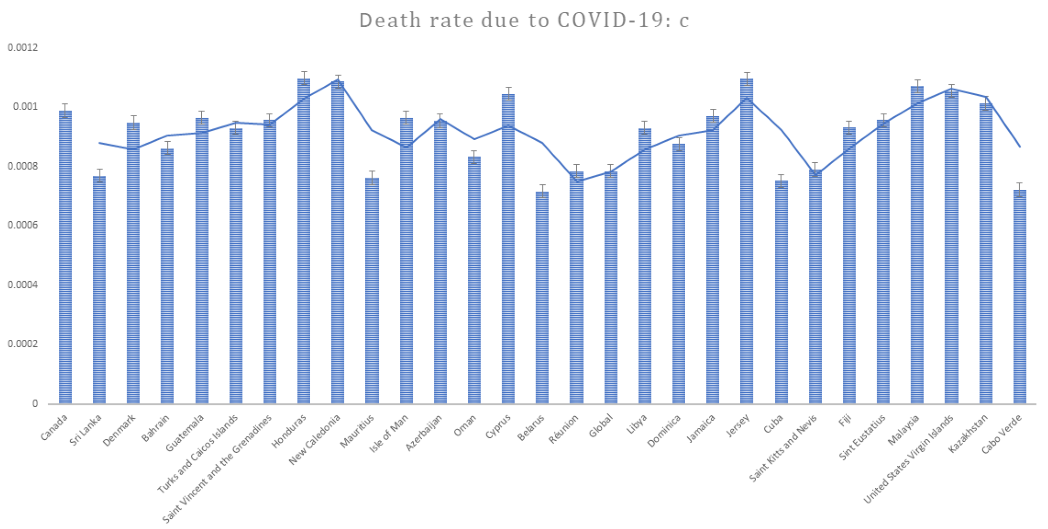
COVID-19 mortality rate: c

Based on data from the official website of The World Health Organization (https://www.who.int/, accessed on 14 March 2022), we can obtain the COVID-19 mortality rates of different countries. In order to ensure that the data can reflect the average, we take representative data and eliminate outliers. Finally, we screen the death rates due to disease for 29 countries. According to the data, we make a bar chart, which is presented in Figure 2.

From Figure 2, it is easy to find that the COVID-19 mortality rates of these countries are mostly in the range of 0.0008 to 0.001, so we choose the mean value of 0.0009 as the value of c.

(2) 

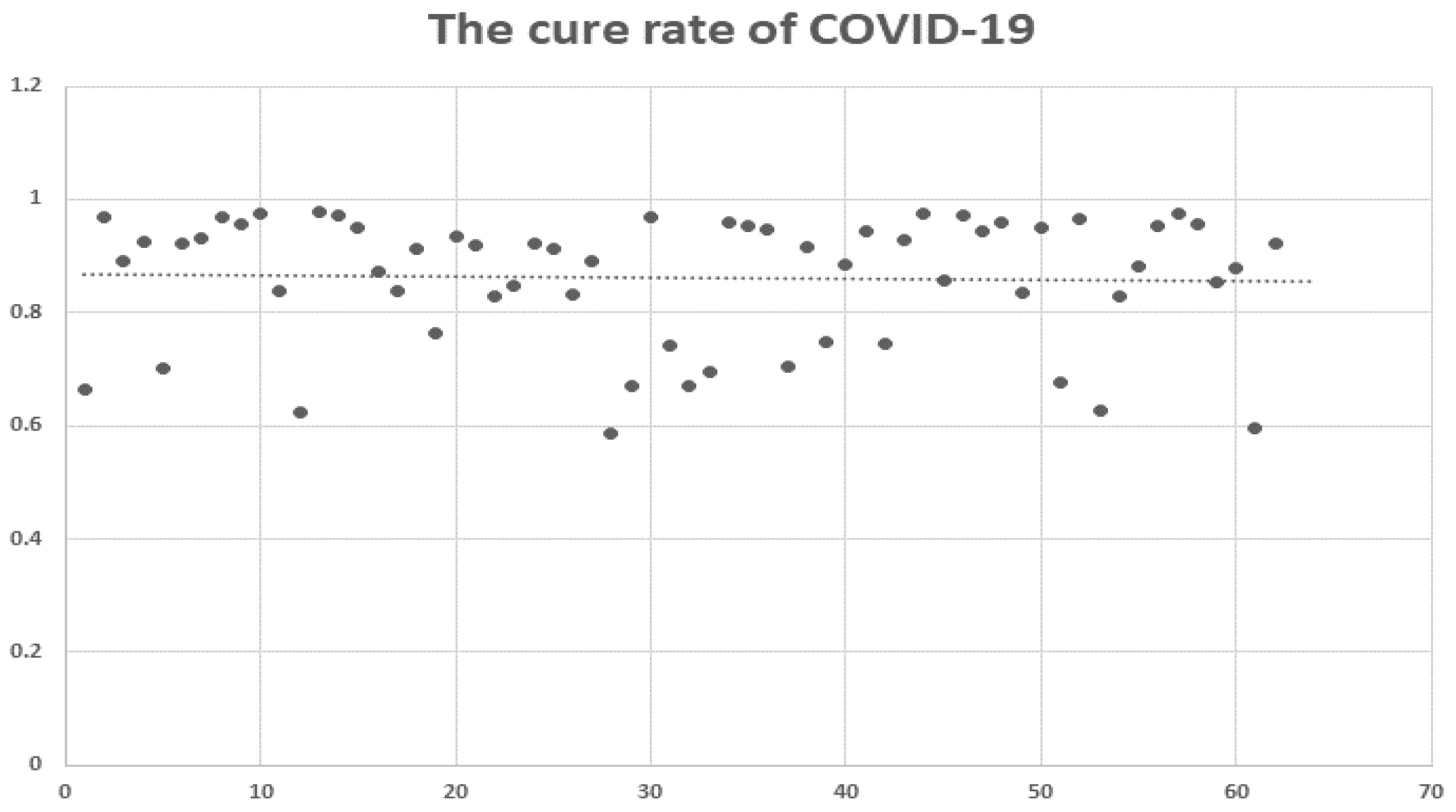
Cure rate: $\mu$

We obtained the cure rates of COVID-19 in different countries from the website of the WHO. By eliminating the missing values and outliers, we obtain the cure rates of 62 countries (such as the USA, Japan, Germany, Austria, Italy, Canada, South Africa, France and so on) and plot the scatter diagram in Figure 3.

As for cure rates $\mu$, we can clearly see that it is almost at the same level through the dotted line in Figure 3, so we figure out the average rate of 62 countries: 0.861 as the value of $\mu$.

(3) 

Infection rate: $\alpha$, $\beta$

Infection rates can vary from country to country because of the spread of the disease and the level of government concern. In addition, while antibodies are produced in vaccinated people, an immune barrier is not yet fully formed. So they also have some rate of transmission, but obviously, the people who get the booster vaccine have a lower rate of infection than the people who just get the basic vaccine. We consult the relevant data from the Centers for Disease Control and Prevention (https://www.cdc.gov/coronavirus/2019-ncov/index.html, accessed on 14 March 2022) and determine the values or range of $\alpha$ and $\beta$ in light of the actual situation. Then, we choose $\alpha =0.007$ and $\beta =0.0002$.

(4) 

Re-vaccination rate: ${\sigma }_1$, ${\sigma }_2$

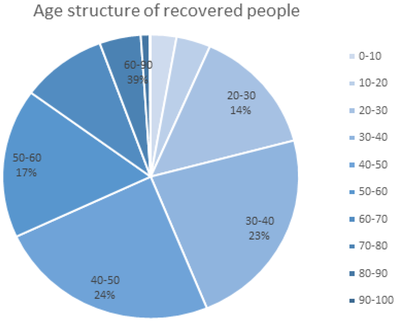
As we mentioned in the modeling, the level of antibody production after vaccination depends on the individual [22]. For people such as the elderly or those with underlying diseases who have recovered, the antibodies produced by the vaccine are almost completely disabled, and they need a basic injection to regain active antibodies at a conversion rate of ${\sigma }_1$ from R to S. In addition, some people still have some antibody activity in their bodies, and they only need to inject enhancers to increase their resistance to SARS-CoV-2 at a conversion rate of ${\sigma }_2$ from R to V. We think the difference is related to the age structure of the infected person (see Figure 4).

We find that recovered people between 20 and 50 years old account for 61% of the total, and we assume that this group has better physical fitness than other age groups. So we consider $\frac{{\sigma }_2}{{\sigma }_1}=1.6$, and choose ${\sigma }_1=0.2,\sigma =0.32$.

(5) 

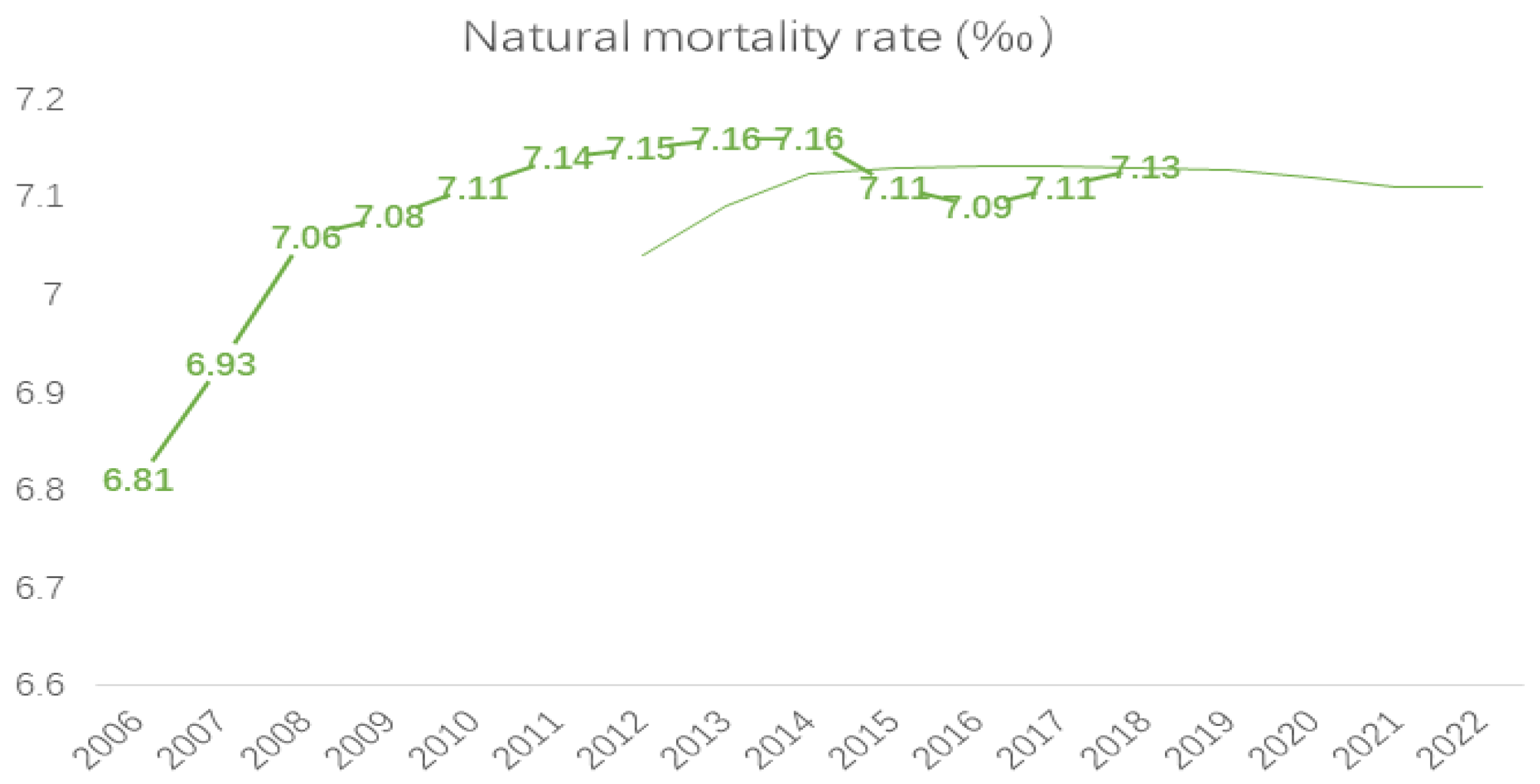
Natural mortality rate: d

In order to find the value of natural mortality rate d, we select population data from the National Bureau of Statistics (http://www.stats.gov.cn/enGliSH/, accessed on 14 March 2022) from 2006 to 2019, and we forecast a natural mortality rate $d=0.00707$ in 2022 based on trends (see Figure 5).

(6) 

Basic vaccination rate: $\Lambda$

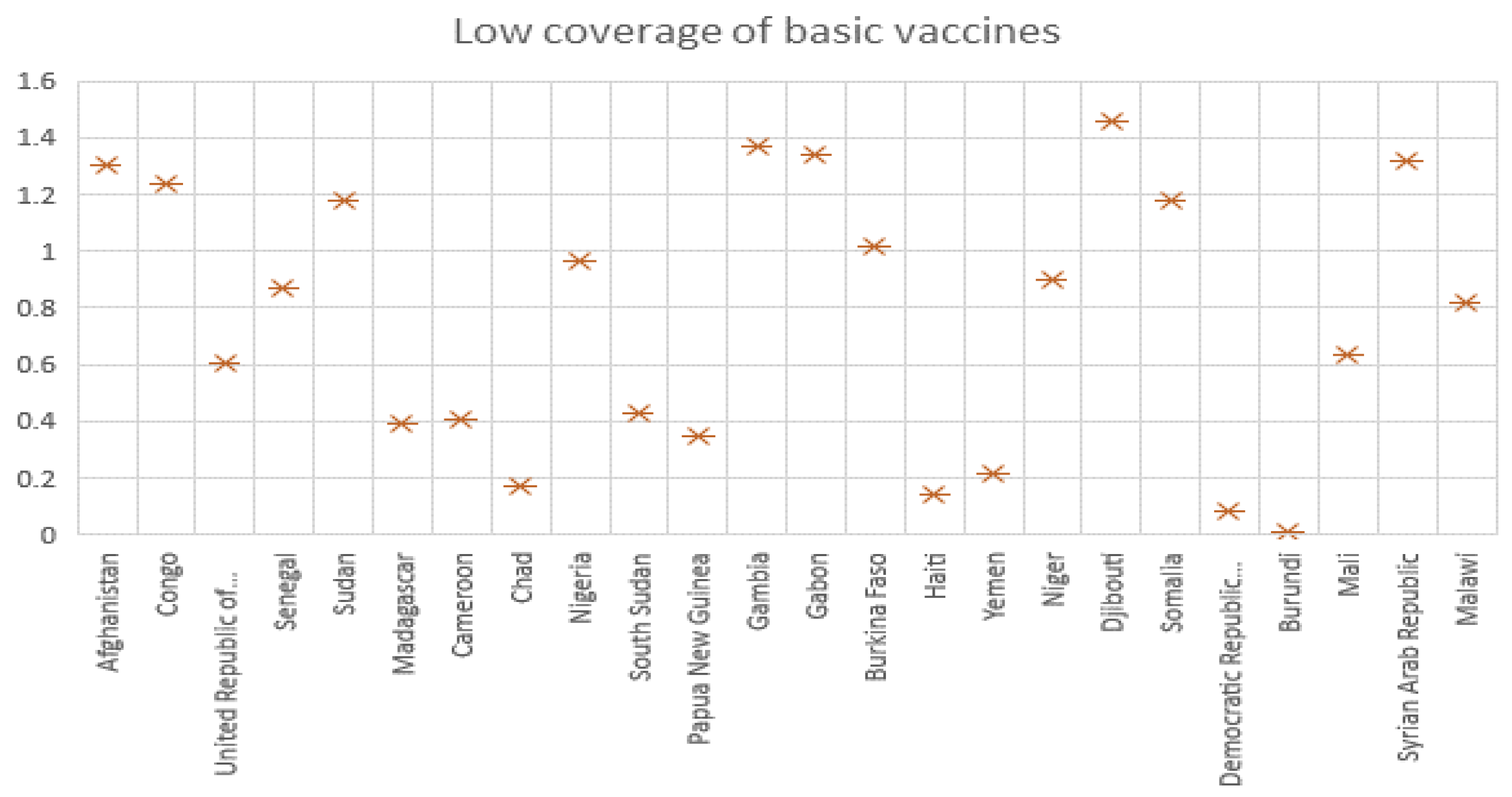
Due to limited vaccine resources in some countries or insufficient attention to the epidemic, vaccination rates vary significantly among countries. We classify countries in terms of high and low vaccination rates and discuss the impact of booster vaccination on epidemic control in both groups.

As we can see in Figure 6 and Figure 7, we classify the data provided by the WHO and select reasonable data to draw scatter plots. For countries with low vaccination rates, we find vaccination rates are around 0.8, so we select $\Lambda =0.8$ for the first set of parameters. For countries with high vaccination rates, in which people recognize the effectiveness of vaccines for epidemic control, vaccination rates reach 10, so we select $\Lambda =10$.

(7) 

Booster vaccination rate: ${\gamma }_1$

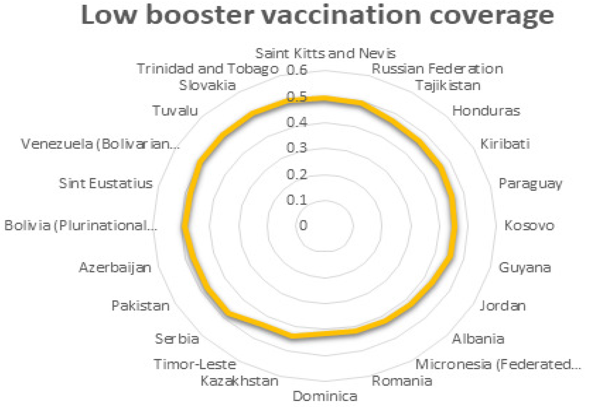
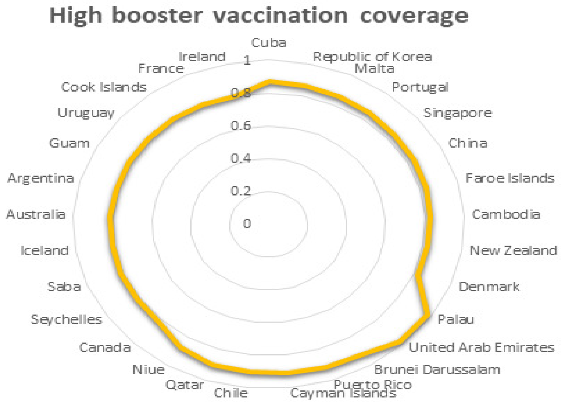
For booster vaccination, although the vaccination process is still going on and the rate of booster vaccination is still a variable, we can still analyze it based on the available data from the WHO because the level of national interest in vaccines does not change very much (see Figure 8 and Figure 9).

It is clear that the low booster vaccination rate is between 0.4 and 0.5, so we choose ${\gamma }_1=0.45$ as the booster vaccination rate for countries with low vaccination rates. In Figure 9, an average of 0.864 is selected as the booster vaccination rate for countries with high vaccination rates.

(8) 

The failure rate of booster vaccination: ${\gamma }_2$

As for ${\gamma }_2$, since the booster vaccine has just been developed, there is no exact failure rate and expiry time. Therefore, we refer to other vaccine-related data from the official website and select ${\gamma }_2=0.25$ as the failure rate of vaccines in countries with high vaccination rates and ${\gamma }_2=0.5$ as the failure rate of vaccines in countries with low vaccination rates, according to some experts’ prediction of the effectiveness of COVID-19 booster vaccines. To study the impact of a lower vaccine failure rate on epidemic control, we select ${\gamma }_2=0.15$ in the third group of parameters. This is consistent with the fact that the higher the failure rate, the less willing people are to be vaccinated.

Based on the above consideration, we take the following two groups of parameters (our parameters are all dimensionless):

(I):

$\Lambda =0.8,d=0.00707,\mu =0.861,c=0.0009,\alpha =0.007,\beta =0.0002,{\gamma }_1=0.45,{\gamma }_2=0.5,{\sigma }_1=0.2,{\sigma }_2=0.32;$

(II):

$\Lambda =10,d=0.00707,\mu =0.861,c=0.0009,\alpha =0.007,\beta =0.0002,{\gamma }_1=0.864,{\gamma }_2=0.25,{\sigma }_1=0.2,{\sigma }_2=0.32;$

(III):

$\Lambda =10,d=0.00707,\mu =0.861,c=0.0009,\alpha =0.007,\beta =0.0002,{\gamma }_1=0.864,{\gamma }_2=0.15,{\sigma }_1=0.246,{\sigma }_2=0.22.$

Parameter (I) simulates countries with low vaccination rates and low vaccine effectiveness, probably due to limited national resources and low level of development; Parameter (II) simulates countries with high vaccination rates and average vaccine effectiveness, which is consistent with the current reality of most countries; In order to study methods that can better control the epidemic, we select a third group of parameters (III), which reduced the failure rate compared with the second group of parameters.

5.2. Simulations and Verification

For the group of parameters (I):

$$\Lambda =0.8,d=0.00707,\mu =0.861,c=0.0009,\alpha =0.007,$$

$$\beta =0.0002,{\gamma }_1=0.45,{\gamma }_2=0.5,{\sigma }_1=0.2,{\sigma }_2=0.32.$$

This represents countries with low vaccination rates. We calculate the disease-free equilibrium $E_1=[59.95,53.20,0,0]$. Under this group of parameters, $R_0<1$, so equilibria $E_{2_l}$ do not exist, and $E_1=[59.95,53.20,0,0]$ is locally asymptotically stable when ${\tau }_1={\tau }_2=0$ according to Theorem 1 and Theorem 2. When ${\tau }_1>0,{\tau }_2=0$, $h\left(z\right)$ only has one positive root, and ${\omega }_{11}=0.0724$, $\sin \left({\omega }_{11}{\tau }_{21}^{\left(0\right)}\right)=0.1448$, $\cos \left({\omega }_{11}{\tau }_{21}^{\left(0\right)}\right)=-0.9141$, ${\tau }_{21}^{\left(0\right)}=37.62$. We choose ${\tau }_2={\tau }_{2*}=24$ and substitute it into Equations (12) and (13); we get ${\tilde{\omega }}_{11}=0.3814$, $\sin \left({\tilde{\omega }}_{11}{\tau }_{11}^{\left(0\right)}\right)=0.5218$, $\cos \left({\tilde{\omega }}_{11}{\tau }_{11}^{\left(0\right)}\right)=0.8530$, ${\tau }_{11}^{\left(0\right)}=1.44$. If (H5) holds, the equilibrium $E_1$ is locally asymptotically stable when ${\tau }_1\in \left[\left.0,{\tau }_{1*}\right)\right.$.

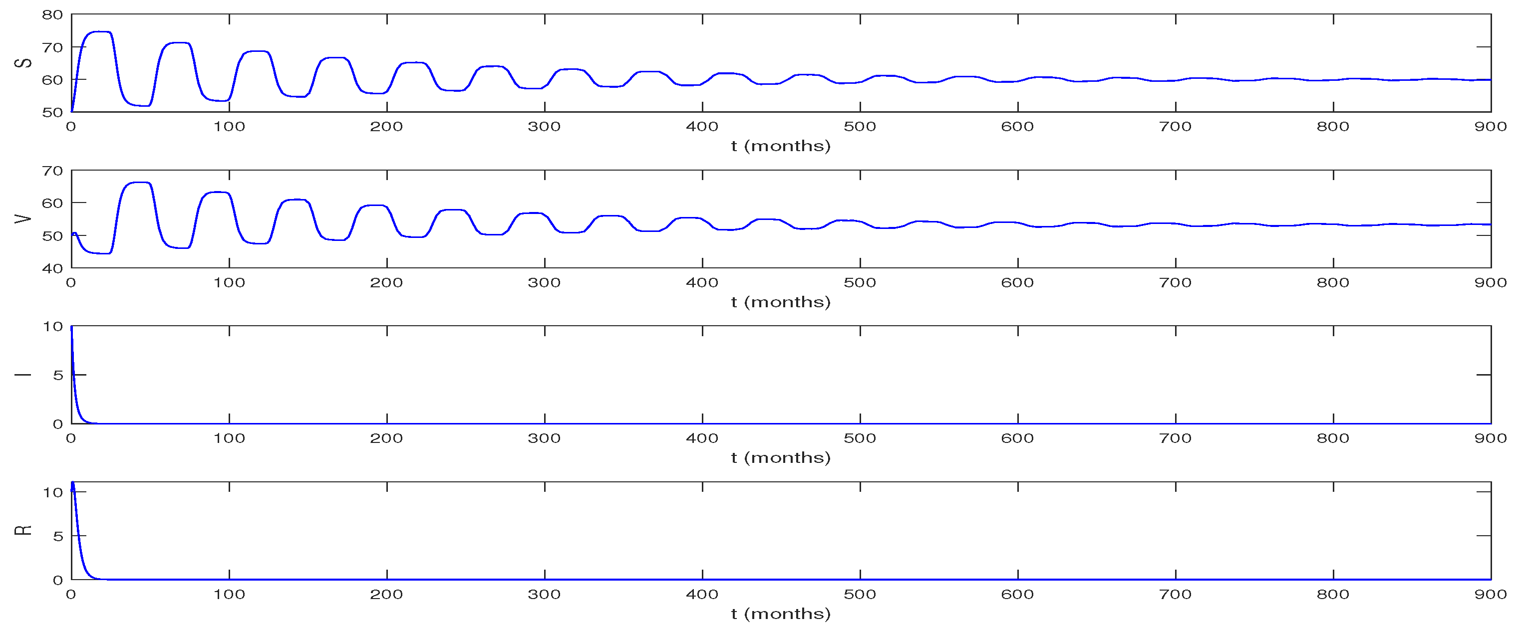
When ${\tau }_{2*}=24\in (0,{\tau }_{21}^{\left(0\right)})=(0,37.62)$, ${\tau }_{1*}=1\in (0,{\tau }_{11}^{\left(0\right)})=(0,1.44)$, the equilibrium $E_1$ is locally asymptotically stable according to Theorem 1; ${\tau }_{2*}=24$ means the vaccine will fail 24 months after injection and ${\tau }_{1*}=1$ means that people begin to inject booster vaccinations after 1 month to cope with the decrease of vaccine effectiveness. We choose initial values [50, 50, 10, 10] and picture the number of people in different cabins changing over time in Figure 10.

The figure above shows that when the vaccine is available for two years, people who get a booster vaccine within a month of getting the basic vaccine can get rid of all infections within 20 months. In other words, herd immunity is achieved before the vaccine wears off. S and V will stabilize after 400 months, and the epidemic will completely disappear.

Remark 1: 

Our simulations show that for low-coverage countries, when the vaccine is valid for two years, people need to receive the booster vaccine promptly within one and a half months of receiving the basic vaccine. After 1.5 months, an outbreak will occur. Further, the faster people are vaccinated, the more effectively the epidemic is contained. However, it became clear that getting a booster vaccine after a month would not meet the requirements of the vaccine for the human body. Most of these countries are currently experiencing outbreaks. This is consistent with our simulation results.

For the group of parameters (II):

$$\Lambda =10,d=0.00707,\mu =0.861,c=0.0009,\alpha =0.007,$$

$$\beta =0.0002,{\gamma }_1=0.864,{\gamma }_2=0.25,{\sigma }_1=0.2,{\sigma }_2=0.32.$$

This represents the situation for countries with high vaccination rates and average vaccine effectiveness. We find $R_0>1$, so equilibrium $E_{2_1}$ make sense and is [104.47, 688.37, 255.14, 367.79]. Equilibrium $E_1$ is unstable. Substituting this group of parameters into Equation (14), (H6) is satisfied, so equilibrium $E_{2_1}$ is locally asymptotically stable when ${\tau }_1={\tau }_2=0$ according to Theorem 2. When ${\tau }_1=0,{\tau }_2>0$, $h\left(z\right)$ only has one positive root, and ${\omega }_{21}=0.0805$, ${\tau }_{22,1}^{\left(0\right)}=28.50$. Selecting ${\tau }_{2*}=25$, we obtain ${\tilde{\omega }}_{21}=0.2157$, $\sin \left({\tilde{\omega }}_{21}{\tau }_{12,1}^{\left(0\right)}\right)=0.8118$, $\cos \left({\tilde{\omega }}_{21}{\tau }_{12,1}^{\left(0\right)}\right)=-0.5840$, ${\tau }_{12,1}^{\left(0\right)}=10.17$. Substituting the parameters (II) into Equations (A9) and (A14), we have $\mathrm{Re}\left(M_k\right)>0,\mathrm{Re}\left(H_k\right)<0$. According to Theorem 3, we can deduce ${\tau }_{\epsilon }>0$, $\mathrm{Re}\left(M_k\right){\tau }_{\epsilon }>0$; the periodic solution is stable. This means that the epidemic will fluctuate greatly over time, and people’s means of controlling the epidemic have no obvious effect on controlling the epidemic. However, there will not be a sudden increase in the number of infected people at a certain moment, and the epidemic situation will not be uncontrollable.

Considering the vaccine developed at present is not an instantaneous failure, and vaccines cannot be administered in a short time, ${\tau }_1={\tau }_2=0$ is impossible.

According to existing medical research, we believe that the validity period of the vaccine is 23–32 months, so we choose ${\tau }_{2*}=25$ as the validity period of a booster vaccine. Our purpose is to study the impact of different booster vaccine inoculation times on the epidemic situation. Through our simulation under this set of parameters, we find two important time nodes—6 months and 10 months—to get booster vaccination after basic vaccination. Vaccination after 10 months will lead to an outbreak, which is consistent with our theoretical analysis. Vaccination within six months makes a difference in the epidemic compared to the situation in which people get vaccinated after 6 months.

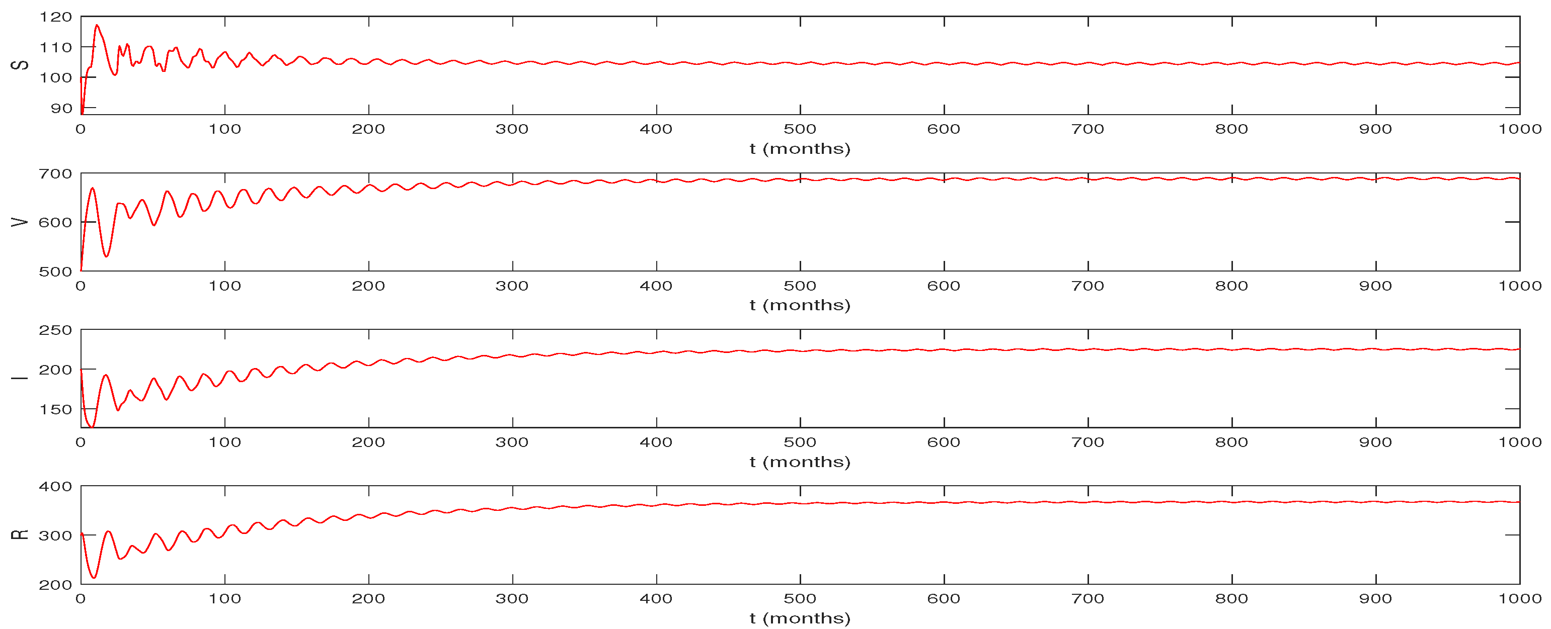
When ${\tau }_{2*}=25,{\tau }_{1*}=7$ that means the vaccine will expire after 25 months and booster vaccination will be carried out after 7 months. We still choose [100, 500, 200, 300] as the initial values; the epidemic situation is shown in Figure 11.

While the vaccine is still valid for 25 months, people getting booster shots within 7 months will have an overall increase in infections for 500 months, meaning that the number of infections will be high for a long time. This situation can only keep the epidemic under control but does not reduce the number of infected people.

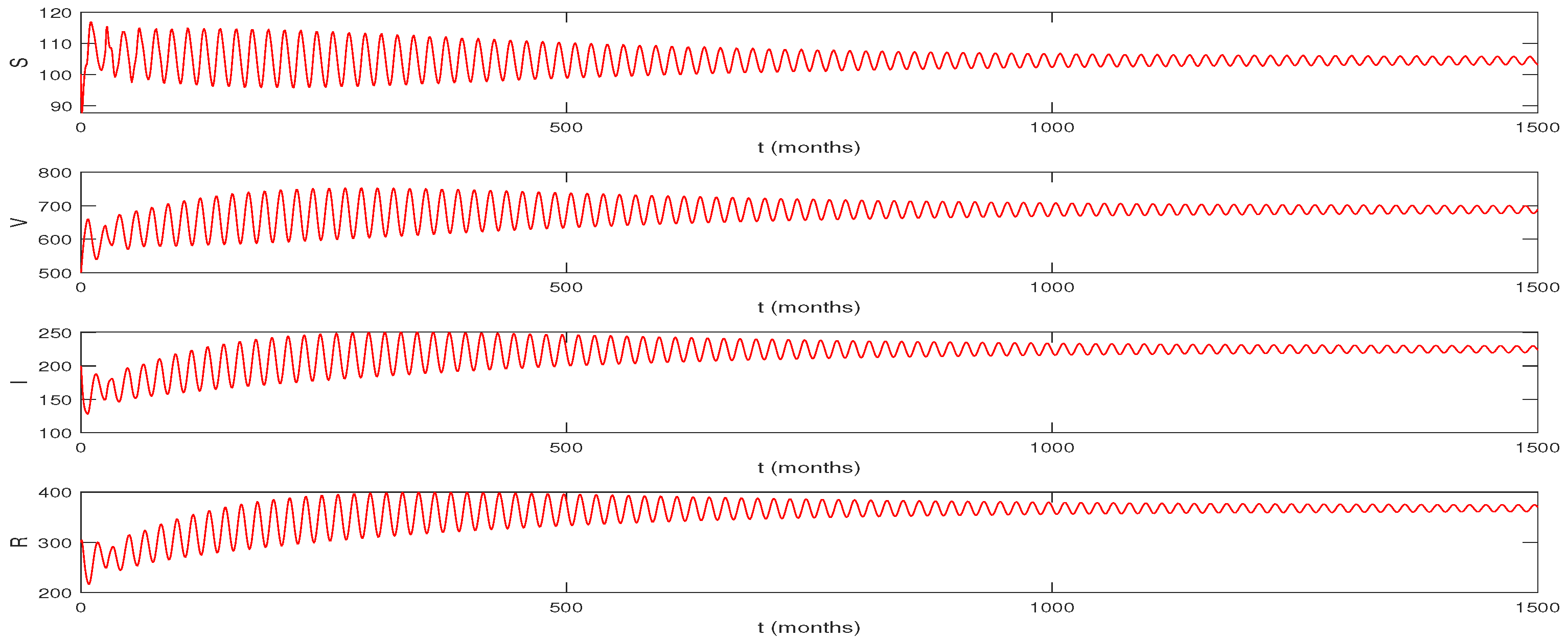
When ${\tau }_{2*}=25\in (0,{\tau }_{22,1}^{\left(0\right)})=(0,28.5),{\tau }_{1*}=6\in (0,{\tau }_{12,1}^{\left(0\right)})=(0,10.17)$ that means the vaccine expire after 25 months, and we inject the booster vaccine after 6 months; we choose [100, 500, 200, 300] as the initial values (see Figure 12).

We can see that the epidemic has fluctuated over 500 months. This is consistent with our reality. Currently, we are required to get a booster shot six months after the basic vaccine. Even then, the epidemic does not disappear completely. There are periodic fastigiums in the number of infections. However, by vaccinating we can prevent the number of infections from increasing or staying high and stabilize the epidemic over many years. That is, the booster vaccination has a positive effect on the development of the epidemic, and the trend will be better with the booster vaccination in time.

Remark 2: 

This means that under this set of parameters, people will inevitably live with the virus for a long time, and a booster vaccination at the right time will only have a temporary effect on reducing the number of infections.

For the group of parameters (III):

$$\Lambda =10,d=0.00707,\mu =0.861,0.0009,\alpha =0.007,$$

$$\beta =0.0002,{\gamma }_1=0.864,{\gamma }_2=0.15,{\sigma }_1=0.246,{\sigma }_2=0.22.$$

This set of parameters represents the ideal situation in which the outbreak can be well contained. We find $R_0>1$, so equilibrium $E_{2_1}$ makes sense and is [100.92, 812.57, 169.97, 309.34]. Equilibrium $E_1$ is unstable. Substituting this group of parameters into Equation (14), (H6) is satisfied, so equilibrium $E_{2_1}$ is locally asymptotically stable when ${\tau }_1={\tau }_2=0$ according to Theorem 2. When ${\tau }_1=0,{\tau }_2>0$, $h\left(z\right)$ only has one positive root, and ${\omega }_{21}=0.0576$, ${\tau }_{22,1}^{\left(0\right)}=38.78$. Selecting ${\tau }_{2*}=32$, we obtain ${\tilde{\omega }}_{21}=0.1152$, $\sin \left({\tilde{\omega }}_{21}{\tau }_{12,1}^{\left(0\right)}\right)=0.7078$, $\cos \left({\tilde{\omega }}_{21}{\tau }_{12,1}^{\left(0\right)}\right)=-0.7064$, ${\tau }_{12,1}^{\left(0\right)}=20.44$. Substituting the parameters (II) into Equations (A9) and (A14), we have $\mathrm{Re}\left(M_k\right)>0,\mathrm{Re}\left(H_k\right)<0$. According to Theorem 3, we can deduce ${\tau }_{\epsilon }>0$, $\mathrm{Re}\left(M_k\right){\tau }_{\epsilon }>0$, which means under this set of parameters, if the equilibrium $E_{2_1}$ is unstable, a stable Hopf bifurcation periodic solution will appear. This means that although there will not be a large number of people infected with the novel coronavirus and the number of cases will surge, people’s methods are still ineffective, and people need to find better ways to control the epidemic.

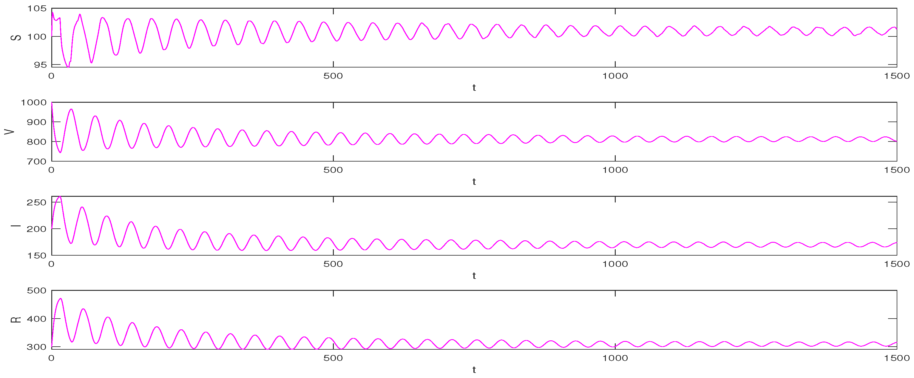
When ${\tau }_{2*}=32\in (0,{\tau }_{22,1}^{\left(0\right)})=(0,38.78),{\tau }_{1*}=6\in (0,{\tau }_{12,1}^{\left(0\right)})=(0,20.44)$ that means the vaccine expires after 32 months and people inject the booster vaccine after 6 months, we choose [100, 1000, 200, 300] as the initial values (see Figure 13).

Figure 13 shows a declining trend in the number of infections under the third set of parameters, which stabilizes and approaches almost zero after two decades. This suggests that when the validity of the vaccine is increased to 32 months and the vaccine failure rate is reduced to 0.15, people who receive the booster vaccine 6 months after the basic vaccine can control the outbreak more effectively without long-term coexistence with the virus. In other words, if the vaccine is effective enough, we can expect to be free of COVID-19 by 2042 or earlier. However, this is a relatively ideal situation because many factors in reality can cause the values of parameters in the model to change at any time, and our simulation is based on only a set of constant parameters.

To make the simulation results closer to reality, we can change the value of parameters in real-time according to the actual situation of the epidemic development and use our model to predict the development of the epidemic under different factors such as infection rate, cure rate and vaccine effectiveness. We can provide ideas for the country to control the epidemic by analyzing the simulation results.

When ${\tau }_{2*}=32,{\tau }_{1*}=14.5$ that means the vaccine expires after 32 months, but people inject the booster vaccine after 14.5 months; we choose [100, 1000, 200, 300] as the initial values (see Figure 14).

Remark 3: 

Comparing Figure 13 with Figure 14, it can be found that when the booster vaccination time is 14.5 months, although the system fluctuation trend becomes smaller and the number of infected people also decreases, it takes longer for the system to stabilize than when the booster vaccination time is 6 months. As shown in Figure 14, the system is not stable after 500 months, which has a bad impact on the country’s economy and development. Therefore, it is necessary to implement the booster vaccine as soon as the effectiveness of the vaccine is certain.

5.3. Analysis of Simulations

Based on the above simulations, we have the following conclusions:

(1) When the time of vaccine expiration is determined, the less time people have between a basic vaccine and a booster, the better the outbreak will be contained in both low and high coverage countries, and when the time of booster vaccination exceeds the critical value, System (1) will be unstable and the epidemic will be out of control. The critical time for the booster vaccination is 1.4 months for countries with low vaccination rates and 10.17 months for countries with high vaccination rates. It is clear that increasing vaccination rates have had a positive impact on epidemic control.

(2) We select the parameters (I) and (II) closest to the current epidemic situation, and the simulation results are consistent with the real situation. Due to limited vaccine resources or other reasons, some countries have low vaccination rates. For them, booster vaccination is not completed effectively and on time. As for the critical time of 1.44 months in our simulation results, it is impossible to complete in reality. We look at the epidemic status of most countries with low vaccination rates and found that most of them are in an uncontrolled state of the epidemic, which is consistent with our simulations. For countries with high vaccination rates, we found that the critical time for booster vaccination is 10.17 months, which can be achieved in reality. Given the physical demands of vaccination, most countries require people to receive the booster vaccine promptly 6 months after receiving the basic vaccine. In our simulations, 6 months is also considered to be the most suitable optimal time for booster vaccination. In this case, there will be some fluctuations in the current epidemic, but the number of infections will not be at a high level all the time, and people will be able to control the epidemic within a certain range and eventually stabilize it. When the inoculation time is 7 months, although the epidemic does not fluctuate greatly in the near stage and eventually tends to stabilize, the number of infected people will remain at a high level. This means that under the second set of parameters, the effectiveness of the vaccine will not be enough to eliminate the epidemic, and even if people are actively vaccinated and have high vaccination rates, they will inevitably live with COVID-19 for a long time.

(3) Due to the short development time of the vaccine, its effectiveness is still unclear. In our numerical simulations, different parameters are used to study the impact of vaccine effectiveness on the epidemic. We choose parameters (III) to simulate a better epidemic scenario. Compared with the groups of parameters (I) and (II), the third group has a higher vaccination rate and lower vaccine failure rate, the basal shot is less likely to fail, and the proportion of recovered patients who retain antibodies from the basal shot increased. Through our simulation, we found that under the third set of parameters, when the validity of the vaccine is 32 months and the booster vaccination time is controlled within 20 months, the number of infections decreased and eventually approached zero, the system stabilized, and the epidemic almost disappeared. Changing the timing of the booster vaccine, we found that when the booster vaccine is given at 6 months, the epidemic could be virtually eliminated by 2042. Even though the parameters can change over time in the real world, and this is an ideal situation for us to simulate with a constant set of parameters, we can still conclude that the longer the interval between actual vaccinations, the longer it takes for the epidemic to stabilize. Therefore, considering the economic level of the country and the requirements of the vaccine for the human body, we believe that under the third group of parameters we selected, timely vaccination after 6 months is the ideal epidemic control means.

Compared with the second group of parameters (II), the failure rate of the third group (III) of enhanced vaccines is reduced, the validity period is longer, and the epidemic can be effectively controlled, or even almost disappear. Under the second set of parameters (II), the vaccine is not effective enough, and the epidemic continues. This shows the importance of vaccine effectiveness in controlling outbreaks. In order to better control the epidemic, we need to work to develop a more effective vaccine.

(4) In our simulations above, we select parameters consistent with the current epidemic situation in 2022 and obtain simulation results consistent with the real situation. In fact, our simulations can change with reality, which means that our models are very broad. For example, if a country wants to study epidemic prevention and control strategies for itself, we can bring in the country’s data, take into account the comprehensive strength of the country and the requirements of economic development, analyze the data and select reasonable parameters for simulation to obtain the best time for strengthening vaccination and provide targeted strategies for epidemic control. Our model can also simulate the situation as the virus mutates by changing the infection rate $\alpha$ and $\beta$. Global vaccination is still ongoing, so vaccination rates are constantly changing, and we can change the vaccination rates in the parameters to change our conclusions in real-time. Once the parameters are determined, we can calculate the corresponding critical booster timing and make recommendations that are appropriate to the current epidemic situation.

5.4. Recommendations for Countries

(i)

For countries with low vaccination rates:

Based on our simulations, it is clear that good control of the epidemic requires people to get the booster vaccine within 1.5 months of getting the basic vaccine. However, a 1.5-month interval between basic and booster vaccination is not feasible in real life given the requirements of the vaccine for people’s health conditions. That means it is very difficult to control COVID-19 in these countries. Therefore, we call on countries with low vaccination rates to increase their vaccination rates as soon as possible so that people pay enough attention to COVID-19;otherwise, it will be difficult to control the epidemic.

(ii)

For countries with high vaccination rates:

(1) It is clear that timely booster vaccination has a positive impact on controlling the outbreak. Controlling booster vaccination time within a critical period (10.2 months) can make sure the epidemic is under control. Considering the requirements of booster vaccination on the body, we believe that 6 months is the most appropriate time for booster vaccination.

(2) In countries that are already able to get the majority of people who get the basic vaccine on time to get the booster vaccine 6 months later, we can see that there is an upper bound in the number of infections in those countries, which means that the epidemic is contained, and the number of infections does not peak all the time. However, the epidemic is not completely under control. In these countries, the epidemic is cyclical at this stage, with the number of cases going up and down. However, when we improve the effectiveness of the vaccine, which means the duration of the vaccine is longer and the failure rate of the vaccine is lower, the epidemic will be better controlled. The number of cases tends to decrease and almost stabilize after 20 years. So we suggest that research into an effective vaccine should continue, both to increase its longevity and to reduce the vaccine failure rate.

(3) Considering that the virus is still mutating, we suggest that countries make timely policy changes based on the real-time situation of the epidemic.

6. Conclusions

In this paper, we have established an SVIR model on booster vaccination with two time delays to study the most suitable time for booster vaccination. We have studied the impact of the timing of booster vaccination and the expiration of booster vaccine on outbreaks. We studied the stability of the equilibria of System (1) and determine the stability and direction of the periodic bifurcation solution using the multi-time scale method and obtain the standard form of Hopf bifurcation. Then we have carried out some numerical simulations to verify the analytic results and give some reasonable suggestions to control the epidemic.

We have found that high vaccination rates are necessary for the current epidemic situation and that current vaccines are not effective as a specific method of controlling the epidemic. As well as improving vaccination rates, there are other measures that need to be taken, such as reducing social interaction. Further, we have specific recommendations for different countries as well.

References

- Nathan, D.G.; Emma, B.H.; Joseph, R.F.; Alexandra, L.P. MugeCevik Public health actions to control new SARS-CoV-2 variants. Cell 2021, 184, 1127–1132. [Google Scholar]
- Pei, Y.Z.; Li, S.P.; Li, C.G.; Chen, S.Z. The effect of constant and pulse vaccination on an SIR epidemic model with infectious period. Appl. Math. Model. 2011, 35, 3866–3878. [Google Scholar]
- Cao, B.Q.; Shan, M.J.; Zhang, Q.M.; Wang, W.M. A stochastic SIS epidemic model with vaccination. Physica A 2017, 486, 127–143. [Google Scholar] [CrossRef]
- De la Sen, M.; Alonso-Quesada, S. Vaccination strategies based on feedback control techniques for a general SEIR-epidemic model. Appl. Math. Comput. 2011, 218, 3888–3904. [Google Scholar] [CrossRef]
- Khyar, O.; Allali, K. Optimal vaccination strategy for an SEIR model of infectious diseases with Logistic growth. Math. Biosci. Eng. 2017, 15, 485–505. [Google Scholar]
- Scherer, A.; McLean, A. Mathematical models of vaccination. Brit. Med. Bull. 2002, 62, 187–199. [Google Scholar] [CrossRef] [Green Version]
- Bjornstad, O.N.; Shea, K.; Krzywinski, M.; Altman, N. The SEIRS model for infectious disease dynamics. Nat. Methods 2020, 17, 557–558. [Google Scholar] [CrossRef]
- Yang, B.; Yu, Z.H.; Cai, Y.L. The impact of vaccination on the spread of COVID-19: Studying by a mathematical model. Nonlinear Dyn. 2022, 590, 126717. [Google Scholar] [CrossRef]
- Duan, X.C.; Yuan, S.l.; Li, X.Z. Global stability of an SVIR model with age of vaccination. Appl. Math Comput. 2014, 226, 528–540. [Google Scholar] [CrossRef]
- Anna, W. Booster Vaccination to Reduce SARS-CoV-2 Transmission and Infection. JAMA-J. Am. Med. Assoc. 2012, 327, 327–328. [Google Scholar]
- Salvagno, G.L.; Henry, B.M.; Pighi, L.D.N.; Simone, D.N.; Gianluca, G.; Giuseppe, L. The pronounced decline of anti-SARS-CoV-2 spike trimeric IgG and RBD IgG in baseline seronegative individuals six months after BNT162b2 vaccination is consistent with the need for vaccine boosters. Clin. Chem. Lab. Med. 2022, 60, E29–E31. [Google Scholar] [CrossRef] [PubMed]
- Cooke, K.L. Stability analysis for a vector disease model. J. Math. Biol. 1996, 35, 240–260. [Google Scholar] [CrossRef] [PubMed]
- Zhai, S.D.; Luo, G.Q.; Huang, T.; Wang, X.; Tao, J.L.; Zhou, P. Vaccination control of an epidemic model with time delay and its application to COVID-19. Nonlinear Dyn. 2021, 106, 1279–1292. [Google Scholar] [CrossRef] [PubMed]
- Rong, X.M.; Yang, L.; Chu, H.D.; Fan, M. Effect of delay in diagnosis on transmission of COVID-19. Math. Biosci. Eng. 2020, 17, 2725–2740. [Google Scholar] [CrossRef]
- Song, X.Y.; Jiang, Y.; Wei, H.M. Analysis of a saturation incidence SVEIRS epidemic model with pulse and two time delays. Appl. Math. Comput. 2009, 214, 381–390. [Google Scholar] [CrossRef]
- Jiang, Y.; Mei, L.Q.; Song, X.Y. Global analysis of a delayed epidemic dynamical system with pulse vaccination and nonlinear incidence rate. Appl. Math. Model. 2011, 35, 4865–4876. [Google Scholar] [CrossRef]
- Gao, S.J.; Teng, Z.D.; Xie, D.H. The effects of pulse vaccination on SEIR model with two time delays. Appl. Math. Comput. 2008, 201, 282–292. [Google Scholar] [CrossRef]
- Zhang, Z.Z.; Kundu, S.; Tripathi, J.P.; Bugalia, S. Stability and Hopf bifurcation analysis of an SVEIR epidemic model with vaccination and multiple time delays. Chaos Soliton Fract. 2020, 131, 109483. [Google Scholar] [CrossRef]
- Chen, X.Y.; Cao, J.D.; Park, J.H.; Qiu, J.L. Stability analysis and estimation of domain of attraction for the endemic equilibrium of an SEIQ epidemic model. Nonlinear Dynam. 2018, 87, 975–985. [Google Scholar] [CrossRef]
- Li, J.H.; Teng, Z.D.; Wang, G.Q.; Zhang, L.; Hu, C. Stability and bifurcation analysis of an SIR epidemic model with logistic growth and saturated treatment. Chaos Soliton Fract. 2017, 99, 63–71. [Google Scholar] [CrossRef]
- Goel, K.; Kumar, A. Nilam Stability analysis of a logistic growth epidemic model with two explicit time-delays, the nonlinear incidence and treatment rates. J. Appl. Math. Comput. 2021, 389–402. [Google Scholar]
- Hye, K.L.; Ludwig, K.; Ludwig, K.S.; Sebastian, K.; Birgit, P. Robust immune response to the BNT162b mRNA vaccine in an elderly population vaccinated 15 months after recovery from COVID-19. MedRxiv Preprint 2021, 5. [Google Scholar] [CrossRef]
Figure 1.
SVIR Model diagram.
Figure 2.
COVID-19 mortality rates of 29 countries.
Figure 3.
Cure rates of COVID-19 of 62 countries.
Figure 4.
Age structure of recovered people.
Figure 5.
Natural mortality rate.
Figure 6.
The basic vaccination rates of 24 countries with low vaccination rates.
Figure 7.
The basic vaccination rates of 23 countries with high vaccination rates.
Figure 8.
The booster vaccination rates of 24 countries with low vaccination rates.
Figure 9.
The booster vaccination rates of 29 countries with high vaccination rates.
Figure 10.
When , , equilibrium of System (1) is locally asymptotically stable.
Figure 11.
, , equilibrium of System (1) is locally asymptotically stable.
Figure 12.
Figure 13.
Figure 14.