Optimum Approximation for ς–Lie Homomorphisms and Jordan ς–Lie Homomorphisms in ς–Lie Algebras by Aggregation Control Functions

Abstract

In this work, by considering a class of matrix valued fuzzy controllers and using a $(\kappa ,\varsigma )$-Cauchy–Jensen additive functional equation ($(\kappa ,\varsigma )$-CJAFE), we apply the Radu–Mihet method (RMM), which is derived from an alternative fixed point theorem, and obtain the existence of a unique solution and the H–U–R stability (Hyers–Ulam–Rassias) for the homomorphisms and Jordan homomorphisms on Lie matrix valued fuzzy algebras with $\varsigma$ members ($\varsigma$-LMVFA). With regards to each theorem, we consider the aggregation function as a matrix value fuzzy control function and investigate the results obtained.

1. Introduction

Lie algebras are named after the Norwegian mathematician Sophus Lie (1842–1899). Most of what we know about the original formulation comes from Lie’s lecture notes in Leipzig, as collected by Scheffers. For $\varsigma \ge 0$, Lie algebras with $\varsigma$ members ($\varsigma$- LA), which was first introduced in 1985 by Filippov [1], are n-linear, antisymmetric, and satisfy a generalization of the Jacobi identity. The definition of $\varsigma$- LA for $\varsigma =3$ was first proposed by Nambu in 1973 [2]. On a field like $\mathbb{Q}$, a structure of $\varsigma$- LA with the finite dimension was developed of zero. Additionally, many researchers, to find the effect of $M2$-branes in the M-theory, which in this theory starts with the BLG (Bagger–Lambert–Gustavsson) model, have considered $\varsigma$-ary algebras in the Nambu mechanical in the field of physics [1,3,4,5].

The issue of the stability of functional equations was first raised by Ulam about the stability of group homomorphisms in 1940 [6]. Hyers in 1941, developed H–U type stability for functional equations by finding a homomorphism near an approximate homomorphism. To continue Hyers’ work and to develop the problem of stability, additive mappings and linear mappings were investigated by Aoki and Rassias. A generalization of the stability of linear maps was also done by Găvruţă [7,8,9]. The equation we are considering is defined as follows

$$\begin{array}{c}\hfill \sum _{\begin{array}{c}1\le {\mathit{a}}_1<\cdots <{\mathit{a}}_{\kappa }\le \varsigma \hfill \\ 1\le {\alpha }_{\iota }\le \varsigma \hfill \\ {\alpha }_{\iota }\ne {\mathit{a}}_{\mathit{b}},\forall \mathit{b}\in \{1,\dots ,\kappa \}\hfill \end{array}}\Theta \left(\frac{{\displaystyle \sum _{\mathit{b}=\mathit{a}}^{\kappa }}{\omega }_{{\mathit{a}}_{\mathit{b}}}}{\kappa }+\sum _{\iota =1}^{\varsigma -\kappa }{\omega }_{{\alpha }_{\iota }}\right)=\frac{(\varsigma -\kappa +1)\left(\begin{array}{c}\varsigma \\ \kappa \end{array}\right){\displaystyle \sum _{i=1}^{\varsigma }}\Theta \left({\omega }_{\mathit{a}}\right)}{\varsigma },\end{array}$$

(1)

which is a generalization of the CJAFE, for $\kappa ,\varsigma \in \mathbb{N}$, where $\varsigma \ge 2$ and $1\le \kappa \le \varsigma$. The solutions of Equation (1) are called $(\kappa ,\varsigma )$-CJA. Many researchers have worked on this equation. For example, Rassias and Kim investigated the generalized H–U stability for the above equation in quasi-$\beta$-normed spaces for $\kappa =2$ [10,11,12,13]. Our motivation in this work is to investigate the generalized H–U stability of the Lie homomorphisms and Jordan Lie homomorphisms related to the CJAFE function using the matrix value fuzzy controller aggregation function.

The order of our article is based on the following:

• We present the definition of $\varsigma$-LA and we introduce the matrix valued fuzzy normed space and the matrix valued fuzzy controllers.
• We apply Radu–Mihet method derived from the alternative fixed point theorem to study the H–U–R stability of homomorphisms and Jordan homomorphisms on $\varsigma$-LMVFBA.

2. Preliminaries

We begin this section with definitions of the functions and concepts we need to achieve the desired results. Since we investigate stability using the aggregation controller function, we introduce this function in this section.

Definition 1.

For $\varsigma \ge 3$, an ς-ary operation $\left[\right]:{\wedge }^{\varsigma }\mathcal{Z}\to \mathcal{Z}$ is an ς- ary Lie algebra or simpler ς-Lie algebra (ς-LA) if the following Jacobi identity holds

$$[[{\omega }_1,\dots ,{\omega }_{\varsigma }],{\omega }_{\varsigma +1},\dots ,{\omega }_{2\varsigma -1}]=\sum _{\mathit{a}=1}^{\varsigma }[{\omega }_1,\dots ,{\omega }_{\mathit{a}-1},[{\omega }_{\mathit{a}},{\omega }_{\varsigma +1}\dots ,{\omega }_{2\varsigma -1}],\dots ,{\omega }_{\varsigma }],$$

(2)

where $\mathcal{Z}$ is a vector space, ${\omega }_1,{\omega }_2,\dots ,{\omega }_{2\varsigma -1}\in \mathcal{Z}$ and operation $\left[\right]$ is multi-linear and antisymmetric.

Definition 2

([14]). The Mittag–Leffler function is given by the series

$$E_{\alpha }\left(\mathrm{g}\right)=\sum _{n=0}^{+\infty }\frac{{\mathrm{g}}^n}{\mathsf{\Gamma }(n\alpha +1)},$$

with $\alpha \in \mathbb{C}$, $Re\left(\alpha \right)>0$ and $\mathsf{\Gamma }\left(z\right)$ is a gamma function. The two parameters Mittag–Leffler function is given by the series

$$E_{\alpha ,\beta }\left(\mathrm{g}\right)=\sum _{n=0}^{+\infty }\frac{{\mathrm{g}}^n}{\mathsf{\Gamma }(n\alpha +\beta )},$$

with $\alpha ,\beta \in \mathbb{C}$, $Re\left(\alpha \right)>0$ and $Re\left(\beta \right)>0.$

Definition 3

([15,16]). According to a standard notation, the Fox $\mathcal{H}$ function is defined as

$${\mathcal{H}}_{p,q}^{m,n}\left(\mathfrak{g}\right)=\frac{1}{2\pi i}{\int }_{\mathcal{L}}{\mathcal{H}}_{p,q}^{m,n}\left(e\right){𝔤}^{e}de,$$

(3)

where $\mathcal{L}$ is a suitable path in the complex plane $\mathbb{C}$ to be disposed later. ${\mathfrak{g}}^e=exp\left\{\right(log\left|\mathfrak{g}\right|+iarg\mathfrak{g}\left)\right\}$ and

$${\mathcal{H}}_{p,q}^{m,n}\left(e\right)=\frac{\mathbb{V}\left(e\right)\mathbb{W}\left(e\right)}{\mathbb{X}\left(e\right)\mathbb{Y}\left(e\right)}$$

(4)

$$\begin{array}{cc}\hfill \mathbb{V}\left(e\right)=\prod _{j=1}^m\mathsf{\Gamma }({\mathit{s}}_j-{\psi }_{j}e),& \mathbb{W}\left(e\right)=\prod _{j=1}^n\mathsf{\Gamma }(1-{\mathit{r}}_j+{\varphi }_{j}e),\hfill \end{array}$$

(5)

$$\begin{array}{cc}\hfill \mathbb{X}\left(e\right)=\prod _{j=m+1}^q\mathsf{\Gamma }(1-{\mathit{s}}_j+{\psi }_{j}e),& \mathbb{Y}\left(e\right)=\prod _{j=n+1}^p\mathsf{\Gamma }({\mathit{r}}_j-{\varphi }_{j}e)\hfill \end{array}$$

(6)

with $0\le n\le p$, $1\le m\le q$, $\{{\mathit{r}}_j,{\mathit{s}}_j\}\in \mathbb{C}$, $\{{\varphi }_j,{\psi }_j\}\in {\mathbb{R}}^{+}$. An empty product, when it occurs, is taken to be one so $n=0$ if and only if $\mathbb{W}\left(e\right)=1$, $m=q$ if and only if $\mathbb{X}\left(e\right)=1$, $n=p$ if and only if $\mathbb{Y}\left(e\right)=1.$ Due to the occurrence of the factor ${\mathfrak{g}}^e$ in the integrand of (3), the $\mathcal{H}$ function is, in general, multi-valued, but it can be made one-valued on the Riemann surface of $log\mathfrak{g}$ by choosing a proper branch. We also note that when the α and β are equal to 1, we obtain the G-functions $G_{m,n}^{p,q}\left(\mathfrak{g}\right).$ The above integral representation of the $\mathcal{H}$ functions, by involving products and ratios of Gamma functions, is known to be of Mellin-Barnes integral type. A compact notation is usually adopted for (3)

$${\mathcal{H}}_{p,q}^{m,n}\left(\mathfrak{g}\right)={\mathcal{H}}_{p,q}^{m,n}\left[\mathfrak{g}|\begin{array}{cc}\hfill & {({\mathit{r}}_j,{\alpha }_j)}_{j=1,\cdots ,p}\hfill \\ & {({\mathit{s}}_j,{\beta }_j)}_{j=1,\cdots ,p}\hfill \end{array}\right].$$

Definition 4

([17,18]). The Wright function is defined by the following series representation

$$W_{\sigma ,\upsilon }\left(\mathfrak{g}\right)=\sum _{m=0}^{+\infty }\frac{{\mathfrak{g}}^m}{m!\mathsf{\Gamma }(\sigma m+\upsilon )},$$

for $\sigma >-1,\upsilon >0,\mathfrak{g}\in \mathbb{R}$. It is an entire function of order $1/(1+\sigma )$, which has been known also as generalized Bessel (or Bessel–Maitland) function.

Definition 5

([19]). For fixed $n\in \mathbb{N}$, an n-ary aggregation function is a function $A^{\left(n\right)}:{[0,1]}^n⟶[0,1]$ with the following properties.

(i) 

Boundary conditions $A^{\left(n\right)}(0,\cdots ,0)=0$ and $A^{\left(n\right)}(1,\cdots ,1)=1$, $({inf}_{x\in {[0,1]}^n}{A}^{\left(n\right)}\left(x\right)=inf[0,1]$ and ${sup}_{x\in {[0,1]}^n}{A}^{\left(n\right)}\left(x\right)=sup[0,1])$.

(ii) 

The function $A^{\left(n\right)}$ is monotonically non-decreasing in each component, i.e., for all $i\in \{1,\cdots ,n\}$,

$$a_i\le b_{i}implies{A}^{\left(n\right)}(a_1,\cdots ,a_n)\le A^{\left(n\right)}(b_1,\cdots ,b_n),$$

hold for arbitrary n-tuples $(a_1,\cdots ,a_n)\in {[0,1]}^n,(b_1,\cdots ,b_n)\in {[0,1]}^n.$ In case $n=1$, $A^{\left(1\right)}\left(x\right)=x$ for all $x\in [0,1]$.

The integer n represents the arity of the aggregation function, that is, the number of its variables. When no confusion can arise, the aggregation functions will simply be written as A instead of $A^{\left(n\right)}$. The following are examples of aggregation functions:

(1)

The arithmetic mean function $AM:{[0,1]}^n⟶[0,1]$, defined by

$$AM\left(X\right)=\frac{1}{n}\sum _{i=1}^n{x}_i,$$

(2)

The geometric mean function $GM:{[0,1]}^n⟶[0,1]$, defined by

$$GM\left(X\right)={(\prod _{i=1}^n{x}_i)}^{\frac{1}{n}},$$

(3)

For any $k\in \left[n\right]$, the projection function $P_k:{[0,1]}^n⟶[0,1]$ and the order statistic function $O{S}_k:{[0,1]}^n⟶[0,1]$ associated with the kth argument, are respectively defined by $P_k\left(x\right)=x_k,O{S}_k\left(x\right)=x_{\left(k\right)}$, where $x_{\left(k\right)}$ is the kth lowest coordinate of x, that is, $x_{\left(1\right)}\le \cdots \le x_{\left(k\right)}\le \cdots x_{\left(n\right)}$. The projections onto the first and the last coordinates are defined as $P_F\left(x\right)=P_1\left(x\right)=x_1,P_L\left(x\right)=P_n\left(x\right)=x_n$. Similarly, the extreme order statistics $x_{\left(1\right)}$ and $x_{\left(n\right)}$ are respectively the minimum and maximum functions

$$\begin{array}{c}Min\left(x\right)=O{S}_1\left(x\right)=min\{x_1,\cdots ,x_n\}\hfill \\ Max\left(x\right)=O{S}_n\left(x\right)=max\{x_1,\cdots ,x_n\}\hfill \end{array}$$

(7)

which will sometimes be written by means of the lattice operations ∧ and ∨, respectively, that is,

$$Min\left(x\right)=\underset{i=1}{\overset{n}{\bigwedge }}{x}_i\mathrm{and}Max\left(x\right)=\underset{i=1}{\overset{n}{\bigvee }}{x}_i.$$

(8)

(4)

The median of an odd number of values $(x_1,\cdots ,x_{2k-1})$ is simply defined by

$$Med(x_1,\cdots ,x_{2k-1})=x_{\left(k\right)}.$$

For an even number of values $(x_1,\cdots ,x_{2k-1})$, the median is defined by

$$Med(x_1,\cdots ,x_{2k})=AM(x_{\left(k\right)},x_{(k+1)})=\frac{x_{\left(k\right)}+x_{(k+1)}}{2}$$

that are clearly aggregation functions in any domain ${[0,1]}^n$.

We consider the set of all matrices $n\times n$ on $[0,1]$ as follows

$$\mathrm{diag}{\mathit{M}}_{\mathrm{n}}\left([0,1]\right)=\left\{\left[\begin{array}{ccc}{\mathrm{p}}_1& & \\ & \ddots & \\ & & {\mathrm{p}}_{\mathrm{n}}\end{array}\right]=\mathrm{diag}[{\mathrm{p}}_1,\cdots ,{\mathrm{p}}_{\mathrm{n}}],{\mathrm{p}}_1,\dots ,{\mathrm{p}}_{\mathrm{n}}\in [0,1]\right\},$$

for the above set, we have

• $\mathbf{p}=\mathrm{diag}[{\mathrm{p}}_1,\cdots ,{\mathrm{p}}_{\mathrm{n}}],\mathbf{𝚥}=\mathrm{diag}[{\mathrm{q}}_1,\cdots ,{\mathrm{q}}_{\mathrm{n}}]\in \mathrm{diag}{\mathit{M}}_{\mathrm{n}}\left([0,1]\right).$
• $\mathbf{p}⪯\mathbf{q}$ if and only if ${\mathrm{p}}_i\le {\mathrm{q}}_i\mathrm{for}\mathrm{every}i=1,\dots ,n.$
• $\mathbf{p}\prec \mathbf{q}$ denotes that $\mathbf{p}⪯\mathbf{q}$ and $\mathbf{p}\ne \mathbf{q}$; $\mathbf{p}\ll \mathbf{𝚥}$ for every $i=1,\dots ,n$.
• Define $\mathbf{b}=\mathrm{diag}[\mathrm{b},\dots ,\mathrm{b}]$ in $\mathrm{diag}{\mathit{M}}_{\mathrm{n}}\left([0,1]\right)$ where $\mathrm{b}\in [0,1]$. Note that, $\mathrm{diag}[1,\dots ,1]=\mathbf{1}$ and $\mathrm{diag}[0,\dots ,0]=\mathbf{0}$.

Definition 6

([20]). A mapping $⊛:\mathrm{diag}{\mathit{M}}_{\mathrm{n}}\left([0,1]\right)\times \mathrm{diag}{\mathit{M}}_{\mathrm{n}}\left([0,1]\right)\to \mathrm{diag}{\mathit{M}}_{\mathrm{n}}\left([0,1]\right)$ is called a GTN (generalized triangular norm) if:

(1)

$\mathbf{p}⊛\mathbf{1}=\mathbf{p},\mathrm{for}\mathrm{all}\mathrm{p}\in \mathrm{diag}{\mathit{M}}_{\mathrm{n}}\left([0,1]\right)$ (neutral element);

(2)

$\mathbf{p}⊛\mathbf{q}=\mathbf{q}⊛\mathbf{p},\mathrm{for}\mathrm{all}(\mathbf{p},\mathbf{q})\in {\left(\mathrm{diag}{\mathit{M}}_{\mathrm{n}}\left([0,1]\right)\right)}^2$ (commutativity);

(3)

$\mathbf{r}⊛(\mathbf{p}⊛\mathbf{q})=(\mathbf{r}⊛\mathbf{p})⊛\mathbf{q},\mathrm{for}\mathrm{all}(\mathbf{p},\mathbf{q},\mathbf{r})\in {\left(\mathrm{diag}{\mathit{M}}_{\mathrm{n}}\left([0,1]\right)\right)}^3$ (associativity);

(4)

${\mathbf{p}}_1⪯{\mathbf{p}}_{2}and{\mathbf{q}}_1⪯{\mathbf{q}}_2\mathrm{implies}\mathrm{that}{\mathbf{p}}_1⊛{\mathbf{q}}_1⪯{\mathbf{p}}_2⊛{\mathbf{q}}_2,\mathrm{for}\mathrm{all}({\mathbf{p}}_1,{\mathbf{q}}_2,{\mathbf{q}}_1,{\mathbf{q}}_2)\in {\left(\mathrm{diag}{\mathit{M}}_{\mathrm{n}}\left([0,1]\right)\right)}^4$ (monotonicity).

(5)

If for every $\mathbf{p},\mathbf{q}\in \mathrm{diag}{\mathit{M}}_{\mathrm{n}}\left([0,1]\right)$ and each sequences $\left\{{\mathbf{p}}_e\right\}$ and $\left\{{\mathbf{q}}_e\right\}$ converging to $\mathbf{p}$ and $\mathbf{q}$ we get

$$\underset{e\to +\infty }{lim}({\mathbf{p}}_e⊛{\mathbf{q}}_e)=\mathbf{p}⊛\mathbf{q},$$

we conclude that the continuity of ⊛ on $\mathrm{diag}{\mathit{M}}_{\mathrm{n}}\left([0,1]\right)$ (CGTN).

The following are examples of CGTNs:

(i)

Define ${⊛}_M:\mathrm{diag}{\mathit{M}}_{\mathrm{n}}\left([0,1]\right)\times \mathrm{diag}{\mathit{M}}_{\mathrm{n}}\left([0,1]\right)\to \mathrm{diag}{\mathit{M}}_{\mathrm{n}}\left([0,1]\right)$, such that,

$$\mathbf{p}{⊛}_M\mathbf{q}=\mathrm{diag}[{\mathrm{p}}_1,\cdots ,{\mathrm{p}}_{\mathrm{n}}]{⊛}_{\mathrm{M}}\mathrm{diag}[{\mathrm{q}}_1,\cdots ,{\mathrm{q}}_{\mathrm{n}}]=\mathrm{diag}[min\{{\mathrm{p}}_1,{\mathrm{q}}_1\},\cdots ,min\{{\mathrm{p}}_{\mathrm{n}},{\mathrm{q}}_{\mathrm{n}}\}],$$

then ${⊛}_M$ is CGTN (minimum CGTN). Now, we present a numerical example of minimum CGTN as,

$$\mathrm{diag}\left[0.3,0.4,0.2\right]{⊛}_{\mathrm{M}}\mathrm{diag}\left[0.7,0.5,0.8\right]=\mathrm{diag}\left[0.3,0.4,0.2\right]$$

or

$$\left[\begin{array}{ccc}0.3& & \\ & 0.4& \\ & & 0.2\end{array}\right]{⊛}_M\left[\begin{array}{ccc}0.7& & \\ & 0.5& \\ & & 0.8\end{array}\right]=\left[\begin{array}{ccc}0.3& & \\ & 0.4& \\ & & 0.2\end{array}\right],$$

(ii)

Define ${⊛}_P:\mathrm{diag}{\mathit{M}}_{\mathrm{n}}\left([0,1]\right)\times \mathrm{diag}{\mathit{M}}_{\mathrm{n}}\left([0,1]\right)\to \mathrm{diag}{\mathit{M}}_{\mathrm{n}}\left([0,1]\right)$, such that,

$$\mathrm{p}{⊛}_P\mathrm{q}=\mathrm{diag}[{\mathrm{p}}_1,\cdots ,{\mathrm{p}}_{\mathrm{n}}]{⊛}_{\mathrm{P}}\mathrm{diag}[{\mathrm{q}}_1,\cdots ,{\mathrm{q}}_{\mathrm{n}}]=\mathrm{diag}[{\mathrm{p}}_1.{\mathrm{q}}_1,\cdots ,{\mathrm{p}}_{\mathrm{n}}.{\mathrm{q}}_{\mathrm{n}}],$$

then ${⊛}_P$ is CGTN (product CGTN). Now, we present a numerical example of product CGTN as,

$$\mathrm{diag}\left[0.1,0.6,0.3\right]{⊛}_{\mathrm{P}}\mathrm{diag}\left[0.9,0.4,0.7\right]=\mathrm{diag}\left[0.09,0.24,0.21\right]$$

or

$$\left[\begin{array}{ccc}0.1& & \\ & 0.6& \\ & & 0.3\end{array}\right]{⊛}_P\left[\begin{array}{ccc}0.9& & \\ & 0.4& \\ & & 0.7\end{array}\right]=\left[\begin{array}{ccc}0.09& & \\ & 0.24& \\ & & 0.21\end{array}\right],$$

(iii)

Define ${⊛}_L:\mathrm{diag}{\mathit{M}}_{\mathrm{n}}\left([0,1]\right)\times \mathrm{diag}{\mathit{M}}_{\mathrm{n}}\left([0,1]\right)\to \mathrm{diag}{\mathit{M}}_{\mathrm{n}}\left([0,1]\right)$, such that,

$$\mathrm{p}{⊛}_L\mathrm{q}=\mathrm{diag}[{\mathrm{p}}_1,\cdots ,{\mathrm{p}}_{\mathrm{n}}]{⊛}_{\mathrm{L}}\mathrm{diag}[{\mathrm{q}}_1,\cdots ,{\mathrm{q}}_{\mathrm{n}}]=\mathrm{diag}[max\{{\mathrm{p}}_1+{\mathrm{q}}_1-1,0\},\cdots ,max\{{\mathrm{p}}_{\mathrm{n}}+{\mathrm{q}}_{\mathrm{n}}-1,0\}],$$

then ${⊛}_P$ is CGTN (Lukasiewicz CGTN). Now, we present a numerical example of Lukasiewicz CGTN as,

$$\mathrm{diag}\left[0.2,0.1,0.8\right]{⊛}_{\mathrm{L}}\mathrm{diag}\left[0.4,0.5,0.6\right]=\mathrm{diag}\left[0,0,0.4\right]$$

or

$$\left[\begin{array}{ccc}0.2& & \\ & 0.1& \\ & & 0.8\end{array}\right]{⊛}_L\left[\begin{array}{ccc}0.4& & \\ & 0.5& \\ & & 0.6\end{array}\right]=\left[\begin{array}{ccc}0& & \\ & 0& \\ & & 0.4\end{array}\right].$$

For the CGTNs introduced above, we have the following relation

$$\begin{array}{ccc}& & \mathrm{diag}\left[{\mathrm{p}}_1,\cdots ,{\mathrm{p}}_{\mathrm{n}}\right]{⊛}_{\mathrm{M}}\mathrm{diag}\left[{\mathrm{q}}_1,\cdots ,{\mathrm{q}}_{\mathrm{n}}\right]\hfill \\ & ⪰& \mathrm{diag}\left[{\mathrm{p}}_1,\cdots ,{\mathrm{p}}_{\mathrm{n}}\right]{⊛}_{\mathrm{P}}\mathrm{diag}\left[{\mathrm{q}}_1,\cdots ,{\mathrm{q}}_{\mathrm{n}}\right]\hfill \\ & ⪰& \mathrm{diag}\left[{\mathrm{p}}_1,\cdots ,{\mathrm{p}}_{\mathrm{n}}\right]{⊛}_{\mathrm{L}}\mathrm{diag}\left[{\mathrm{q}}_1,\cdots ,{\mathrm{q}}_{\mathrm{n}}\right].\hfill \end{array}$$

Consider the matrix valued fuzzy function (MVFF) $\psi :[0,k]\times (0,+\infty )\to \mathrm{diag}{\mathit{M}}_{\mathrm{n}}\left((0,1]\right)$, then we have,

• It is a left as a continuous and increasing function.
• ${lim}_{\mathfrak{x}\to +\infty }\psi (\mathrm{g},\tau )=\mathbf{1}$ for any $\mathrm{g}\in [0,k]$ and $\tau \in (0,+\infty )$.
• For MVFFs $\mathsf{\Psi }$ and $\mathsf{\Phi }$, the relation “${⪯}^{}$” defined as follows

  $$\mathsf{\Psi }\precsim \mathsf{\Phi }\mathrm{if}\mathrm{and}\mathrm{only}\mathrm{if}\mathsf{\Psi }(\mathrm{g},\tau )⪯\mathsf{\Phi }(\mathrm{g},\tau ),$$

  for all $\tau \in (0,+\infty )$ and $\mathrm{g}\in [0,k]$.

Therefore, the $\mathsf{\Psi }$ function is a control function.

Definition 7.

Considering the vector space X and a CGTN such as ⊛ and matrix valued fuzzy set (MVFS) $\mathsf{\Delta }:X\times (0,+\infty )\to \mathrm{diag}{\mathit{M}}_{\mathrm{n}}\left((0,1]\right)$, we can call the triple $(X,\mathsf{\Delta },⊛)$ a matrix valued fuzzy normed space (MVFN-space) if

($\mathsf{\Delta }$1)

$\mathsf{\Delta }(\mathrm{g},\tau )=\mathbf{1}$ if and only if $\mathrm{g}=0$ and $\tau \in (0,+\infty )$;

($\mathsf{\Delta }$2)

$\mathsf{\Delta }(\varkappa \mathrm{g},\tau )=\mathsf{\Delta }(\mathrm{g},\frac{\tau }{\left|\varkappa \right|})$ for all $\mathrm{g}\in X$ and $\varkappa \in \mathbb{C}$ with $\varkappa \ne 0$;

($\mathsf{\Delta }$3)

$\mathsf{\Delta }(\mathrm{g}+w,\tau +\nu )⪰\mathsf{\Delta }(\mathrm{g},\tau )⊛\mathsf{\Delta }(w,\nu )$ for all $\mathrm{g}\in X$ and any $\tau ,\nu \in (0,+\infty )$;

($\mathsf{\Delta }$4)

${lim}_{\tau \to +\infty }\mathsf{\Delta }(\mathrm{g},\tau )=\mathbf{1}$ for any $\tau \in (0,+\infty )$.

When a MVFN-space is complete we denote it by MVFB-space. Some applications can be found in [21,22,23,24,25,26,27,28,29,30]. An $\varsigma$-LA $\mathit{U}$ on $\mathbb{C}$ is a normed ς-LA if there exists an MVFN $\mathsf{\Delta }(\omega ,\tau )$ such that

$$\mathsf{\Delta }({[{\omega }_1,{\omega }_2,\dots ,{\omega }_{\varsigma }]}_{\mathit{U}},\tau )⪰\mathsf{\Delta }({\omega }_1{\omega }_2\cdots {\omega }_{\varsigma },\tau ),$$

for all ${\omega }_1,{\omega }_2,\dots ,{\omega }_{\varsigma }\in \mathit{U}$. Triple $(\mathit{U},\mathsf{\Delta },⊛)$ is a $\varsigma$-LMVFBA and $\mathit{U}$ is $\varsigma$-LBA ($\varsigma$-Lie–Banach algebra).

Definition 8.

We consider two ς-LBA $(\mathit{U};{\left[\right]}_{\mathit{U}})$ and $(\mathit{R};{\left[\right]}_{\mathit{R}})$. $\mathbb{C}$-linear mapping $\mathsf{\Omega }:(\mathit{U};{\left[\right]}_{\mathit{U}})\to (\mathit{R};{\left[\right]}_{\mathit{R}})$ is a homomorphism of type ς-LA if

$$\mathsf{\Omega }\left({[{\omega }_1,\dots ,{\omega }_{\varsigma }]}_{\mathit{U}}\right)={[\mathsf{\Omega }\left({\omega }_1\right),\dots ,\mathsf{\Omega }\left({\omega }_{\varsigma }\right)]}_{\mathit{R}},$$

for all ${\omega }_1,\dots ,{\omega }_{\varsigma }\in \mathit{U}$, and Ω is called a Jordan homomorphism of type ς-LA if

$$\mathsf{\Omega }\left({[\omega \omega \cdots \omega ]}_{\mathit{U}}\right)={[\mathsf{\Omega }\left(\omega \right)\mathsf{\Omega }\left(\omega \right)\cdots \mathsf{\Omega }\left(\omega \right)]}_{\mathit{R}},$$

for all $\omega \in \mathit{U}$.

In this article, by considering two $\varsigma$-LBA $(\mathit{U};{\left[\right]}_{\mathit{U}})$ and $(\mathit{R};{\left[\right]}_{\mathit{R}})$, for $\Theta :\mathit{U}\to \mathit{R}$, we define

$$\begin{array}{cc}\hfill \mathcal{D}& {}_{\sigma }\Theta ({\omega }_1,\dots ,{\omega }_{\varsigma })=\hfill \\ \hfill & \sum _{\begin{array}{c}1\le {\mathit{a}}_1<\cdots <{\mathit{a}}_{\kappa }\le \varsigma \hfill \\ 1\le {\alpha }_{\iota }\le \varsigma \hfill \\ {\alpha }_{\iota }\ne {\mathit{a}}_{\mathit{b}},\forall \mathit{b}\in \{1,\dots ,\kappa \}\hfill \end{array}}\Theta \left(\frac{{\displaystyle \sum _{\mathit{b}=\mathit{a}}^{\kappa }}\sigma {\omega }_{{\mathit{a}}_{\mathit{b}}}}{\kappa }+\sum _{\iota =1}^{\varsigma -\kappa }\sigma {\omega }_{{\alpha }_{\iota }}\right)-\frac{(\varsigma -\kappa +1)\left(\begin{array}{c}\varsigma \\ \kappa \end{array}\right){\displaystyle \sum _{\mathit{a}=1}^{\varsigma }}\sigma \Theta \left({\omega }_{\mathit{a}}\right)}{\varsigma },\hfill \end{array}$$

for all ${\omega }_1,\dots ,{\omega }_{\varsigma }\in \mathit{U}$ and $\sigma \in {\mathit{B}}_{1/{\varsigma }_0}^1:=\{exp\left(\mathit{a}ϵ\right);0\le ϵ\le 2\pi {\varsigma }_0\}$ where ${\varsigma }_0\in \mathbb{N}$ is a positive integer.

Lemma 1

([10,11]). Let $\mathcal{I}$ and $\mathcal{J}$ be linear spaces. For each κ with $1\le \kappa \le \varsigma$, A mapping $\Theta :\mathcal{I}\to \mathcal{J}$ satisfies the functional Equation (1) for all $\varsigma \ge 2$ if and only if $\Theta \left(\omega \right)-\Theta \left(0\right)$ is the Cauchy additive, where $\Theta \left(0\right)=0$ if $\kappa <\varsigma$. Moreover, $\Theta \left(\right(\varsigma -\kappa +1\left)\omega \right)=(\varsigma -\kappa +1)\Theta \left(\omega \right)$ and $\Theta \left(\kappa \omega \right)=\kappa \Theta \left(\omega \right)$ for all $\omega \in \mathcal{I}$.

Lemma 2

([12,31,32]). Let $\Theta :\mathit{U}\to \mathit{U}$ be an additive mapping such that $\Theta \left(\sigma \omega \right)=\sigma \Theta \left(\omega \right)$ for all $\sigma \in {\mathit{B}}_{1/{\varsigma }_0}^1$ and all $\omega \in \mathit{U}$. Then the mapping Θ is $\mathbb{C}$-linear.

Theorem 1

([33]). Let $(\mathrm{G},\delta )$ be a complete generalized metric space and Ξ$:\mathrm{G}\to \mathrm{G}$ be a strictly contractive mapping with Lipschitz constant $\lambda <1$. Then for each fixed element $\omega \in \mathrm{G}$, either

$$\delta ({\mathsf{\Xi }}^{\varsigma }\omega ,{\xi }^{\varsigma +1}\omega )=+\infty ,$$

for $\varsigma \in \mathbb{N}$ or there exists a ${\varsigma }_0\in \mathbb{N}$ such that

(i) 

$\delta ({\mathsf{\Xi }}^{\varsigma }\omega ,{\mathsf{\Xi }}^{\varsigma +1}\omega )<+\infty ,\forall \varsigma \ge {\varsigma }_0$;

(ii) 

the sequence $\left\{{\mathsf{\Xi }}^{\varsigma }\omega \right\}$ is convergent to a fixed point ${\varrho }^{*}$ of Ξ;

(iii) 

${\varrho }^{*}$ is the unique fixed point of Ξ in the set ${\mathrm{G}}^{*}:=\{\varrho \in \mathrm{G}\mid \delta ({\mathsf{\Xi }}^{{\varsigma }_0}\omega ,\varrho )<+\infty \}$;

(iv) 

$\delta (\varrho ,{\varrho }^{*})\le \frac{1}{1-\lambda }\delta (\varrho ,\mathsf{\Xi }\varrho ),\forall \varrho \in {\mathrm{G}}^{*}$.

3. H–U–R Stability of Homomorphisms on $\mathbf{\varsigma }$-LBA

In this section, we approximate homomorphisms on $\varsigma$-LBA. To find more results and applications, we suggest [34,35,36,37,38,39,40,41,42,43].

Theorem 2.

We consider $(\mathit{R},\mathsf{\Delta },⊛)$ and a mapping $\Theta :\mathit{U}\to \mathit{R}$ such that $\Theta \left(0\right)=0$. Then, there exists a function $\mathsf{\Psi }:{\mathit{U}}^{\varsigma }\times (0,+\infty )\to \mathrm{diag}{\mathrm{M}}_{\mathrm{n}}\left((0,1]\right)$ such that

$$\mathsf{\Delta }\left({\mathcal{D}}_{\sigma }\Theta ({\omega }_1,\dots ,{\omega }_{\varsigma }),\tau \right)⪰\mathsf{\Psi }({\omega }_1,\dots ,{\omega }_{\varsigma },\tau ),$$

(9)

$$\mathsf{\Delta }\left(\Theta \left({[{\omega }_1,\dots ,{\omega }_{\varsigma }]}_{\mathit{U}}\right)-{[\Theta \left({\omega }_1\right),\dots ,\Theta \left({\omega }_{\varsigma }\right)]}_{\mathit{R}},\tau \right)⪰\mathsf{\Psi }({\omega }_1,\dots ,{\omega }_{\varsigma },\tau ),$$

(10)

for all ${\omega }_1,\dots ,{\omega }_{\varsigma }\in \mathit{U}$ and $\sigma \in {\mathit{E}}_{1/{\varsigma }_0}^1$. If there exists $0<\lambda <1$ such that

$$\mathsf{\Psi }({\omega }_1,\dots ,{\omega }_{\varsigma },\tau )⪰\mathsf{\Psi }\left(\frac{{\omega }_1}{\varsigma -\kappa +1},\cdots ,\frac{{\omega }_{\varsigma }}{\varsigma -\kappa +1},\frac{\tau }{(\varsigma -\kappa +1)\lambda }\right),$$

(11)

for all ${\omega }_1,\dots ,{\omega }_{\varsigma }\in \mathit{U}$, then there exists a unique homomorphism $\mathsf{\Omega }:\mathit{U}\to \mathit{R}$ of type ς-LA such that

$$\begin{array}{c}\hfill \mathsf{\Delta }\left(\Theta \left(\omega \right)-\mathsf{\Omega }\left(\omega \right),\tau \right)⪰\mathsf{\Psi }\left(\omega ,\dots ,\omega ,\left((\varsigma -\kappa +1)\left(\begin{array}{c}\varsigma \\ \kappa \end{array}\right)(1-\lambda )\right)\tau \right),\end{array}$$

(12)

for all $\omega \in \mathit{U}$.

Proof. 

We set

$$\mathcal{L}=\left\{\mathrm{u}|\mathrm{u}:\mathit{U}\to \mathit{R},\mathrm{u}(0)=0\right\},$$

and define a generalized metric $\delta :\mathcal{L}\times \mathcal{L}\to [0,+\infty ]$ by:

$$\delta (\mathrm{u},\mathrm{v}):=inf\left\{\zeta \in {\mathbb{R}}_{+}|\mathsf{\Delta }\left(\mathrm{u}\left(\omega \right)-\mathrm{v}\left(\omega \right),\tau \right)⪰\mathsf{\Psi }(\omega ,\dots ,\omega ,\frac{\tau }{\zeta }),\forall \omega \in \mathit{U}\right\}.$$

$(\mathcal{L},\delta )$ is a complete generalized metric fuzzy space. See [44] for details on proving this. Now, we consider the mapping $\mathsf{\Lambda }:\mathcal{L}\to \mathcal{L}$ defined by

$$\mathsf{\Lambda }\mathrm{u}\left(\omega \right):=\frac{\mathrm{u}\left(\right(\varsigma -\kappa +1\left)\omega \right)}{\varsigma -\kappa +1},$$

(13)

for all $\mathrm{u}\in \mathcal{L}$ and $\omega \in \mathit{U}$. We prove $\mathsf{\Lambda }$ is a contractive mapping. Let $\mathrm{u},\mathrm{v}\in \mathcal{L}$, $\zeta \in {\mathbb{R}}_{+}$ and $\delta (\mathrm{u},\mathrm{v})\le \zeta$. From the definition of $\delta$, we have

$$\mathsf{\Delta }\left(\mathrm{u}\left(\omega \right)-\mathrm{v}\left(\omega \right),\tau \right)⪰\mathsf{\Psi }(\omega ,\dots ,\omega ,\frac{\tau }{\zeta }),$$

for all $\omega \in \mathit{U}$. We get

$$\begin{array}{cc}\hfill \mathsf{\Delta }\left(\mathsf{\Lambda }\mathrm{u}\left(\omega \right)-\mathsf{\Lambda }\mathrm{v}\left(\omega \right),\tau \right)=& \mathsf{\Delta }\left(\frac{\mathrm{u}\left(\right(\varsigma -\kappa +1\left)\omega \right)}{\varsigma -\kappa +1}-\frac{\mathrm{v}\left(\right(\varsigma -\kappa +1\left)\omega \right)}{\varsigma -\kappa +1},\tau \right)\hfill \\ \hfill & ⪰\mathsf{\Psi }(\omega ,\dots ,\omega ,\frac{\tau }{\lambda \zeta }),\hfill \end{array}$$

(14)

for some $\lambda <1$ and for all $\omega \in \mathit{U}$. It is easy to see that $\delta (\mathsf{\Lambda }\mathrm{u},\mathsf{\Lambda }\mathrm{v})\le \lambda \delta (\mathrm{u},\mathrm{v})$ for all $\mathrm{u},\mathrm{v}\in \mathcal{L}$.

Letting $\sigma =1$ and putting ${\omega }_1={\omega }_2=\cdots ={\omega }_{\varsigma }=\omega$ in (9), we get

$$\mathsf{\Delta }\left(\left(\begin{array}{c}\varsigma \\ \kappa \end{array}\right)\Theta \left((\varsigma -\kappa +1)\omega \right)-\left(\begin{array}{c}\varsigma \\ \kappa \end{array}\right)(\varsigma -\kappa +1)\Theta \left(\omega \right),\tau \right)⪰\mathsf{\Psi }(\omega ,\dots ,\omega ,\tau ),$$

(15)

for all $\omega \in \mathit{U}$. Hence, by (15), we have

$$\delta (\Theta ,\mathsf{\Lambda }\Theta )\le \frac{1}{(\varsigma -\kappa +1)\left(\begin{array}{c}\varsigma \\ \kappa \end{array}\right)}.$$

Therefore, Theorem 1 enables us to find an element $\mathsf{\Omega }$ in $\mathcal{L}$ satisfying the following:

• The sequence $\left\{{\mathsf{\Lambda }}^{\alpha }f\right\}$ converges to a fixed point such as $\mathsf{\Omega }$.
• The unique element $\mathsf{\Omega }$ is in the set ${\mathcal{L}}^{*}=\{\mathrm{u}\in \mathcal{L}:\delta (\mathrm{v},\mathrm{f})<+\infty \}$ and is the unique fixed point $\mathsf{\Lambda }$, it means

  $$\underset{\alpha \to +\infty }{lim}\frac{1}{{(\varsigma -\kappa +1)}^{\alpha }}\Theta \left({(\varsigma -\kappa +1)}^{\alpha }\omega \right)=\mathsf{\Omega }\left(\omega \right).$$

  (16)
  On the other hand, according to the definition of the function $\mathsf{\Omega }$ and according to Lemma (1) for the function $\mathsf{\Omega }$, we have $\mathsf{\Omega }\left(\right(\varsigma -\kappa +1\left)\omega \right)=(\varsigma -\kappa +1)\mathsf{\Omega }\left(\omega \right)$ for all $\omega \in \mathit{U}$.
• There exists a $\zeta \in {\mathbb{R}}_{+}$ such that

  $$\mathsf{\Delta }\left(\Theta \left(\omega \right)-\mathsf{\Omega }\left(\omega \right),\tau \right)⪰\mathsf{\Psi }(\omega ,\dots ,\omega ,\frac{\tau }{\zeta }),$$

  for all $\omega \in \mathit{U}$, and

  $$\delta (\Theta ,\mathsf{\Omega })\le \frac{1}{1-\lambda }\delta (\Theta ,\mathsf{\Lambda }\Theta )\le \frac{1}{(\varsigma -\kappa +1)\left(\begin{array}{c}\varsigma \\ \kappa \end{array}\right)(1-\lambda )}.$$

Now, we prove that the fixed point $\mathsf{\Omega }$ in ${\mathcal{L}}^{*}$ is an homomorphism of type $\varsigma$-LA, additive and $\mathbb{C}$-linear. Using (11), we have

$$\underset{\alpha \to +\infty }{lim}\mathsf{\Psi }\left({(\varsigma -\kappa +1)}^{\alpha }{\omega }_1,{(\varsigma -\kappa +1)}^{\alpha }{\omega }_2,\dots ,{(\varsigma -\kappa +1)}^{\alpha }{\omega }_{\varsigma },{(\varsigma -\kappa +1)}^{\alpha }\tau \right)⪰\underset{\alpha \to +\infty }{lim}\mathsf{\Psi }({\omega }_1,{\omega }_2,\dots ,{\omega }_{\varsigma },\frac{\tau }{{\lambda }^{\alpha }})=\mathbf{1},$$

(17)

for all ${\omega }_1,{\omega }_2,\dots ,{\omega }_n\in \mathit{U}$. Also, by (16) and (17), we obtain

$$\begin{array}{cc}\hfill \mathsf{\Delta }(& \mathsf{\Omega }\left({[{\omega }_1,\dots ,{\omega }_{\varsigma }]}_{\mathit{U}}\right)-{[\mathsf{\Omega }\left({\omega }_1\right),\dots ,\mathsf{\Omega }\left({\omega }_{\varsigma }\right)]}_{\mathit{R}},\tau )\hfill \\ & =\underset{\alpha \to +\infty }{lim}\mathsf{\Delta }(\Theta \left({[{(\varsigma -\kappa +1)}^{\alpha }{\omega }_1,\dots ,{(\varsigma -\kappa +1)}^{\alpha }{\omega }_{\varsigma }]}_{\mathit{U}}\right)\hfill \\ & -{[\Theta \left({(\varsigma -\kappa +1)}^{\alpha }{\omega }_1\right),\dots ,\Theta \left({(\varsigma -\kappa +1)}^{\alpha }{\omega }_{\varsigma }\right)]}_{\mathit{R}},{(\varsigma -\kappa +1)}^{\alpha \varsigma }\tau )\hfill \\ & ⪰\underset{\alpha \to +\infty }{lim}\mathsf{\Psi }\left({(\varsigma -\kappa +1)}^{\alpha }{\omega }_1,{(\varsigma -\kappa +1)}^{\alpha }{\omega }_2,\dots ,{(\varsigma -\kappa +1)}^{\alpha }{\omega }_{\varsigma },{(\varsigma -\kappa +1)}^{\alpha \varsigma }\tau \right)=\mathbf{1},\hfill \end{array}$$

(18)

which gives

$$\mathsf{\Omega }\left({[{\omega }_1,\dots ,{\omega }_{\varsigma }]}_{\mathit{U}}\right)={[\mathsf{\Omega }\left({\omega }_1\right),\dots ,\mathsf{\Omega }\left({\omega }_{\varsigma }\right)]}_{\mathit{R}},$$

(19)

for all ${\omega }_1,{\omega }_2,\dots ,{\omega }_n\in \mathit{U}$. On the other hand, it follows from (9), (16) and (17) that

$$\begin{array}{cc}\hfill \mathsf{\Delta }(& {\mathcal{D}}_{\sigma }\mathsf{\Omega }({\omega }_1,\dots ,{\omega }_{\varsigma }),\tau )\hfill \\ & =\underset{\alpha \to +\infty }{lim}\left({\mathcal{D}}_{\sigma }\Theta ({(\varsigma -\kappa +1)}^{\alpha }{\omega }_1,\dots ,{(\varsigma -\kappa +1)}^{\alpha }{\omega }_{\varsigma }),{(\varsigma -\kappa +1)}^{\alpha }\tau \right)\hfill \\ & ⪰\underset{\alpha \to +\infty }{lim}\mathsf{\Psi }\left({(\varsigma -\kappa +1)}^{\alpha }{\omega }_1,{(\varsigma -\kappa +1)}^{\alpha }{\omega }_2,\dots ,{(\varsigma -\kappa +1)}^{\alpha }{\omega }_{\varsigma },{(\varsigma -\kappa +1)}^{\alpha }\tau \right)=\mathbf{1},\hfill \end{array}$$

(20)

holds for all ${\omega }_1,\dots ,{\omega }_{\varsigma }\in \mathit{U}$ and $\sigma \in {\mathit{B}}_{1/{\varsigma }_0}^1$. In the sequel, we can get the following results:

(i)

We put $\sigma =1$ in ${\mathcal{D}}_{\sigma }\mathsf{\Omega }({\omega }_1,\dots ,{\omega }_{\varsigma })=0$ and use Lemma 1 and conclude that $\mathsf{\Omega }$ is additive.

(ii)

By considering ${\omega }_1={\omega }_2=\cdots ={\omega }_{\varsigma }=\omega$ in the last equality, we obtain $\mathsf{\Omega }\left(\sigma \omega \right)=\sigma \mathsf{\Omega }\left(\omega \right)$.

(iii)

By using Lemma 2, we infer that the mapping $\mathsf{\Omega }\in \mathcal{L}$ is $\mathbb{C}$-linear.

Thus, H–U–R stability of homomorphism of type $\varsigma$-LA is established. □

In the following, we show that by changing the condition for the control function, the desired result is still valid. Since the proof process is similar to Theorem (2), we avoid repeating the same material for proof.

Theorem 3.

We consider $(\mathit{R},\mathsf{\Delta },⊛)$ and a mapping $\Theta :\mathit{U}\to \mathit{R}$ such that $\Theta \left(0\right)=0$. Then, there exists a function $\mathsf{\Psi }:{\mathit{U}}^{\varsigma }\times (0,+\infty )\to \mathrm{diag}{\mathrm{M}}_{\mathrm{n}}\left((0,1]\right)$ such that

$$\mathsf{\Delta }\left({\mathcal{D}}_{\sigma }\Theta ({\omega }_1,\dots ,{\omega }_{\varsigma }),\tau \right)⪰\mathsf{\Psi }({\omega }_1,\dots ,{\omega }_{\varsigma },\tau ),$$

(21)

$$\mathsf{\Delta }\left(\Theta \left({[{\omega }_1,\dots ,{\omega }_{\varsigma }]}_{\mathit{U}}\right)-{[\Theta \left({\omega }_1\right),\dots ,\Theta \left({\omega }_{\varsigma }\right)]}_{\mathit{R}},\tau \right)⪰\mathsf{\Psi }({\omega }_1,\dots ,{\omega }_{\varsigma },\tau ),$$

(22)

for all ${\omega }_1,\dots ,{\omega }_{\varsigma }\in \mathit{U}$ and $\sigma \in {\mathit{E}}_{1/{\varsigma }_0}^1$. If there exist $\lambda <1$ such that

$$\mathsf{\Psi }\left(\frac{{\omega }_1}{\varsigma -\kappa +1},\dots ,\frac{{\omega }_{\varsigma }}{\varsigma -\kappa +1},\tau \right)⪰\mathsf{\Psi }\left({\omega }_1,\dots ,{\omega }_{\varsigma },\frac{(\varsigma -\kappa +1)\tau }{\lambda }\right),$$

(23)

for all ${\omega }_1,\dots ,{\omega }_{\varsigma }\in \mathit{U}$, then there exists a unique homomorphism $\mathsf{\Omega }:\mathit{U}\to \mathit{R}$ of type ς-LA such that

$$\mathsf{\Delta }\left(\Theta \left(\omega \right)-\mathsf{\Omega }\left(\omega \right),\tau \right)⪰\mathsf{\Psi }\left(\omega ,\dots ,\omega ,\frac{(\varsigma -\kappa +1)\left(\begin{array}{c}\varsigma \\ \kappa \end{array}\right)(1-\lambda )\tau }{\lambda }\right),$$

(24)

for all $\omega \in \mathit{U}$.

Proof. 

Consider the set $\mathcal{L}=\left\{\mathrm{u}|\mathrm{u}:\mathit{U}\to \mathit{R},\mathrm{u}(0)=0\right\}$. Similar to the proof of the previous theorem, considering metric d on this set, we can easily see that $(\mathcal{L},\delta )$ is a generalized fuzzy metric space. Now we define the mapping $\mathsf{\Lambda }:\mathcal{L}\to \mathcal{L}$ and then we show that $\mathsf{\Lambda }$ is a contractional mapping. We have

$$\begin{array}{c}\hfill \mathsf{\Lambda }\mathrm{u}\left(\omega \right):=(\varsigma -\kappa +1)\mathrm{u}\left(\frac{\omega }{\varsigma -\kappa +1}\right),\end{array}$$

for all $\mathrm{u}\in \mathcal{L}$ and $\omega \in \mathit{U}$. Then, it is easy to see that $\delta (\mathsf{\Lambda }\mathrm{u},\mathsf{\Lambda }\mathrm{v})\le \lambda \delta (\mathrm{u},\mathrm{v})$ for all $\mathrm{u},\mathrm{v}\in \mathcal{L}$. By (15), we have

$$\delta (\Theta ,\mathsf{\Lambda }\Theta )\le \frac{\lambda }{(\varsigma -\kappa +1)\left(\begin{array}{c}\varsigma \\ \kappa \end{array}\right)}.$$

Therefore, Similar to Theorem 2, all the conditions of the Diaz and Margoliz fixed point theorem are established. Then there exists a unique homomorphism of type $\varsigma$-LA and the H–U–R stability is proved. □

Example 1.

We consider the following $(\kappa ,\varsigma )$-CJAFE

$$\begin{array}{cc}\hfill {\mathcal{D}}_{\sigma }\Theta ({\omega }_1,\dots ,{\omega }_{\varsigma })& =\sum _{\begin{array}{c}1\le {\mathit{a}}_1<\cdots <{\mathit{a}}_{\kappa }\le \varsigma \hfill \\ 1\le {\alpha }_{\iota }\le \varsigma \hfill \\ {\alpha }_{\iota }\ne {\mathit{a}}_{\mathit{b}},\forall \mathit{b}\in \{1,\dots ,\kappa \}\hfill \end{array}}\Theta \left(\frac{{\displaystyle \sum _{\mathit{b}=\mathit{a}}^{\kappa }}\sigma {\omega }_{{\mathit{a}}_{\mathit{b}}}}{\kappa }+\sum _{\iota =1}^{\varsigma -\kappa }\sigma {\omega }_{{\alpha }_{\iota }}\right)\hfill \\ \hfill & -\frac{(\varsigma -\kappa +1)\left(\begin{array}{c}\varsigma \\ \kappa \end{array}\right)\sum _{\mathit{a}=1}^{\varsigma }\sigma \Theta \left({\omega }_{\mathit{a}}\right)}{\varsigma },\hfill \end{array}$$

(25)

for all ${\omega }_1,\dots ,{\omega }_{\varsigma }\in \mathit{U}$ and $\sigma \in {\mathit{B}}_{1/{\varsigma }_0}^1:=\{exp\left(\mathit{a}ϵ\right);0\le ϵ\le 2\pi {\varsigma }_0\}$ and ${\varsigma }_0\in \mathbb{N}$. Let $\eta \in \{-1,1\}$, ${\vartheta }_{\mathit{a}}\in \mathbb{R}$ with $\vartheta ={\displaystyle \sum _{\mathit{a}=1}^{\varsigma }}{\vartheta }_{\mathit{a}}\ne 1$ and $\varphi \in {\mathbb{R}}^{+}$.

Consider the function

$$\mathsf{\Psi }({\omega }_1,\dots ,{\omega }_{\varsigma },\tau )=\mathrm{diag}\left[E_{\alpha ,\beta }(\frac{\parallel \varphi {\prod }_{\mathit{a}=1}^{\varsigma }{\omega }_{\mathit{a}}\parallel }{\tau }),w_{\sigma ,\upsilon }(\frac{\parallel \varphi {\prod }_{\mathit{a}=1}^{\varsigma }{\omega }_{\mathit{a}}\parallel }{\tau }),{\mathcal{H}}_{p,q}^{m,n}(\frac{\parallel \varphi {\prod }_{\mathit{a}=1}^{\varsigma }{\omega }_{\mathit{a}}\parallel }{\tau }),exp(\frac{\parallel \varphi {\prod }_{\mathit{a}=1}^{\varsigma }{\omega }_{\mathit{a}}\parallel }{\tau })\right],$$

(26)

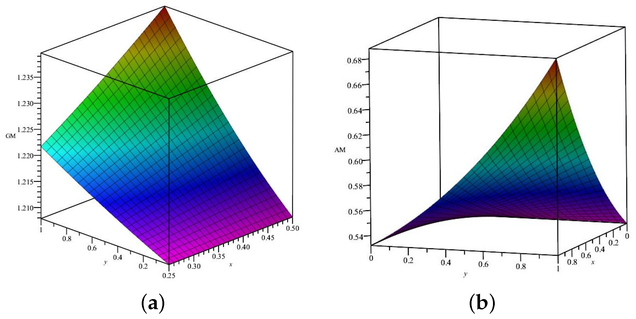
The

Table 1. The values of the aggregation functions.

	$(0.1,0.2)$	$(\frac{1}{4},\frac{1}{8})$	$(\frac{1}{3},\frac{1}{5})$	$(\frac{1}{6},\frac{1}{2})$	$(\frac{1}{7},\frac{2}{11})$
$AM\left(\mathsf{\Phi }\right)$	$0.5338007158$	$0.5379469852$	$0.5347761095$	$0.5394929715$	$0.5343168102$
$GM\left(\mathsf{\Phi }\right)$	$0.07319484539$	$0.08005920524$	$0.07540734458$	$0.08171898282$	$0.07445158788$
$Max\left(\mathsf{\Phi }\right)$	$0.9933555063$	$0.9780228725$	$0.9896373989$	$0.8371284313$	$0.9726044771$
$Min\left(\mathsf{\Phi }\right)$	$0.00008866018283$	$0.0001219787034$	$0.00009892822047$	$0.0001305585469$	$0.00009442854698$
$Med\left(\mathsf{\Phi }\right)$	$0.5708793485$	$0.5868215445$	$0.5746840555$	$0.5926184250$	$0.5728967240$

below shows the different values of the aggregation functions for Ψ.

By comparing the values obtained in the table above, we consider the minimum aggregate function

$$\begin{array}{cc}\hfill \mathrm{diag}& [O{S}_1\left(\mathsf{\Psi }({\omega }_1,\dots ,{\omega }_{\varsigma },\tau )\right),O{S}_1\left(\mathsf{\Psi }({\omega }_1,\dots ,{\omega }_{\varsigma },\tau )\right),\hfill \\ \hfill & O{S}_1\left(\mathsf{\Psi }({\omega }_1,\dots ,{\omega }_{\varsigma },\tau )\right),O{S}_1\left(\mathsf{\Psi }({\omega }_1,\dots ,{\omega }_{\varsigma },\tau )\right)],\hfill \end{array}$$

(27)

as a control function. For $\Theta :\mathit{U}\to \mathit{R}$, we have

$$\begin{array}{cc}\hfill & \mathsf{\Delta }\left({\mathcal{D}}_{\sigma }\Theta ({\omega }_1,\dots ,{\omega }_{\varsigma }),\tau \right)⪰\hfill \\ \hfill \mathrm{diag}& [O{S}_1\left(\mathsf{\Psi }({\omega }_1,\dots ,{\omega }_{\varsigma },\tau )\right),O{S}_1\left(\mathsf{\Psi }({\omega }_1,\dots ,{\omega }_{\varsigma },\tau )\right),\hfill \\ \hfill & O{S}_1\left(\mathsf{\Psi }({\omega }_1,\dots ,{\omega }_{\varsigma },\tau )\right),O{S}_1\left(\mathsf{\Psi }({\omega }_1,\dots ,{\omega }_{\varsigma },\tau )\right)],\hfill \end{array}$$

(28)

$$\begin{array}{cc}\hfill & \mathsf{\Delta }\left(\Theta \left({[{\omega }_1,\dots ,{\omega }_{\varsigma }]}_{\mathit{U}}\right)-{[\Theta \left({\omega }_1\right),\dots ,\Theta \left({\omega }_{\varsigma }\right)]}_{\mathit{R}},\tau \right)⪰\hfill \\ \hfill \mathrm{diag}& [O{S}_1\left(\mathsf{\Psi }({\omega }_1,\dots ,{\omega }_{\varsigma },\tau )\right),O{S}_1\left(\mathsf{\Psi }({\omega }_1,\dots ,{\omega }_{\varsigma },\tau )\right),\hfill \\ \hfill & O{S}_1\left(\mathsf{\Psi }({\omega }_1,\dots ,{\omega }_{\varsigma },\tau )\right),O{S}_1\left(\mathsf{\Psi }({\omega }_1,\dots ,{\omega }_{\varsigma },\tau )\right)],\hfill \end{array}$$

(29)

for all ${\omega }_1,\dots ,{\omega }_{\varsigma }\in \mathit{U}$ and $\sigma \in {\mathit{B}}_{1/{\varsigma }_0}^1$. Then there exists a unique homomorphism $\mathsf{\Omega }:\mathit{U}\to \mathit{R}$ of type ς-LA such that, if $\eta \vartheta <\eta$,

$$\begin{array}{cc}\hfill & \mathsf{\Delta }\left(\Theta \left(\omega \right)-\mathsf{\Omega }\left(\omega \right),\tau \right)⪰\hfill \\ \hfill \mathrm{diag}& [O{S}_1\left(\mathsf{\Psi }({\omega }_1,\dots ,{\omega }_{\varsigma },\tau )\right),O{S}_1\left(\mathsf{\Psi }({\omega }_1,\dots ,{\omega }_{\varsigma },\tau )\right),\hfill \\ \hfill & O{S}_1\left(\mathsf{\Psi }({\omega }_1,\dots ,{\omega }_{\varsigma },\tau )\right),O{S}_1\left(\mathsf{\Psi }({\omega }_1,\dots ,{\omega }_{\varsigma },\tau )\right)],\hfill \end{array}$$

(30)

where

$$\begin{array}{cc}\hfill & \mathsf{\Psi }({\omega }_1,\dots ,{\omega }_{\varsigma },\tau )=\hfill \\ \hfill \mathrm{diag}& [E_{\alpha ,\beta }(\frac{-\parallel \varphi \omega \parallel }{\eta \left({\displaystyle \genfrac{}{}{0pt}{}{\varsigma }{\kappa }}\right)[(\varsigma -\kappa +1)-{(\varsigma -\kappa +1)}^{\vartheta }]\tau }),w_{\sigma ,\upsilon }(\frac{-\parallel \varphi \omega \parallel }{\eta \left({\displaystyle \genfrac{}{}{0pt}{}{\varsigma }{\kappa }}\right)[(\varsigma -\kappa +1)-{(\varsigma -\kappa +1)}^{\vartheta }]\tau }),\hfill \\ & {\mathcal{H}}_{p,q}^{m,n}(\frac{-\parallel \varphi \omega \parallel }{\eta \left({\displaystyle \genfrac{}{}{0pt}{}{\varsigma }{\kappa }}\right)[(\varsigma -\kappa +1)-{(\varsigma -\kappa +1)}^{\vartheta }]\tau }),exp(\frac{-\parallel \varphi \omega \parallel }{\eta \left({\displaystyle \genfrac{}{}{0pt}{}{\varsigma }{\kappa }}\right)[(\varsigma -\kappa +1)-{(\varsigma -\kappa +1)}^{\vartheta }]\tau })],\hfill \end{array}$$

for all $\omega \in \mathit{U}$.

Proof. 

According to inequality (28), we have $\Theta \left(0\right)=0$. In the sequel, by considering

$$\begin{array}{cc}\hfill \mathsf{\Psi }({\omega }_1,\dots ,{\omega }_1,\tau )=\mathrm{diag}& [O{S}_1\left(\mathsf{\Psi }({\omega }_1,\dots ,{\omega }_{\varsigma },\tau )\right),O{S}_1\left(\mathsf{\Psi }({\omega }_1,\dots ,{\omega }_{\varsigma },\tau )\right),\hfill \\ \hfill & O{S}_1\left(\mathsf{\Psi }({\omega }_1,\dots ,{\omega }_{\varsigma },\tau )\right),O{S}_1\left(\mathsf{\Psi }({\omega }_1,\dots ,{\omega }_{\varsigma },\tau )\right)],\hfill \end{array}$$

for all ${\omega }_1,\dots ,{\omega }_{\varsigma }\in \mathit{U}$ and $\lambda ={(\varsigma -\kappa +1)}^{\eta (\vartheta -1)}$ in Theorems 2 and 3, the proof is complete. □

The Figure 1 below shows the different values of the aggregation functions $AM$ and $GM$.

4. H–U–R Stability of Jordan Homomorphisms on $\mathbf{\varsigma }$-LBA

In this section, we investigate the existence of a unique Jordan homomorphism solution and the H–U–R stability of Equation (1).

Theorem 4.

We consider $(\mathit{R},\mathsf{\Delta },⊛)$ and a mapping $\Theta :\mathit{U}\to \mathit{R}$ such that $\Theta \left(0\right)=0$. Then, there exists a function $\mathsf{\Psi }:{\mathit{U}}^{\varsigma }\times (0,+\infty )\to \mathrm{diag}{\mathrm{M}}_{\mathrm{n}}\left((0,1]\right)$ such that

$$\mathsf{\Delta }\left({\mathcal{D}}_{\sigma }\Theta ({\omega }_1,\dots ,{\omega }_{\varsigma }),\tau \right)⪰\mathsf{\Psi }\left({\omega }_1,\dots ,{\omega }_{\varsigma },\tau \right)$$

(31)

$$\mathsf{\Delta }\left(\Theta \left({[\omega \omega \cdots \omega ]}_{\mathit{U}}\right)-{[\Theta \left(\omega \right)\Theta \left(\omega \right)\cdots \Theta \left(\omega \right)]}_{\mathit{R}},\tau \right)⪰\mathsf{\Psi }(\omega ,\omega ,\dots ,\omega ,\tau ),$$

(32)

for all ${\omega }_1,\dots ,{\omega }_{\varsigma }\in \mathit{U}$ and $\sigma \in {\mathit{B}}_{1/{\varsigma }_0}^1$. If there exists $\lambda <1$ satisfying

$$\mathsf{\Psi }({\omega }_1,\dots ,{\omega }_{\varsigma },\tau )⪰\mathsf{\Psi }\left(\frac{{\omega }_1}{\varsigma -\kappa +1},\cdots ,\frac{{\omega }_{\varsigma }}{\varsigma -\kappa +1},\frac{\tau }{(\varsigma -\kappa +1)\lambda }\right),$$

(33)

then there exists a unique Jordan homomorphism $\mathsf{\Omega }:\mathit{U}\to \mathit{R}$ of type ς-LA such that

$$\mathsf{\Delta }\left(\Theta \left(\omega \right)-\mathsf{\Omega }\left(\omega \right),\tau \right)⪰\mathsf{\Psi }\left(\omega ,\omega ,\dots ,\omega ,(\varsigma -\kappa +1)\left(\begin{array}{c}\varsigma \\ \kappa \end{array}\right)(1-\lambda )\tau \right),$$

(34)

for all $\omega \in \mathit{U}$.

Proof. 

In this theorem, too, to begin the proof, as in the previous theorems, we first consider the set $\mathcal{L}$ and then define a meter on this set. The defined metric is along with the $\mathcal{L}$ set of a generalized fuzzy metric space. Next, by considering the mapping $\mathsf{\Lambda }$, the existence of a fixed point such as $\mathsf{\Omega }$ for this mapping is proved. This fixed point is defined as follows

$$\mathsf{\Omega }\left(\omega \right)=\underset{\alpha \to +\infty }{lim}\frac{1}{{(\varsigma -\kappa +1)}^{\alpha }}\Theta \left({(\varsigma -\kappa +1)}^{\alpha }\omega \right),$$

for all $\omega \in \mathit{U}$. In the following, we show that the $\mathbb{C}$-linear mapping $\mathsf{\Omega }$ is a Jordan homomorphism of type $\varsigma$-LA. By (32), we get

$$\begin{array}{cc}\hfill \mathsf{\Delta }(& \mathsf{\Omega }\left({[\omega \omega \cdots \omega ]}_{\mathit{U}}\right)-{[\mathsf{\Omega }\left(\omega \right)\mathsf{\Omega }\left(\omega \right)\cdots \mathsf{\Omega }\left(\omega \right)]}_{\mathit{R}},\tau )\hfill \\ \hfill & =\underset{\alpha \to +\infty }{lim}\mathsf{\Delta }(\Theta \left({[{(\varsigma -\kappa +1)}^{\alpha }\omega {(\varsigma -\kappa +1)}^{\alpha }\omega \cdots {(\varsigma -\kappa +1)}^{\alpha }\omega ]}_{\mathit{R}}\right)\hfill \\ \hfill & -{[\Theta \left({(\varsigma -\kappa +1)}^{\alpha }\omega \right)\Theta \left({(\varsigma -\kappa +1)}^{\alpha }\omega \right)\cdots \Theta \left({(\varsigma -\kappa +1)}^{\alpha }\omega \right)]}_{\mathit{R}},{(\varsigma -\kappa +1)}^{\alpha \varsigma }\tau )\hfill \\ \hfill & ⪰\underset{\alpha \to +\infty }{lim}\mathsf{\Psi }\left({(\varsigma -\kappa +1)}^{\alpha }\omega ,{(\varsigma -\kappa +1)}^{\alpha }\omega ,\dots ,{(\varsigma -\kappa +1)}^{\alpha }\omega ,{(\varsigma -\kappa +1)}^{\alpha \varsigma }\tau \right)=\mathbf{1},\hfill \end{array}$$

for all $\omega \in \mathit{U}$. So

$$\mathsf{\Omega }\left({[\omega \omega \cdots \omega ]}_{\mathit{U}}\right)={[\mathsf{\Omega }\left(\omega \right)\mathsf{\Omega }\left(\omega \right)\cdots \mathsf{\Omega }\left(\omega \right)]}_{\mathit{R}},$$

for all $\omega \in \mathit{U}$. Thus, H–U–R stability of Jordan homomorphism of type $\varsigma$-LA is established. □

In this section, we see similarly that by changing the condition for the control function, the results are still valid, which is shown in the next theorem.

Theorem 5.

We consider $(\mathit{R},\mathsf{\Delta },⊛)$ and a mapping $\Theta :\mathit{U}\to \mathit{R}$ such that $\Theta \left(0\right)=0$. Then, there exists a function $\mathsf{\Psi }:{\mathit{U}}^{\varsigma }\times (0,+\infty )\to \mathrm{diag}{\mathrm{M}}_{\mathrm{n}}\left((0,1]\right)$ such that

$$\mathsf{\Delta }\left({\mathcal{D}}_{\sigma }\Theta ({\omega }_1,\dots ,{\omega }_{\varsigma }),\tau \right)⪰\mathsf{\Psi }\left({\omega }_1,\dots ,{\omega }_{\varsigma },\tau \right)$$

(35)

$$\mathsf{\Delta }\left(\Theta \left({[\omega \omega \cdots \omega ]}_{\mathit{U}}\right)-{[\Theta \left(\omega \right)\Theta \left(\omega \right)\cdots \Theta \left(\omega \right)]}_{\mathit{R}},\tau \right)⪰\mathsf{\Psi }(\omega ,\omega ,\dots ,\omega ,\tau ),$$

(36)

for all ${\omega }_1,\dots ,{\omega }_{\varsigma }\in \mathit{U}$ and $\sigma \in {\mathit{B}}_{1/{\varsigma }_0}^1$. If there exists $\lambda <1$ satisfying

$$\mathsf{\Psi }\left(\frac{{\omega }_1}{\varsigma -\kappa +1},\dots ,\frac{{\omega }_{\varsigma }}{\varsigma -\kappa +1},\tau \right)⪰\mathsf{\Psi }\left({\omega }_1,\dots ,{\omega }_{\varsigma },\frac{(\varsigma -\kappa +1)\tau }{\lambda }\right),$$

(37)

for all ${\omega }_1,\dots ,{\omega }_{\varsigma }\in \mathit{U}$, then there exists a unique Jordan homomorphism $\mathsf{\Omega }:\mathit{U}\to \mathit{R}$ of type ς-LA such that

$$\mathsf{\Delta }\left(\Theta \left(\omega \right)-\mathsf{\Omega }\left(\omega \right),\tau \right)⪰\mathsf{\Psi }\left(\omega ,\omega ,\dots ,\omega ,\frac{(\varsigma -\kappa +1)\left(\begin{array}{c}\varsigma \\ \kappa \end{array}\right)(1-\lambda )\tau }{\lambda }\right),$$

(38)

for all $\omega \in \mathit{U}$.

Proof. 

The proof process is similar to the proof of Theorem 4. □

Example 2.

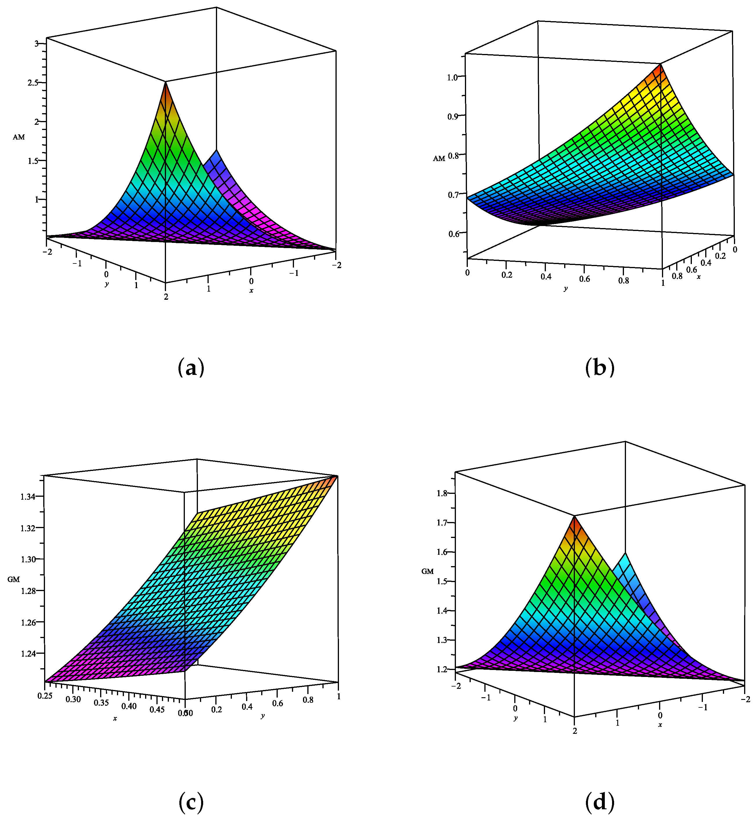
We consider Equation (1), for all ${\omega }_1,\dots ,{\omega }_{\varsigma }\in \mathit{U}$ and $\sigma \in {\mathit{B}}_{1/{\varsigma }_0}^1:=\{exp\left(\mathit{a}ϵ\right);0\le ϵ\le 2\pi {\varsigma }_0\}$ and ${\varsigma }_0\in \mathbb{N}$. Let $\eta \in \{-1,1\}$, $\varphi ,c\in {\mathbb{R}}^{+}$. Consider the function

$$\mathsf{\Psi }({\omega }_1,\dots ,{\omega }_{\varsigma },\tau )=\mathrm{diag}\left[{\mathrm{E}}_{\alpha ,\beta }(\frac{-\parallel \varphi {\sum }_{\mathit{a}=1}^{\varsigma }{\omega }_{\mathit{a}}\parallel }{\tau }),{\mathrm{w}}_{\sigma ,\upsilon }(\frac{-\parallel \varphi {\sum }_{\mathit{a}=1}^{\varsigma }{\omega }_{\mathit{a}}\parallel }{\tau }),{\mathcal{H}}_{p,q}^{m,n}(\frac{-\parallel \varphi {\sum }_{\mathit{a}=1}^{\varsigma }{\omega }_{\mathit{a}}\parallel }{\tau }),exp(\frac{-\parallel \varphi {\sum }_{\mathit{a}=1}^{\varsigma }{\omega }_{\mathit{a}}\parallel }{\tau })\right],$$

(39)

The

Table 2. The values of the aggregation functions.

	$(0.1,0.2)$	$(\frac{1}{4},\frac{1}{8})$	$(\frac{1}{3},\frac{1}{5})$	$(\frac{1}{6},\frac{1}{2})$	$(\frac{1}{7},\frac{2}{11})$
$AM\left(\mathsf{\Phi }\right)$	$0.5628910522$	$0.5955323772$	$0.6019575430$	$0.6180306698$	$0.5659623780$
$GM\left(\mathsf{\Phi }\right)$	$0.09584687750$	$0.1070208793$	$0.1035912864$	$0.1129163606$	$0.09712093981$
$Max\left(\mathsf{\Phi }\right)$	$0.9048374180$	$0.8371284313$	$0.8824969026$	$0.8549297134$	$0.8974255558$
$Min\left(\mathsf{\Phi }\right)$	$0.0002057715410$	$0.0002627425246$	$0.0002255228515$	$0.0002909572644$	$0.0002124668710$
$Med\left(\mathsf{\Phi }\right)$	$0.6732605080$	$0.7723691675$	$0.7036334690$	$0.8355471595$	$0.6831057445$

below shows the different values of the aggregation functions for Ψ.

By comparing the values obtained in the table above, we consider the minimum aggregate function

$$\begin{array}{cc}\hfill \mathrm{diag}& [O{S}_1\left(\mathsf{\Psi }({\omega }_1,\dots ,{\omega }_{\varsigma },\tau )\right),O{S}_1\left(\mathsf{\Psi }({\omega }_1,\dots ,{\omega }_{\varsigma },\tau )\right),\hfill \\ \hfill & O{S}_1\left(\mathsf{\Psi }({\omega }_1,\dots ,{\omega }_{\varsigma },\tau )\right),O{S}_1\left(\mathsf{\Psi }({\omega }_1,\dots ,{\omega }_{\varsigma },\tau )\right)],\hfill \end{array}$$

as a control function.

For $\Theta :\mathit{U}\to \mathit{R}$, we have

$$\begin{array}{cc}\hfill & \mathsf{\Delta }\left({\mathcal{D}}_{\sigma }\Theta ({\omega }_1,\dots ,{\omega }_{\varsigma }),\tau \right)⪰\hfill \\ \hfill \mathrm{diag}& [O{S}_1\left(\mathsf{\Psi }({\omega }_1,\dots ,{\omega }_{\varsigma },\tau )\right),O{S}_1\left(\mathsf{\Psi }({\omega }_1,\dots ,{\omega }_{\varsigma },\tau )\right),\hfill \\ \hfill & O{S}_1\left(\mathsf{\Psi }({\omega }_1,\dots ,{\omega }_{\varsigma },\tau )\right),O{S}_1\left(\mathsf{\Psi }({\omega }_1,\dots ,{\omega }_{\varsigma },\tau )\right)],\hfill \end{array}$$

(40)

$$\begin{array}{cc}\hfill & \mathsf{\Delta }\left(\Theta \left({[\omega ,\cdots ,\omega ]}_{\mathit{U}}\right)-{[\Theta \left(\omega \right),\dots ,\Theta \left(\omega \right)]}_{\mathit{R}},\tau \right)⪰\hfill \\ \hfill \mathrm{diag}& [O{S}_1\left(\mathsf{\Psi }({\omega }_1,\dots ,{\omega }_{\varsigma },\tau )\right),O{S}_1\left(\mathsf{\Psi }({\omega }_1,\dots ,{\omega }_{\varsigma },\tau )\right),\hfill \\ \hfill & O{S}_1\left(\mathsf{\Psi }({\omega }_1,\dots ,{\omega }_{\varsigma },\tau )\right),O{S}_1\left(\mathsf{\Psi }({\omega }_1,\dots ,{\omega }_{\varsigma },\tau )\right)],\hfill \end{array}$$

(41)

where

$$\begin{array}{cc}\hfill \mathsf{\Psi }({\omega }_1,\dots ,{\omega }_{\varsigma },\tau )=\mathrm{diag}& \left[E_{\alpha ,\beta }(\frac{-\parallel \varsigma \varphi \omega \parallel }{\tau }),w_{\sigma ,\upsilon }(\frac{-\parallel \varsigma \varphi \omega \parallel }{\tau }),{\mathcal{H}}_{p,q}^{m,n}(\frac{-\parallel \varsigma \varphi \omega \parallel }{\tau }),exp(\frac{-\parallel \varsigma \varphi \omega \parallel }{\tau })\right],\hfill \end{array}$$

for all ${\omega }_1,\dots ,{\omega }_{\varsigma }\in \mathit{U}$ and $\sigma \in {\mathit{B}}_{1/{\varsigma }_0}^1$. Then there exists a unique Jordan ς-Lie homomorphism $\mathsf{\Omega }:\mathit{U}\to \mathit{R}$ such that, if $\ell c<\eta$,

$$\begin{array}{cc}\hfill & \mathsf{\Delta }\left(\Theta \left(\omega \right)-\mathsf{\Omega }\left(\omega \right),\tau \right)⪰\hfill \\ \hfill \mathrm{diag}& [O{S}_1\left(\mathsf{\Psi }({\omega }_1,\dots ,{\omega }_{\varsigma },\tau )\right),O{S}_1\left(\mathsf{\Psi }({\omega }_1,\dots ,{\omega }_{\varsigma },\tau )\right),\hfill \\ \hfill & O{S}_1\left(\mathsf{\Psi }({\omega }_1,\dots ,{\omega }_{\varsigma },\tau )\right),O{S}_1\left(\mathsf{\Psi }({\omega }_1,\dots ,{\omega }_{\varsigma },\tau )\right)],\hfill \end{array}$$

(42)

for

$$\begin{array}{cc}\hfill \mathsf{\Psi }({\omega }_1,\dots ,{\omega }_{\varsigma },\tau )=\mathrm{diag}& [E_{\alpha ,\beta }(\frac{-\parallel \varsigma \varphi \omega \parallel }{\eta \left(\begin{array}{c}\varsigma \\ \kappa \end{array}\right)[(\varsigma -\kappa +1)-{(\varsigma -\kappa +1)}^c]\tau }),w_{\sigma ,\upsilon }(\frac{-\parallel \varsigma \varphi \omega \parallel }{\eta \left(\begin{array}{c}\varsigma \\ \kappa \end{array}\right)[(\varsigma -\kappa +1)-{(\varsigma -\kappa +1)}^c]\tau }),\hfill \\ \hfill & {\mathcal{H}}_{p,q}^{m,n}(\frac{-\parallel \varsigma \varphi \omega \parallel }{\eta \left(\begin{array}{c}\varsigma \\ \kappa \end{array}\right)[(\varsigma -\kappa +1)-{(\varsigma -\kappa +1)}^c]\tau }),exp(\frac{-\parallel \varsigma \varphi \omega \parallel }{\eta \left(\begin{array}{c}\varsigma \\ \kappa \end{array}\right)[(\varsigma -\kappa +1)-{(\varsigma -\kappa +1)}^c]\tau })].\hfill \end{array}$$

Proof. 

According to inequality (40), we have $\Theta \left(0\right)=0$. In the sequel, by considering

$$\begin{array}{cc}\hfill \mathsf{\Psi }({\omega }_1,\dots ,{\omega }_1,\tau )=\mathrm{diag}& [O{S}_1\left(\mathsf{\Psi }({\omega }_1,\dots ,{\omega }_{\varsigma },\tau )\right),O{S}_1\left(\mathsf{\Psi }({\omega }_1,\dots ,{\omega }_{\varsigma },\tau )\right),\hfill \\ \hfill & O{S}_1\left(\mathsf{\Psi }({\omega }_1,\dots ,{\omega }_{\varsigma },\tau )\right),O{S}_1\left(\mathsf{\Psi }({\omega }_1,\dots ,{\omega }_{\varsigma },\tau )\right)],\hfill \end{array}$$

for all ${\omega }_1,\dots ,{\omega }_{\varsigma }\in \mathit{U}$ and $\lambda ={(\varsigma -\kappa +1)}^{\eta (c-1)}$ in Theorems 4 and 5, the proof is complete. □

The Figure 2 below shows the different values of the aggregation functions $AM$ and $GM$.

References

- Filippov, V.T. On n-Lie algebras. Sib. Mat. Zh. 1985, 26, 126–140. [Google Scholar] [CrossRef]
- Nambu, Y. Generalized Hamiltonian dynamics. Phys. Rev. D 1973, 7, 2405–2412. [Google Scholar] [CrossRef]
- Azcarraga, J.A.; Izquierdo, J.M. n-ary algebras: A review with applications. J. Phys. A 2010, 43, 1–117. [Google Scholar] [CrossRef] [Green Version]
- Bagger, J.; Lambert, N. Comments on multiple M2-branes. J. High Energy Phys. 2008, 2008, 105. [Google Scholar] [CrossRef]
- Filippov, V.T. On n-Lie algebras of Jacobians. Sib. Mat. Zh. 1998, 39, 660–669. [Google Scholar] [CrossRef]
- Ulam, S.M. Problems in Modern Mathematics, Chapter VI, Science ed.; Wiley: New York, NY, USA, 1964. [Google Scholar]
- Aoki, T. On the stability of the linear transformation in Banach spaces. J. Math. Soc. Jpn. 1950, 2, 64–66. [Google Scholar] [CrossRef]
- Rassias, T.M. On the stability of the linear mapping in Banach spaces. Proc. Am. Math. Soc. 1978, 72, 297–300. [Google Scholar] [CrossRef]
- Găvruţxax, P. A generalization of the Hyers-Ulam-Rassias stability of approximately additive mappings. J. Math. Anal. Appl. 1994, 184, 431–436. [Google Scholar] [CrossRef] [Green Version]
- Asgari, G.; Cho, Y.J.; Lee, Y.W.; Gordji, M.E. Fixed points and stability of functional equations in fuzzy ternary Banach algebras. J. Ineq. Appl. 2013, 2013, 166. [Google Scholar] [CrossRef] [Green Version]
- Hassani, F.; Ebadian, A.; Gordji, M.E.; Kenary, H.A. Nearly n-homomorphisms and n-derivations in fuzzy ternary Banach algebras. J. Ineq. Appl. 2013, 2013, 71. [Google Scholar] [CrossRef] [Green Version]
- Rassias, J.M.; Jun, K.W.; Kim, H.M. Approximate (m,n)-Cauchy Jensen Additive Mappings in C*-algebras. Acta Math. Sin. 2011, 27, 1907–1922. [Google Scholar] [CrossRef]
- Rassias, J.M.; Kim, H.M. Generalized Hyers-Ulam stability for general addiitve functional equations in quasi-β-normed spaces. J. Math. Anal. Appl. 2009, 356, 302–309. [Google Scholar] [CrossRef] [Green Version]
- Saxena, R.K. Certain properties of generalized Mittag-Leffler function. In Proceedings of the Third Annual Conference of the Society for Special Functions and Their Applications, Chennai, India, 4–6 March 2002; pp. 75–81. [Google Scholar]
- Mathai, A.M.; Saxena, R.K. The H-Function with Applications in Statistics and Other Disciplines; Halsted Press: Sidney, Australia; John Wiley & Sons: New York, NY, USA; London, UK, 1978; xii+192p, ISBN 0-470-26380-6. [Google Scholar]
- Kilbas, A.A.; Saigo, M. On the H-function. J. Appl. Math. Stoch. Anal. 1999, 12, 191–204. [Google Scholar] [CrossRef] [Green Version]
- Kiryakova, V. Some special functions related to fractional calculus and fractional (non-integer) order control systems and equations. Facta Univ. Ser. Autom. Control Robot. 2008, 7, 79–98. [Google Scholar]
- Eidinejad, Z.; Saadati, R. Hyers-Ulam-Rassias-Wright Stability for Fractional Oscillation Equation. Discret. Dyn. Nat. Soc. 2022, 2022, 2–3. [Google Scholar] [CrossRef]
- Grabisch, M.; Marichal, J.-L.; Mesiar, R.; Pap, E. Aggregation Functions; Encyclopedia of Mathematics and Its Applications, 127; Cambridge University Press: Cambridge, UK, 2009; xviii+460p, ISBN 978-0-521-51926-7. [Google Scholar]
- Klement, E.P.; Mesiar, R.; Pap, E. Triangular norms—Basic properties and representation theorems. In Discovering the World with Fuzzy Logic; Studies in Fuzziness and Soft Computing; Physica: Heidelberg, Germany, 2000; Volume 57, pp. 63–81. [Google Scholar]
- Younis, M.; Sretenovic, A.; Radenovic, S. Some critical remarks on “Some new fixed point results in rectangular metric spaces with an application to fractional-order functional differential equations”. Nonlinear Anal. Model. Control. 2022, 27, 163–178. [Google Scholar] [CrossRef]
- Mitrovic, Z.D.; Dey, L.K.; Radenovic, S. A fixed point theorem of Sehgal-Guseman in bv(s)-metric spaces. Ann. Univ. Craiova Ser. Math. Comput. Sci. 2020, 47, 244–251. [Google Scholar]
- Graily, E.; Vaezpour, S.M.; Saadati, R.; Cho, Y.J. Generalization of fixed point theorems in ordered metric spaces concerning generalized distance. Fixed Point Theory Appl. 2011, 30, 8. [Google Scholar] [CrossRef] [Green Version]
- Brzdek, J.; El-hady, E.; Schwaiger, J. Investigations on the Hyers-Ulam stability of generalized radical functional equations. Aequationes Math. 2020, 94, 575–593. [Google Scholar] [CrossRef] [Green Version]
- Brzdek, J.; Popa, D.; Rasa, I.; Xu, B. Ulam Stability of Operators; Mathematical Analysis and Its Applications; Academic Press: London, UK, 2018. [Google Scholar]
- Shakeri, S.; Ciric, L.J.B.; Saadati, R. Common fixed point theorem in partially ordered L-fuzzy metric spaces. Fixed Point Theory Appl. 2010, 125082. [Google Scholar] [CrossRef] [Green Version]
- Ciric, L.; Abbas, M.; Damjanovic, B.; Saadati, R. Common fuzzy fixed point theorems in ordered metric spaces. Math. Comput. Modelling 2011, 53, 1737–1741. [Google Scholar] [CrossRef]
- Cho, Y.J.; Saadati, R. Lattictic non-Archimedean random stability of ACQ functional equation. Adv. Differ. Equ. 2011, 31, 12. [Google Scholar] [CrossRef] [Green Version]
- Mihet, D.; Saadati, R.; Vaezpour, S.M. The stability of an additive functional equation in Menger probabilistic ϕ-normed spaces. Math. Slovaca 2011, 61, 817–826. [Google Scholar] [CrossRef] [Green Version]
- Cho, Y.J.; Park, C.; Rassias, T.M.; Saadati, R. Stability of Functional Equations in Banach Algebras; Springer: Cham, Switzerland, 2015. [Google Scholar]
- Brzdȩk, J.; Fošner, A. Remarks on the stability of Lie homomorphisms. J. Math. Anal. Appl. 2013, 400, 585–596. [Google Scholar] [CrossRef]
- Gordji, M.E.; Khodaei, H. A fixed point technique for investigating the stability of (α,β,γ)-derivations on Lie C*-algebras. Nonlinear Anal. 2013, 76, 52–57. [Google Scholar] [CrossRef]
- Diaz, J.B.; Margolis, B. A fixed point theorem of the alternative for contractions on a generalized complete metric space. Bull. Am. Math. Soc. 1968, 74, 305–309. [Google Scholar] [CrossRef] [Green Version]
- Hyers, D.H.; Isac, G.; Rassias, T.M. Stability of Functional Equations in Several Variables; Birkhäuser: Boston, MA, USA, 1998. [Google Scholar]
- Jung, S.M. Hyers-Ulam-Rassias Stability of Functional Equations in Nonlinear Analysis; Springer Science: New York, NY, USA, 2011. [Google Scholar]
- Kannappan, P. Functional Equations and Inequalities with Applications; Springer Science: New York, NY, USA, 2009. [Google Scholar]
- Lu, G.; Xie, J.; Liu, Q.; Yuanfeng, J. Hyers-Ulam stability of derivations in fuzzy Banach space. J. Nonlinear Sci. Appl. 2016, 9, 5970–5979. [Google Scholar] [CrossRef] [Green Version]
- Pansuwan, A.; Sintunavarat, W.; Choi, J.Y.; Cho, Y.J. Ulam-Hyers stability, well-posedness and limit shadowing property of the fixed point problems in M-metric spaces. J. Nonlinear Sci. Appl. 2016, 9, 4489–4499. [Google Scholar] [CrossRef] [Green Version]
- Park, C.; Kim, S.O.; Alaca, C. Stability of additive-quadratic ρ-functional equations in Banach spaces: A fixed point approach. J. Nonlinear Sci. Appl. 2017, 10, 1252–1262. [Google Scholar] [CrossRef] [Green Version]
- Rassias, T.M. Functional Equations, Inequalities and Applications; Kluwer Academic: Dordrecht, The Netherlands, 2003. [Google Scholar]
- Sahoo, P.K.; Kannappan, P. Introduction to Functional Equations; CRC Press: Boca Raton, FL, USA, 2011. [Google Scholar]
- Shen, Y. An integrating factor approach to the Hyers-Ulam stability of a class of exact differential equations of second order. J. Nonlinear Sci. Appl. 2016, 9, 2520–2526. [Google Scholar] [CrossRef] [Green Version]
- Zhou, M.; Liu, X.-L.; Cho, Y.J.; Damjanovic, B. Ulam-Hyers stability, well-posedness and limit shadowing property of the fixed point problems for some contractive mappings in Ms-metric spaces. J. Nonlinear Sci. Appl. 2017, 10, 2296–2308. [Google Scholar] [CrossRef] [Green Version]
- Eidinejad, Z.; Saadati, R.; de la Sen, M. Radu-Mihet Method for the Existence, Uniqueness, and Approximation of the ψ-Hilfer Fractional Equations by Matrix-Valued Fuzzy Controllers. Axioms 2021, 10, 63. [Google Scholar] [CrossRef]
Figure 1.
Graphs related to the aggregation functions and for different values. (a) ; (b) .
Figure 2.
Graphs (a–d) are related to the aggregation functions and for different values. (a) ; (b) ; (c) ; (d) .