
An Extended ORESTE Approach for Evaluating Rockburst Risk under Uncertain Environments

1
School of Resource Environment and Safety Engineering, University of South China, Hengyang 421001, China
2
College of Physics and Optoelectronic Engineering, Shenzhen University, Shenzhen 518000, China
3
School of Resources and Safety Engineering, Central South University, Changsha 410083, China
*
Authors to whom correspondence should be addressed.
Mathematics 2022, 10(10), 1699; https://doi.org/10.3390/math10101699
Submission received: 10 April 2022
/
Revised: 12 May 2022
/
Accepted: 13 May 2022
/
Published: 16 May 2022
(This article belongs to the Special Issue Applications of Fuzzy Modeling in Risk Management)
Abstract
:Rockburst is a severe geological disaster accompanied with the violent ejection of rock debris, which greatly threatens the safety of underground workers and equipment. This study aims to propose a novel multi-criteria decision-making (MCDM) approach for evaluating rockburst risk under uncertain environments. First, considering the heterogeneity of rock mass and complexity of geological environments, trapezoidal fuzzy numbers (TrFNs) are adopted to express initial indicator information. Thereafter, the superiority linguistic ratings of experts and a modified entropy weights model with TrFNs are used to calculate the subjective and objective weights, respectively. Then, comprehensive weights can be determined by integrating subjective and objective weights based on game theory. After that, the organísation, rangement et synthèse de données relarionnelles (ORESTE) approach is extended to obtain evaluation results in a trapezoidal fuzzy circumstance. Finally, the proposed approach is applied to assess rockburst risk in the Kaiyang phosphate mine. In addition, the evaluation results are compared with empirical methods and other trapezoidal fuzzy MCDM approaches. Results show that the proposed extended ORESTE approach is reliable for evaluating rockburst risk, and provides an effective reference for the design of prevention techniques.
Keywords:
rockburst; trapezoidal fuzzy numbers (TrFNs); organísation; rangement et synthèse de données relarionnelles (ORESTE); risk evaluation; comprehensive weightsMSC:
90B50; 94D051. Introduction
The mining industry is vital for human survival and social progress, since it provides abundant raw materials for other industries [1]. With the depletion of shallow mineral resources, mining depths are becoming deeper and deeper [2]. However, some challenges still exist when excavating in deep mines. One of the most important concerns is rockburst disasters induced by the instantaneous release of elastic strain energy [3]. As a rockburst is often accompanied by a violent ejection of rock debris, the safety of underground workers and equipment is greatly threatened. For example, a violent rockburst happened in the Klerksdorp district of South Africa, resulting in two deaths and fifty-eight injuries [4]; and an intense rockburst with a Richter scale of 3.5 occurred in the Falconbridge mine, which caused four deaths and the collapse of massive amounts of rock [5]. Due to its serious consequences, evaluating rockburst risk effectively is essential and plays a significant role in risk management for deep mines.
Many methods have been proposed to evaluate rockburst risk, which can be mainly summarized as on-site monitoring techniques, empirical criteria, numerical simulation methods, machine-learning algorithms and multi-criteria decision-making (MCDM) approaches. Among them, on-site monitoring techniques are the most-direct method to determine rockburst risk. Many monitoring technologies are adopted to detect risk warning signs, which include the drilling cutting method [6], the electromagnetic radiation technique [7], acoustic emissions technology [8] and the microseismic monitoring technique [9]. Although the monitoring results are valid, the relationship between monitoring data and rockburst risk is hard to determine, and the operation is complicated and time-consuming. Based on the understanding of rockburst mechanisms and field experience, many empirical criteria have been summarized, including Russenes’s criterion [10], Barton’s criterion [11], Turchaninov’s criterion [12], Kidybinski’s criterion [13], and so on [14,15]. Although empirical criteria are simple and easy to understand, the risk evaluation results may be dissimilar or even contradictory, according to different field experiences. Due to the rapid development of rock mechanics and simulation software, numerical simulation methods have become effective means to determine rockburst risk. The core of such methods is to establish the quantitative relationship between rockburst risk and numerical indicators. Many indicators, such as energy-release rate [16], local energy-release rate [17], burst-tendency index [18], rockburst energy-release rate [19] and failure-approaching index [20], have been proposed. According to their spatial distribution, the rockburst risk in different locations can be effectively determined. Although numerical simulation methods can simultaneously consider the influence of in-situ stress, rock parameters and excavation activities, the model inputs and constitutive relations are difficult to precisely determine. With the accumulation of rockburst data, many machine-learning algorithms have been used to analyze rockburst risk, which include Bayesian networks [21], logistic regression [22], support vector machine [23], ensemble learning [24], and so on [25,26]. Although machine-learning algorithms can well handle nonlinear problems, plenty of reliable data is needed to improve their predictive performance. Considering that rockburst is affected by numerous factors, MCDM technologies have become popular to assess its risk. Some typical MCDM approaches include the technique for order preference by similarity to ideal solution (TOPSIS) [27], the fuzzy matter-element model [28], an acronym in Portuguese of interactive and multiple attribute decision-making (TODIM) [29], and so on [30]. MCDM approaches can not only consider the comprehensive influence of multiple factors, but also deal with uncertainty issues by combing fuzzy theory. However, the indicator weights and grading standard of rockburst risk need to be determined.
Due to the heterogeneity of rock mass and complexity of geological environments, a single crisp number cannot sufficiently indicate the inherent variability in indicator values. Under this circumstance, the indicator information of rockburst risk is hard to accurately denote by crisp numbers. Considering that a fuzzy set can be used to express uncertain and imprecise information, it may be an appropriate way to indicate the indicator values. Although different types of methods have their own advantages, MCDM approaches are preferentially selected in this study. A primary reason is that they can be extended with fuzzy theory to solve uncertain problems. In this case, two key problems should be solved. The first one is the selection of the fuzzy set. Since Zadeh [31] pioneered the idea of fuzzy set theory, many extensions of fuzzy sets have been proposed to solve fuzzy decision issues. Among them, triangular fuzzy numbers and trapezoidal fuzzy numbers (TrFNs) are commonly used. Considering triangular fuzzy numbers are special cases of TrFNs, TrFNs are selected to describe assessment information of rockburst risk under uncertain conditions. As a typical fuzzy set, TrFNs are simple and effective, and have been widely applied in multiple fields, such as supplier selection [32], service-quality evaluation [33] and manufacturing-firm-performance measurement [34].
The second problem is the selection of MCDM approaches. In addition to the used rockburst risk assessment methods, the organísation, rangement et synthèse de données relarionnelles (ORESTE) is an another effective MCDM approach to deal with risk evaluation problems [35]. The reason is two-fold. First, it is proposed based on the general formulation of pairwise comparative rules, and can acquire a reliable rank. Second, a clear advantage of this method is that it can identify concrete relations (such as preference, indifference and incomparability) among alternatives, and then obtain more-comprehensive relationships of alternatives [36]. In recent years, it has received extensive attentions and been used in many fields. For example, Wang et al. [37] adopted a double hierarchy hesitant fuzzy linguistic ORESTE method to assess traffic congestion; Kaya [38] integrated the Gaussian membership function and ORESTE method to monitor brand performance; Liu et al. [39] proposed an integrated TOPSIS–ORESTE framework for new-energy-investment assessment; Liang and Li [40] combined qualitative flexible (QUALIFLEX) and ORESTE techniques to assess the performance of green mines under hesitant fuzzy environments; and Adali and IŞIK [41] utilized the ORESTE approach to obtain the ranking results of web-design firms. Therefore, there is the potential to assess rockburst risk by extending the ORESTE method with TrFNs.
This study intends to propose a novel MCDM framework for the evaluation of rockburst risk. First, the methodology is established by integrating TrFNs, the combination weighting method and an extended ORESTE approach. Then, the proposed approach is used to evaluate the rockburst risk of different lithologies in the Kaiyang phosphate mine. Finally, the effectiveness is verified by comparing with empirical methods and other MCDM approaches.
2. Methodology
An extended ORESTE approach with TrFNs for the risk evaluation of rockburst is proposed in this section. First, the preliminaries of TrFNs are introduced. Then, the procedures of extended ORESTE method are elaborated.
2.1. Trapezoidal Fuzzy Numbers
(1) The definition of TrFNs
A trapezoidal fuzzy number (TrFN) is expressed as , which can be described in Figure 1. The membership function is defined as [42]:
where ; and represent the smallest and largest possible values, respectively; and the interval denotes the most-promising possible values.
(2) Arithmetic operations
Suppose and are two arbitrary TrFNs, and is a positive real number; then, the arithmetic operations can be determined as [43]:
(3) The distance between two TrFNs
According to [44], the generalized distance of fuzzy numbers is a non-negative function with two parameters p and q. Furthermore, q = 1/2 is suggested when there is no reason for distinguishing any side of fuzzy numbers, and p = 2 is more useful in the calculating process. As a result, when p = 2 and q = 1/2, the distance between two TrFNs and can be calculated by [44]:
(4) The comparison method between two TrFNs
The idea of the center of area method is introduced to transform TrFNs into crisp values. As a widely used approach, the center of area method is easy to understand and operate. Compared with other defuzzification techniques, the largest advantages of this method are that it can greatly reduce number of calculations and amount of memory space. Based on the center of area method, the TrFN can be transformed into corresponding crisp number. The transfer formula is [32]:
Then, the comparison method of TrFNs can be determined by:
2.2. Extended ORESTE Method
An extended ORESTE method with TrFNs is proposed in this section, as shown in Figure 2. This methodology integrates TrFNs, combination weighting method and ORESTE approach simultaneously. It includes three phases: express the evaluation information using TrFNs, determine the indicator weights, and obtain the evaluation results with extended ORESTE method. First, TrFNs are adopted to express initial indicator values, so that the ambiguous information can be well indicated. Then, a combination weighting method, which integrates the subjective and objective weights based on game theory, is used to calculate the indicator weights. Finally, the ORESTE approach is extended by TrFNs to determine the risk level of rockburst. The detailed process is indicated as follows.
(1) Phase 1: express the evaluation information using TrFNs
Step 1: Obtain the initial indicator values.
According to laboratory tests and field investigation, the initial indicator values can be obtained, which are expressed as:
where is a crisp number, which indicates the value of alternative (which refers to the rock mass in different areas in this study) for indicator .
Step 2: Normalize the initial decision-making matrix.
Considering the dimensions and units of indicators are different, the initial matrix should be normalized. To normalize the indicator values within 0 and 1, a common normalized technique, the max–min normalization method, is adopted. The largest advantages of this method are that it is independent of the size or amount of dataset.
For benefit indicators, the normalization value can be obtained by [45]:
For cost indicators, the standardized value can be determined by [45]:
Step 3: Convert the indicator values into TrFNs.
Due to the anisotropy and heterogeneity of rock mass, the quantitative indicator values are susceptible to uncertainty. Therefore, this study introduces two parameters to convert crisp numbers into TrFNs, so that the uncertainty can be captured. The conversion formula is:
where and indicate the uncertainty parameters, and .
This means the most-promising possible values are in the interval , the less likely are in the intervals and , and the impossible in the intervals and . Comparing with a single crisp number , the transformed TrFNs can reflect the real situation better.
Then, the fuzzy matrix can be denoted as:
(2) Phase 2: determine the indicator weights
Step 1: Calculate the subjective weights.
The subjective weights are calculated by superiority linguistic ratings of experts. Linguistic variables, such as “very low” and “high”, are adopted to describe the importance of indicators. These linguistic variables are then transformed into the corresponding TrFNs. The relationship between linguistic terms and TrFNs can be consulted in [46].
After all experts give the linguistic ratings, the aggregated weight can be calculated as:
where indicates the weight of indicator given by expert .
Based on Equation (8), the subjective weights can be obtained by:
where is the transformation formula defined in Equation (8), namely,
Step 2: Compute the objective weights.
The entropy weights model corresponding to TrFNs is used to calculate the objective weights. Since Shannon [47] first proposed the concept of entropy to measure the amount of information, the entropy value of decision-making matrix is widely used to calculate indicator weights [31]. The calculation procedure is demonstrated as follows.
The entropy value is determined by:
where .
Then, the objective weights can be calculated by:
Step 3: Determine the comprehensive weights.
The comprehensive weights are determined by integrating subjective and objective weights according to game theory. The purpose is to seek a compromise between comprehensive and basic weights so that their deviation is minimized. Suppose the basic weight vector is:
where , and indicates the numbers of weight vector obtained by different methods.
The arbitrary linear combination of different weight vector is:
where is the combination coefficient and is the comprehensive weight vector set.
To make the deviation between and minimized, should be optimized. The gaming model is established as:
The optimal first derivative of Equation (21) is:
The matrix form of Equation (22) is:
After is calculated, it can be normalized by:
Then, the comprehensive weights are calculated by:
(3) Phase 3: obtain the evaluation results with the extended ORESTE method
Step 1: Compute the significance degree.
First, determine the positive ideal solution and the negative ideal solution under each indicator.
Thereafter, the significance degree of alternative under indicator is computed with
Step 2: Calculate the global preference score.
Given a coefficient , then the global preference score of each alternative under each indicator can be obtained with
Step 3: Determine the weak rank of alternatives.
The preference score of alternative is
According to the value of , the weak rank of alternatives are derived. That is, the bigger the value of , the better the alternative .
Step 4: Calculate the average preference intensity and the net preference intensity.
The average preference intensity of to can be computed with
Thus, the net preference intensity of to can be calculated with
Step 5: Build the preference/indifference/incomparability (PIR) structure.
First, the rules of the indifference and incomparability test (namely, the conflict analysis) are defined as follows:
- (1)
- When , then ;
- (2)
- When , then , where and are two parameters.
For determining the values of and , the following approach can be utilized.
According to the literature [36], if , then and can be regarded as indifferent. On the other hand, they are regarded as indifferent if their distance , where is a threshold. Suppose , then . As a result, let . For the P relation : , so the trapezoidal fuzzy preference threshold can be computed with ; for the R relation : and should be met under at least one indicator. Therefore, for the I relation , the trapezoidal fuzzy incomparability threshold can be calculated with .
Step 6: Obtain the strong rank of alternatives.
The strong rank of alternative is attained according to the weak rank and the PIR structure. Specifically, based on the P and I relations in the PIR structure, the rank of some alternatives is firstly determined, and then the full rank can be derived by combing the weak rank when the R relations exist among other alternatives. For instance, if the weak rank of four alternatives is , and the PIR relations contain: , , , , and , then, according to the P and I relations in the PIR structure, the rank of part of alternatives is firstly determined. Namely, because , because , because , because and because , while the rank of alternatives and cannot be directly determined by the PIR relations because . In this case, the weak rank of alternatives and can be taken as a reference. As is in the weak rank, the full rank of alternatives can be derived as . That is, the strong rank is .
3. Case Study
3.1. Project Profile
The Kaiyang phosphate mine is located in Jinzhong Town, Guiyang City, Guizhou Province, as shown in Figure 3. It is an extra-large phosphate mine with a history of more than sixty years, and contains four sections (namely, Maluping, Qincaichong, Yongshaba and Shabatu). The lithology of this mine is mainly composed of dolomite, phosphate ore, sandstone and red shale. With the increase in mining depth, the geological conditions become more complicated and the ground stress elevates significantly, resulting in an increase in rockburst risk. Several rockbursts have occurred in the Kaiyang phosphate mine, which pose a great threat to personnel safety and seriously affect the production. Therefore, it is necessary to evaluate the rockburst risk in different lithologies, which is valuable for personnel exposure management and the design of prevention techniques.
3.2. Determination of Evaluation Indicators
In order to comprehensively reflect the influence factors of rockburst, five indicators, including the rock-brittleness coefficient (), elastic-energy index (), linear elastic energy (), ground-stress index () and rock-mass-integrity coefficient () are adopted. Among them, indicates the degree of rock brittleness, which can be calculated by:
where is the unconfined compressive strength, and is the tensile strength.
indicates the proportion of energy accumulation and dissipation, which can be calculated by:
where is the stored elastic energy, and is the dissipated energy.
indicates the magnitude of elastic energy, which can be calculated by:
where is the unloading tangential modulus.
indicates the intensity of ground stress, which can be calculated by:
where is the maximum horizontal principle stress.
indicates the integrity of rock mass, which can be calculated by:
where and are the elastic wave speeds of rock mass and rock, respectively.
3.3. Risk Evaluation of Rockburst
In Phase 1, the initial indicator values were obtained. To determine the rockburst risk in different lithologies, dolomite, phosphate ore, red shale and sandstone were adopted for assessment. These alternatives were denoted as , , and , respectively.
Based on laboratory tests and in-situ stress measurement, the initial indicator values were calculated, which were listed in Table 2. Meanwhile, the samples with known levels were obtained based on Table 1, so that the risk levels of each alternative could be determined. The samples with level , , and were indicated as , , and , respectively, as shown in Table 2.
Next, the initial indicator values were normalized. As and are cost indicators, their normalization values were calculated based on Equation (12). Meanwhile, , and are benefit indicators, so their normalization values were determined according to Equation (11). The normalized decision-making matrix is shown in Table 3.
According to Equation (13), the indicator values were converted into TrFNs. In this study, the uncertainty parameters and were, respectively, selected as 0.1 and 0.2. Therefore, the fuzzy decision-making matrix with TrFNs was established, as in Table 4.
In Phase 2, the indicator weights were determined. First, subjective weights were calculated by superiority linguistic ratings. Five experts were invited to give the linguistic ratings of indicators, as indicated in Table 5. These linguistic ratings were transformed into TrFNs, and the aggregated TrFNs were calculated by Equation (15) (see the third column in Table 5). The subjective weights were obtained by Equation (16) (see the fourth column in Table 5).
Then, the extended entropy weights model was used to calculate objective weights. Based on Equation (17), the entropy value of each criterion was calculated as: . According to (18), the subjective weights were determined as: .
Finally, the comprehensive weights were determined based on game theory. By using Equations (23) and (24), the combination coefficient was calculated as: . Based on Equation (25), the comprehensive weights were determined as: .
In Phase 3, the extended ORESTE method was used to obtain the ranking results. First, based on Equation (9), the positive solution of each indicator was: , and the negative solution of each indicator was: . Then, according to Equation (26), the significance degree was determined, as in Table 6.
Suppose , the global preference score was calculated using Equation (27), as shown in Table 7.
Based on Equation (28), the preference scores were calculated as: , , , , , , , and .
As , the weak rank of each alternative was determined as: .
According to Equation (29), the average preference intensity was calculated, as in Table 8.
The net preference intensity was determined by Equation (30), as shown in Table 9.
Considering a representative condition, namely, and , then . Thus, , and . Thereafter, the PIR structure of alternatives was established, as in Table 10.
According to the PIR structure in Table 10, the strong rank order was determined as: . Therefore, the risk of belonged to level to , the risk of and was level , and the risk of was level .
4. Discussions
4.1. Comparison Analysis
To further verify the effectiveness of the proposed methodology, some empirical methods and other MCDM approaches were adopted as comparisons.
First, empirical methods were adopted to determine the rockburst risk. The evaluation results of empirical methods are indicated in Table 11. It can be seen that the evaluation results of different empirical methods were dissimilar, and some of them were even contradictory. The reason may be that these empirical methods were proposed only from one aspect, whereas the rockburst is affected by numerous factors, such as ground stress, rock strength and energy storage capacity. Therefore, it is more reasonable to assess the rockburst risk by considering multiple factors simultaneously. In addition, although the empirical methods were simple and easy to use, the specific rank of different alternatives cannot be obtained.
Subsequently, some other MCDM methods based on TrFNs were used to compare with the proposed method. The evaluation results are shown in Table 12. The specific calculation process was indicated as follows.
When the trapezoidal fuzzy TOPSIS method [44] was used, the weighted decision matrix was first obtained. Then, the positive ideal solutions were determined as: , , , , ; and all of the negative ideal solutions were determined as: . After that, the distances from the positive ideal solution were calculated as: , and the distances from the negative ideal solution were calculated as: . The relative closeness of each alternative was: . As , the ranking result was .
When using the trapezoidal fuzzy TODIM method [51], the partial dominance matrix was first obtained. Then, the dominance matrix of each alternative over other alternatives was:
After that, the global values were: , , , , , , and . As , the ranking result was .
Based on Table 12, it can be seen that the weak rank of the proposed approach was the same as the ranking result of the trapezoidal fuzzy TOPSIS method, and there was a small difference with that of the trapezoidal fuzzy TODIM method. Specifically, only the ranks of and were reversed. However, according to the strong rank of the proposed method, the ranks of , and were almost consistent. In addition, the rank of alternatives , , and was always , and the rank of , , and was always . Therefore, it indicated that the evaluation result of the proposed methodology was reliable and effective.
4.2. Sensitivity Analysis
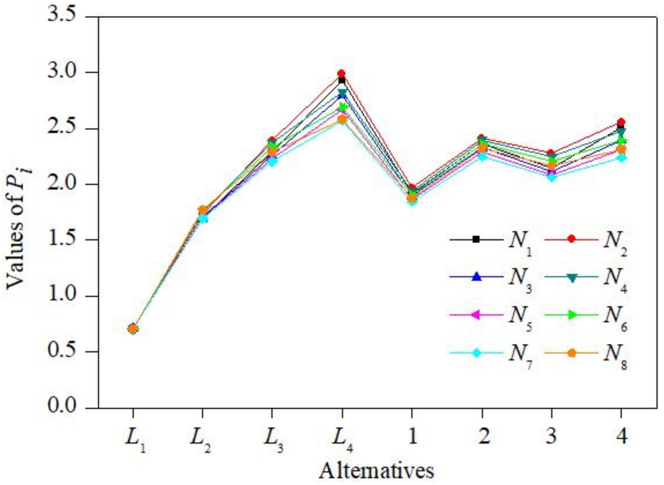
In this study, the values of uncertainty parameters and in Equation (13) were suggested as 0.1 and 0.2, respectively. However, due to differences in the understanding of rockburst and the reliability of data sources, the values of and may be various. To explore the effect of parameter values on the results, other and values were selected. The evaluation results of different and values are shown in Table 13. It can be seen that the weak ranks under dissimilar circumstances were the same. However, it did not mean that the uncertainty parameters had no effect on the results. The preference score of each alternative was calculated, as shown in Figure 4. The trends of values were variant, which indicated that uncertainty parameters may cause changes in evaluation results. In addition, the strong ranks under different and values had some small differences. However, the overall evaluation results was relatively stable.
In addition, considering that the uncertainty of different indicators may not be equal, different values of and for each indicator were chosen, and the evaluation results are shown in Table 14. From Table 14, it can be seen that the weak ranks of , , , , and were consistent, and the weak ranks of and were the same. However, the ranks of and were different. The preference score of each alternative was calculated, which are displayed in Figure 5. The trend of for different alternatives was different, resulting in the difference of rank. Moreover, the strong rank under different values of and for each indicator were not the same. Therefore, it can be concluded the values of uncertainty parameters for each indicator have a certain influence on the evaluation results.
Based on the results of sensitivity analysis, the values of uncertainty parameters affect the evaluation results directly. In reality, the uncertainty parameters can be determined according to the variability in indicator values and the quality of data. To obtain more reliable uncertainty parameters, multiple experiments can be conducted to acquire more indicator values. Then, the distribution and variability of data can be used to determine the preliminary uncertainty parameter values. After that, a sensitivity analysis can be conducted to obtain the final value according to the changes in results. It should be noted that the values of uncertainty parameters depend on the specific application.
4.3. Managerial Implication
According to the evaluation results, some managerial implications can be obtained to manage the rockburst risk in mines.
- (1)
- Due to the influence of uncertainty on the evaluation results, some measures should be taken to avoid uncertainty in reality, such as ensuring the high quality of data.
- (2)
- Based on the evaluation results, the areas of high risk should receive more attention. For example, a monitoring system can be installed for the early warning of rockburst.
- (3)
- The technical parameters of rockburst prevention measures can be optimized according to different risk levels. For different risk levels, the prevention measures and their parameters should be different.
To sum up, this study enriches the representation of uncertain information of rockburst indicators, the determination of indicator weights, and the evaluation methods of rockburst risk. The highlights of the presented methodology are summarized as follows:
- (1)
- The indicator values were expressed by TrFNs after the uncertainty parameters were introduced, which can indicate the uncertain information more reasonably.
- (2)
- Game theory was used to calculate the indicator weights by combining subjective and objective weights, so that the comprehensive weights can be determined more credibly.
- (3)
- The ORESTE approach was extended with TrFNs, which can be used to solve MCDM problems under trapezoidal fuzzy environments.
- (4)
- The proposed methodology was applied to evaluate rockburst risk, and can obtain evaluation results reliably.
5. Conclusions
Evaluating rockburst risk is a crucial issue for the safe and efficient mining in deep mines. This study proposed an extended ORESTE approach with TrFNs to assess rockburst risk. Considering the uncertainty of evaluation information, TrFNs were adopted to express the indicator values. The subjective and objective weights were calculated by the superiority linguistic ratings of experts and a modified entropy weights model, respectively. The final indicator weights were determined by integrating subjective and objective weights based on game theory. To obtain the evaluation results under a fuzzy environment, an extended ORESTE approach was proposed based on TrFNs. The proposed methodology was applied to evaluate the rockburst risk of different lithologies in the Kaiyang phosphate mine. By comparing the evaluation results with empirical methods and other trapezoidal fuzzy MCDM approaches, it indicated that the proposed methodology was reliable and feasible. The evaluation results provided an effective guidance for personnel-exposure management and the prevention of rockburst.
TrFNs enrich the representation of uncertain information in mining and geotechnical engineering, and they can be used to express other similar evaluation information in the future. The proposed methodology can also be adopted to handle other fuzzy MCDM issues, such as landslide risk analysis, tunnel stability evaluation and rock-mass quality classification. In addition, the determination of uncertainty parameters is worth researching in depth.
Author Contributions
Conceptualization, K.S. and Y.L.; methodology, W.L.; validation, K.S., Y.L. and W.L.; investigation, W.L.; writing—original draft preparation, K.S.; writing—review and editing, Y.L. and W.L.; supervision, Y.L.; funding acquisition, Y.L. All authors have read and agreed to the published version of the manuscript.
Funding
This research was funded by the Research and Development Program in Key Areas of Hunan Province (No. 2019SK2011), the Hunan Provincial Innovation Foundation for Postgraduate (No. CX20190711), the National Natural Science Foundation of China (No. 11875164), and the National Defense Military Industry Project of China (No. JSZL2019403C001).
Institutional Review Board Statement
Not applicable.
Informed Consent Statement
Not applicable.
Data Availability Statement
Not applicable.
Conflicts of Interest
The authors declare no conflict of interest.
References
- Ali, S.H.; Giurco, D.; Arndt, N.; Nickless, E.; Brown, G.; Demetriades, A.; Durrheim, R.; Enriquez, M.A.; Kinnaird, J.; Littleboy, A.; et al. Mineral supply for sustainable development requires resource governance. Nature 2017, 543, 367–372. [Google Scholar] [CrossRef]
- Ranjith, P.G.; Zhao, J.; Ju, M.; De Silva, R.V.; Rathnaweera, T.D.; Bandara, A.K. Opportunities and challenges in deep mining: A brief review. Engineering 2017, 3, 546–551. [Google Scholar] [CrossRef]
- Li, D.Y.; Liu, Z.D.; Armaghani, D.J.; Xiao, P.; Zhou, J. Novel ensemble tree solution for rockburst prediction using deep forest. Mathematics 2022, 10, 787. [Google Scholar] [CrossRef]
- Durrheim, R.J. Mitigating the risk of rockbursts in the deep hard rock mines of South Africa: 100 years of research. In Extracting the Science: A Century of Mining Research; Brune, J., Ed.; Society for Mining, Metallurgy, and Exploration: Littleton, CO, USA, 2010; pp. 156–171. [Google Scholar]
- Hedley, D.G.F. A Five-Year Review of the Canada–Ontario Industry Rockburst Project; Special Report SP90; Division Report SP90-064; Canada Centre for Mineral and Energy Technology, Mining Research Laboratory: Ottawa, ON, Canada, 1990. [Google Scholar]
- Shan, Q.Y.; Qin, T. The improved drilling cutting method and its engineering applications. Geotech. Geol. Eng. 2019, 37, 3715–3726. [Google Scholar] [CrossRef]
- Wang, E.Y.; He, X.Q.; Wei, J.P.; Nie, B.S.; Song, D.Z. Electromagnetic emission graded warning model and its applications against coal rock dynamic collapses. Int. J. Rock Mech. Min. Sci. 2011, 48, 556–564. [Google Scholar] [CrossRef]
- Zhou, X.P.; Peng, S.L.; Zhang, J.Z.; Qian, Q.H.; Lu, R.C. Predictive acoustical behavior of rockburst phenomena in Gaoligongshan tunnel, Dulong river highway, China. Eng. Geol. 2018, 247, 117–128. [Google Scholar] [CrossRef]
- Ullah, B.; Kamran, M.; Rui, Y.C. Predictive modeling of short-term rockburst for the stability of subsurface structures using machine learning approaches: T-SNE, K-Means clustering and XGBoost. Mathematics 2022, 10, 449. [Google Scholar] [CrossRef]
- Russenes, B.F. Analysis of Rock Spalling for Tunnels in Steep Valley Sides; Department of Geology, Norwegian Institute of Technology: Trondheim, Norway, 1974. [Google Scholar]
- Barton, N.; Lien, R.; Lunde, J. Engineering classification of rock masses for the design of tunnel support. Rock Mech. Rock Eng. 1974, 6, 189–236. [Google Scholar] [CrossRef]
- Turchaninov, I.A.; Markov, G.A.; Gzovsky, M.V.; Kazikayev, D.M.; Frenze, U.K.; Batugin, S.A.; Chabdarova, U.I. State of stress in the upper part of the earth’s crust based on direct measurements in mines and on tectonophysical and seismological studies. Phys. Earth Planet. Inter. 1972, 6, 229–234. [Google Scholar] [CrossRef]
- Kidybiński, A. Bursting liability indices of coal. Int. J. Rock Mech. Min. Sci. Geomech. Abstr. 1981, 18, 295–304. [Google Scholar] [CrossRef]
- Lee, S.M.; Park, B.S.; Lee, S.W. Analysis of rockbursts that have occurred in a waterway tunnel in Korea. Int. J. Rock Mech. Min. Sci. 2004, 41, 911–916. [Google Scholar] [CrossRef]
- Tao, Z.Y. Support design of tunnels subjected to rockbursting. In Proceedings of the International Society for Rock Mechanics and Rock Engineering International Symposium, Madrid, Spain, 12–16 September 1988. [Google Scholar]
- Cook, N.G.W.; Hoek, E.; Pretorius, J.P.; Ortlepp, W.D.; Salamon, M.D.G. Rock mechanics applied to study of rockbursts. J. S. Afr. Inst. Min. Metall. 1966, 66, 435–528. [Google Scholar]
- Su, G.S.; Feng, X.T.; Jiang, Q.; Chen, G.Q. Study on new index of local energy release rate for stability analysis and optimal design of underground rock mass engineering with high geostress. Chin. J. Rock. Mech. Eng. 2006, 25, 2453–2460. [Google Scholar]
- Mitri, H.S.; Tang, B.; Simon, R. FE modelling of mining-induced energy release and storage rates. J. S. Afr. Inst. Min. Metall. 1999, 99, 103–110. [Google Scholar]
- Xu, J.; Jiang, J.D.; Xu, N.; Liu, Q.S.; Gao, Y.F. A new energy index for evaluating the tendency of rockburst and its engineering application. Eng. Geol. 2017, 230, 46–54. [Google Scholar] [CrossRef]
- Zhang, C.Q.; Zhou, H.; Feng, X.T. An index for estimating the stability of brittle surrounding rock mass: FAI and its engineering application. Rock Mech. Rock Eng. 2011, 44, 401–414. [Google Scholar] [CrossRef]
- Li, N.; Feng, X.D.; Jimenez, R. Predicting rock burst hazard with incomplete data using Bayesian networks. Tunn. Undergr. Space Technol. 2017, 61, 61–70. [Google Scholar] [CrossRef]
- Li, N.; Jimenez, R. A logistic regression classifier for long-term probabilistic prediction of rock burst hazard. Nat. Hazards 2018, 90, 197–215. [Google Scholar] [CrossRef]
- Pu, Y.; Apel, D.B.; Wang, C.; Wilson, B. Evaluation of burst liability in kimberlite using support vector machine. Acta Geophys. 2018, 66, 973–982. [Google Scholar] [CrossRef]
- Liang, W.Z.; Sari, A.; Zhao, G.Y.; Mckinnon, S.D.; Wu, H. Short-term rockburst risk prediction using ensemble learning methods. Nat. Hazards 2020, 104, 1923–1946. [Google Scholar] [CrossRef]
- Shirani Faradonbeh, R.; Taheri, A. Long-term prediction of rockburst hazard in deep underground openings using three robust data mining techniques. Eng. Comput. 2019, 35, 659–675. [Google Scholar] [CrossRef]
- Xue, Y.G.; Bai, C.H.; Qiu, D.H.; Kong, F.M.; Li, Z.Q. Predicting rockburst with database using particle swarm optimization and extreme learning machine. Tunn. Undergr. Space Technol. 2020, 98, 103287. [Google Scholar] [CrossRef]
- Gong, J.; Hu, N.L.; Cui, X.; Wang, X.D. Rockburst tendency prediction based on AHP-TOPSIS evaluation model. Chin. J. Rock. Mech. Eng. 2014, 33, 1442–1448. [Google Scholar]
- Wang, C.L.; Wu, A.X.; Lu, H.; Bao, T.C.; Liu, X.H. Predicting rockburst tendency based on fuzzy matter-element model. Int. J. Rock Mech. Min. 2015, 75, 224–232. [Google Scholar] [CrossRef]
- Zuo, L.; Zhang, Q.C.; Liu, Y.L.; Yu, Q.; Ding, D.X. Predication model of CW-GT-TODIM for rockburst tendency analysis and its application. World Sci-Tech R. D 2016, 38, 1131–1136. [Google Scholar]
- Xue, Y.G.; Bai, C.H.; Kong, F.M.; Qiu, D.H.; Li, L.P.; Su, M.X.; Zhao, Y. A two-step comprehensive evaluation model for rockburst prediction based on multiple empirical criteria. Eng. Geol. 2020, 268, 105515. [Google Scholar] [CrossRef]
- Zadeh, L.A. Fuzzy sets. Inf. Control 1965, 8, 338–353. [Google Scholar] [CrossRef] [Green Version]
- Sanayei, A.; Farid Mousavi, S.; Yazdankhah, A. Group decision making process for supplier selection with VIKOR under fuzzy environment. Expert Syst. Appl. 2010, 37, 24–30. [Google Scholar] [CrossRef]
- Aydin, N. A fuzzy-based multi-dimensional and multi-period service quality evaluation outline for rail transit systems. Transp. Policy 2017, 55, 87–98. [Google Scholar] [CrossRef]
- İç, Y.T.; Yurdakul, M. Development of a new trapezoidal fuzzy AHP-TOPSIS hybrid approach for manufacturing firm performance measurement. Granul. Comput. 2021, 6, 915–929. [Google Scholar] [CrossRef]
- Roubens, M. Preference relations on actions and criteria in multicriteria decision making. Eur. J. Oper. Res. 1982, 10, 51–55. [Google Scholar] [CrossRef]
- Pastijn, H.; Leysen, J. Constructing an outranking relation with ORESTE. Math. Comput. Modell. 1989, 12, 1255–1268. [Google Scholar] [CrossRef]
- Wang, X.D.; Gou, X.J.; Xu, Z.S. Assessment of traffic congestion with ORESTE method under double hierarchy hesitant fuzzy linguistic environment. Appl. Soft Comput. 2020, 86, 105864. [Google Scholar] [CrossRef]
- Kaya, T. Monitoring brand performance based on household panel indicators using a fuzzy rank-based ORESTE methodology. J. Mult.-Valued Log. Soft Comput. 2018, 31, 443–467. [Google Scholar]
- Liu, Z.M.; Wang, X.Y.; Wang, W.X.; Wang, D.; Liu, P.D. An integrated TOPSIS–ORESTE-based decision-making framework for new energy investment assessment with cloud model. Comput. Appl. Math. 2022, 41, 42. [Google Scholar] [CrossRef]
- Liang, W.Z.; Dai, B.; Zhao, G.Y.; Wu, H. Assessing the performance of green mines via a hesitant fuzzy ORESTE–QUALIFLEX method. Mathematics 2019, 7, 788. [Google Scholar] [CrossRef] [Green Version]
- Adali, E.A.; Isik, A.T. Ranking web design firms with the ORESTE method. Ege Acad. Rev. 2017, 17, 243–254. [Google Scholar]
- Pribićević, I.; Doljanica, S.; Momčilović, O.; Das, D.K.; Pamučar, D.; Stević, Ž. Novel extension of DEMATEL method by trapezoidal fuzzy numbers and D numbers for management of decision-making processes. Mathematics 2020, 8, 812. [Google Scholar] [CrossRef]
- Vincent, F.Y.; Chi, H.T.X.; Dat, L.Q.; Phuc, P.N.K.; Shen, C.H. Ranking generalized fuzzy numbers in fuzzy decision making based on the left and right transfer coefficients and areas. Appl. Math. Model. 2013, 37, 8106–8117. [Google Scholar]
- Mahdavi, I.; Heidarzade, A.; Sadeghpour-Gildeh, B.; Mahdavi-Amiri, N. A general fuzzy TOPSIS model in multiple criteria decision making. Int. J. Adv. Manuf. Technol. 2009, 45, 406–420. [Google Scholar] [CrossRef]
- Tseng, M.L.; Lin, Y.H.; Tan, K.; Chen, R.H.; Chen, Y.H. Using TODIM to evaluate green supply chain practices under uncertainty. Appl. Math. Model. 2014, 38, 2983–2995. [Google Scholar] [CrossRef]
- Noordiana, M.I.; Sivakumar, D.M.; Ridzuan, M.M. Selection of natural fibre reinforced composites using fuzzy VIKOR for car front hood. Int. J. Mater. Prod. Technol. 2016, 53, 267–285. [Google Scholar]
- Shannon, C.E. A mathematical theory of communication. Bell Labs Technol. J. 1948, 27, 379–423. [Google Scholar] [CrossRef] [Green Version]
- Zhou, J.; Li, X.B.; Mitri, H.S. Evaluation method of rockburst: State-of-the-art literature review. Tunn. Undergr. Space Technol. 2018, 81, 632–659. [Google Scholar] [CrossRef]
- Peng, Z.; Wang, Y.H.; Li, T.J. 1996. Griffith theory and the criteria of rock burst. Chin. J. Rock. Mech. Eng. 1996, 15 (Suppl. 1), 491–495. [Google Scholar]
- Kwasniewski, M.; Szutkowski, I.; Wang, J. Study of Ability of Coal from Seam 510 for Storing Elastic Energy in the Aspect of Assessment of Hazard in Porabka-Klimontow Colliery; Scientific Report; Silesian Technical University: Gliwice, Poland, 1994. [Google Scholar]
- Wang, F.; Li, H. Novel method for hybrid multiple attribute decision making based on TODIM method. J. Syst. Eng. Electron. 2015, 26, 1023–1031. [Google Scholar] [CrossRef]
Figure 1.
Trapezoidal fuzzy number of .
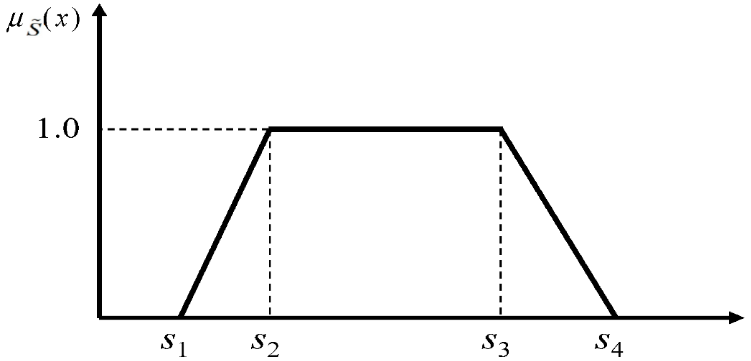
Figure 2.
Framework of extended ORESTE method with TrFNs.
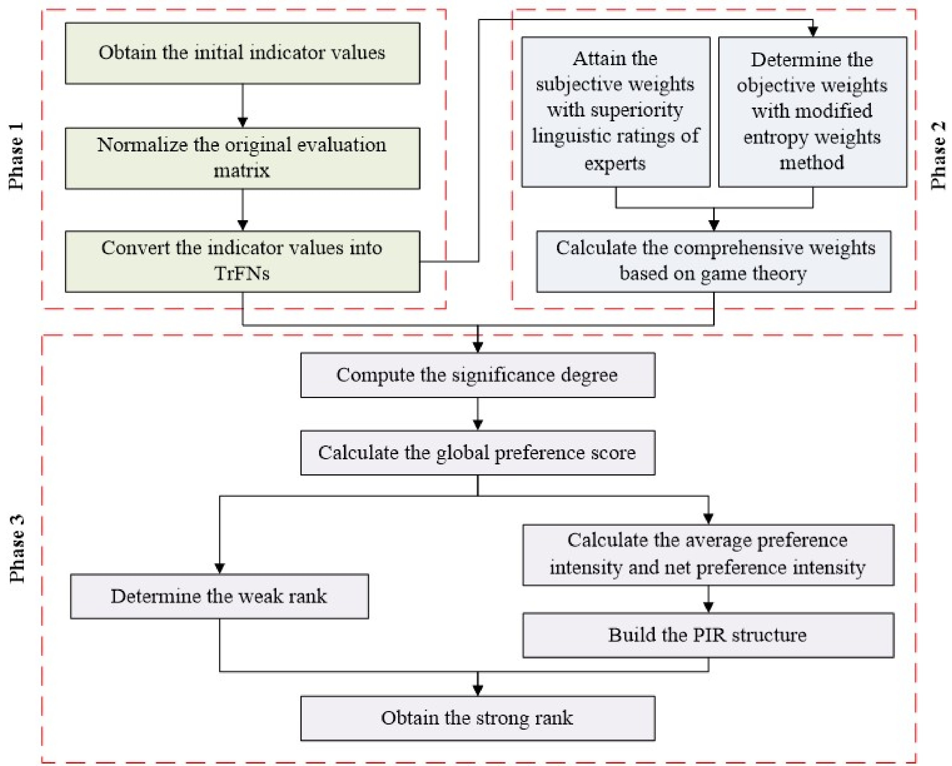
Figure 3.
Location of the Kaiyang phosphate mine.
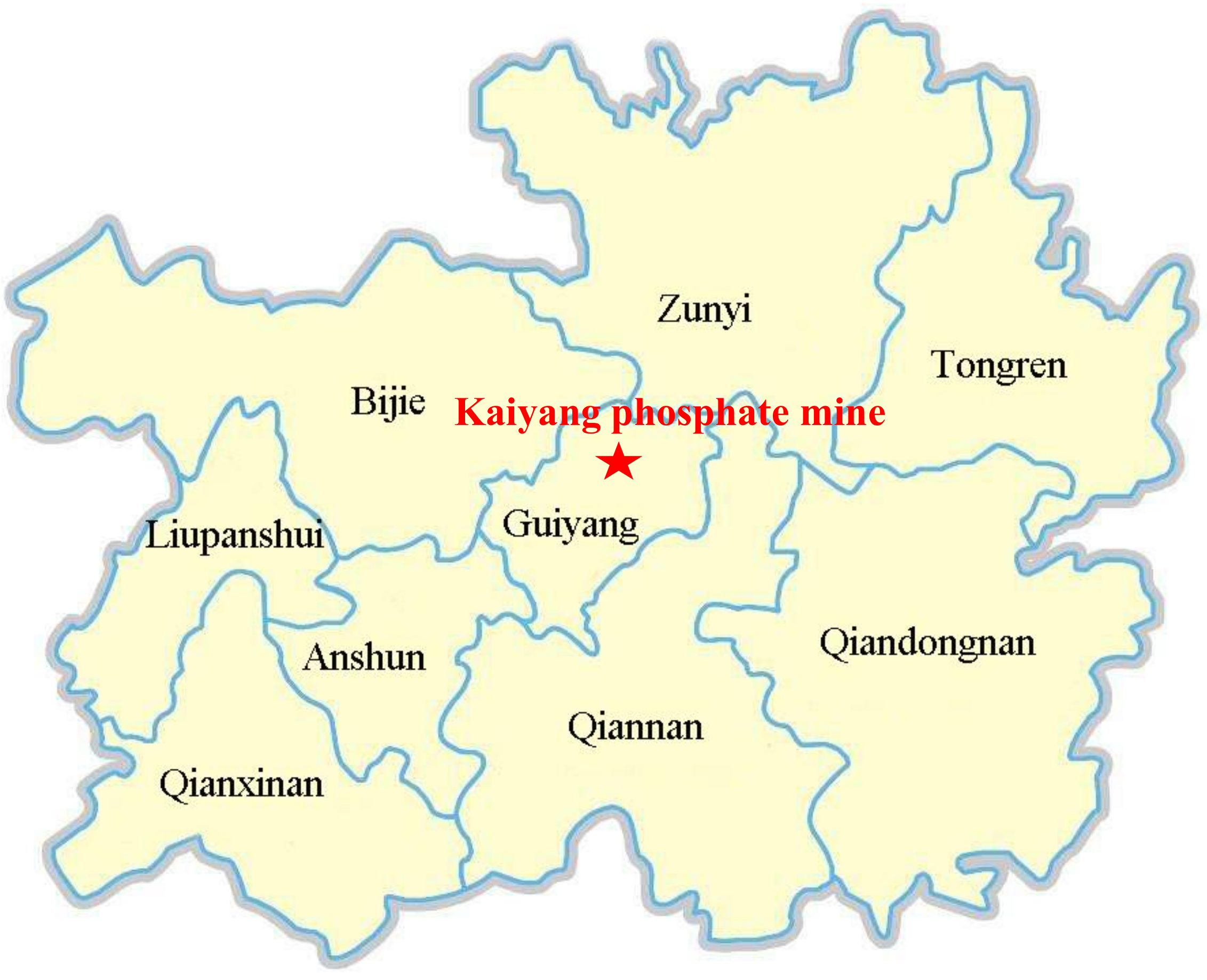
Figure 4.
Values of under different circumstances.
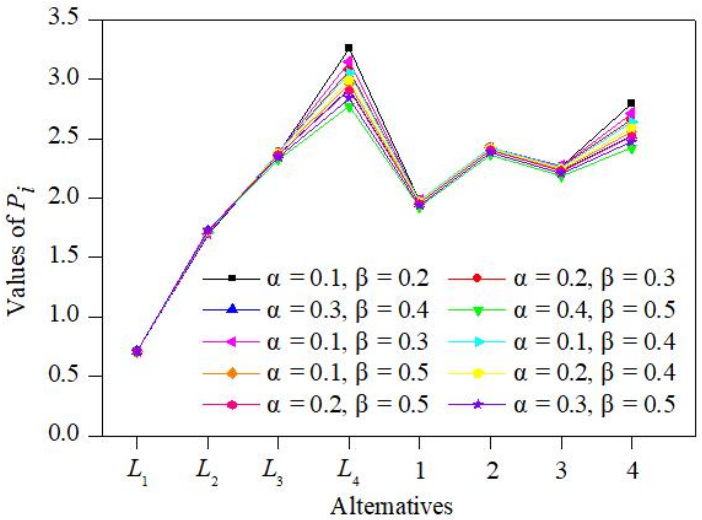
Figure 5.
Values of under different values of and for each indicator.


Table 1.
Interval of indicator values corresponding to each level.
| Indicators | Risk Levels | |||
|---|---|---|---|---|
| >40 | 26.7–40 | 14.5–26.7 | <14.5 | |
| <2.0 | 2.0–3.5 | 3.5–5.0 | >5.0 | |
| <40 | 40–100 | 100–200 | >200 | |
| >14.5 | 5.5–14.5 | 2.5–5.5 | ≤2.5 | |
| <0.50 | 0.50–0.60 | 0.60–0.75 | >0.75 | |
Table 2.
Initial indicator values.
| 40.0 | 0 | 0 | 14.5 | 0 | |
| 26.7 | 2.0 | 40 | 5.5 | 0.50 | |
| 14.5 | 3.5 | 100 | 2.5 | 0.60 | |
| 0 | 5.0 | 200 | 0 | 0.75 | |
| 13.09 | 1.39 | 10.09 | 1.78 | 0.45 | |
| 23.24 | 5.1 | 165.51 | 5.41 | 0.62 | |
| 15.07 | 2.03 | 103.99 | 1.50 | 0.59 | |
| 29.7 | 6.31 | 290.97 | 5.61 | 0.69 |
Table 3.
Normalized decision-making matrix.
| 0.000 | 0.000 | 0.000 | 0.000 | 0.000 | |
| 0.333 | 0.317 | 0.137 | 0.621 | 0.667 | |
| 0.638 | 0.555 | 0.344 | 0.828 | 0.800 | |
| 1.000 | 0.792 | 0.687 | 1.000 | 1.000 | |
| 0.673 | 0.220 | 0.035 | 0.877 | 0.600 | |
| 0.419 | 0.808 | 0.569 | 0.627 | 0.827 | |
| 0.623 | 0.322 | 0.357 | 0.897 | 0.787 | |
| 0.258 | 1.000 | 1.000 | 0.613 | 0.920 |
Table 4.
Fuzzy decision-making matrix.
| (0.00, 0.00, 0.00, 0.00) | (0.00, 0.00, 0.00, 0.00) | (0.00, 0.00, 0.00, 0.00) | (0.00, 0.00, 0.00, 0.00) | (0.00, 0.00, 0.00, 0.00) | |
| (0.27, 0.30, 0.37, 0.40) | (0.25, 0.29, 0.35, 0.38) | (0.11, 0.12, 0.15, 0.17) | (0.50, 0.56, 0.68, 0.74) | (0.53, 0.60, 0.73, 0.80) | |
| (0.51, 0.57, 0.70, 0.77) | (0.44, 0.50, 0.61, 0.67) | (0.27, 0.31, 0.38, 0.41) | (0.66, 0.74, 0.91, 0.99) | (0.64, 0.72, 0.88, 0.96) | |
| (0.80, 0.90, 1.10, 1.200) | (0.63, 0.71, 0.87, 0.95) | (0.55, 0.62, 0.76, 0.82) | (0.80, 0.90, 1.10, 1.20) | (0.80, 0.90, 1.10, 1.20) | |
| (0.54, 0.61, 0.74, 0.81) | (0.18, 0.20, 0.24, 0.26) | (0.028, 0.031, 0.038, 0.042) | (0.70, 0.79, 0.97, 1.05) | (0.48, 0.54, 0.66, 0.72) | |
| (0.34, 0.38, 0.46, 0.50) | (0.65, 0.73, 0.89, 0.97) | (0.46, 0.51, 0.63, 0.68) | (0.50, 0.56, 0.69, 0.75) | (0.66, 0.74, 0.91, 0.99) | |
| (0.50, 0.56, 0.69, 0.75) | (0.26, 0.29, 0.35, 0.39) | (0.29, 0.32, 0.39, 0.43) | (0.72, 0.81, 0.99, 1.08) | (0.63, 0.71, 0.87, 0.94) | |
| (0.21, 0.23, 0.28, 0.31) | (0.80, 0.90, 1.10, 1.20) | (0.80, 0.90, 1.10, 1.20) | (0.49, 0.55, 0.67, 0.74) | (0.74, 0.83, 1.01, 1.10) |
Table 5.
Linguistic ratings and weights of indicators.
| Indicators | Linguistic Ratings of Indicators | ||||||
|---|---|---|---|---|---|---|---|
| VH | H | M | FH | H | (3.1, 3.6, 3.8, 4.2) | 0.1883 | |
| H | VH | VH | H | FH | (3.5, 4.0, 4.3, 4.6) | 0.2099 | |
| H | VH | H | FH | H | (3.4, 3.9, 4.1, 4.5) | 0.2037 | |
| FH | FH | VH | VH | H | (3.3, 3.8, 4.2, 4.5) | 0.2023 | |
| H | M | H | H | VH | (3.3, 3.8, 3.9, 4.3) | 0.1959 | |
Note: VH indicates very high; H indicates high; FH indicates fairly high; and M indicates medium.
Table 6.
Significance degree.
| 0.000 | 0.000 | 0.000 | 0.000 | 0.000 | |
| 0.333 | 0.317 | 0.137 | 0.621 | 0.667 | |
| 0.638 | 0.555 | 0.344 | 0.828 | 0.800 | |
| 1.000 | 0.792 | 0.687 | 1.000 | 1.000 | |
| 0.673 | 0.220 | 0.035 | 0.877 | 0.600 | |
| 0.419 | 0.808 | 0.569 | 0.627 | 0.827 | |
| 0.623 | 0.322 | 0.357 | 0.897 | 0.787 | |
| 0.258 | 1.000 | 1.000 | 0.613 | 0.920 |
Table 7.
Global preference score.
| 0.130 | 0.163 | 0.188 | 0.114 | 0.112 | |
| 0.269 | 0.277 | 0.212 | 0.454 | 0.484 | |
| 0.469 | 0.425 | 0.307 | 0.596 | 0.577 | |
| 0.719 | 0.583 | 0.521 | 0.716 | 0.716 | |
| 0.493 | 0.225 | 0.190 | 0.631 | 0.439 | |
| 0.324 | 0.594 | 0.444 | 0.458 | 0.595 | |
| 0.460 | 0.280 | 0.315 | 0.644 | 0.567 | |
| 0.224 | 0.726 | 0.732 | 0.448 | 0.660 |
Table 8.
Average preference intensity.
| 0.000 | 0.000 | 0.000 | 0.000 | 0.000 | 0.000 | 0.000 | 0.000 | |
| 0.198 | 0.000 | 0.000 | 0.000 | 0.024 | 0.000 | 0.000 | 0.010 | |
| 0.333 | 0.136 | 0.000 | 0.000 | 0.091 | 0.057 | 0.033 | 0.079 | |
| 0.510 | 0.312 | 0.176 | 0.000 | 0.256 | 0.170 | 0.198 | 0.164 | |
| 0.254 | 0.080 | 0.012 | 0.000 | 0.000 | 0.069 | 0.007 | 0.090 | |
| 0.342 | 0.144 | 0.065 | 0.002 | 0.156 | 0.000 | 0.094 | 0.022 | |
| 0.312 | 0.114 | 0.011 | 0.000 | 0.064 | 0.064 | 0.000 | 0.086 | |
| 0.417 | 0.229 | 0.162 | 0.071 | 0.253 | 0.097 | 0.191 | 0.000 |
Table 9.
Net preference intensity.
| 0.000 | −0.198 | −0.333 | −0.510 | −0.254 | −0.342 | −0.312 | −0.417 | |
| 0.198 | 0.000 | −0.136 | −0.312 | −0.056 | −0.144 | −0.114 | −0.219 | |
| 0.333 | 0.136 | 0.000 | −0.176 | 0.079 | −0.008 | 0.022 | −0.083 | |
| 0.510 | 0.312 | 0.176 | 0.000 | 0.256 | 0.168 | 0.198 | 0.093 | |
| 0.254 | 0.056 | −0.079 | −0.256 | 0.000 | −0.087 | −0.058 | −0.162 | |
| 0.342 | 0.144 | 0.008 | −0.168 | 0.087 | 0.000 | 0.030 | −0.075 | |
| 0.312 | 0.114 | −0.022 | −0.198 | 0.058 | −0.030 | 0.000 | −0.105 | |
| 0.417 | 0.219 | 0.083 | −0.093 | 0.162 | 0.075 | 0.105 | 0.000 |
Table 10.
PIR structure of alternatives.
| - | O | O | O | O | O | O | O | |
| P | - | O | O | I | O | O | O | |
| P | P | - | O | I | I | I | O | |
| P | P | P | - | P | P | P | P | |
| P | I | I | O | - | O | I | O | |
| P | P | I | O | P | - | I | I | |
| P | P | I | O | I | I | - | O | |
| P | P | P | O | P | I | P | - |
Table 11.
Evaluation results of empirical methods.
| Authors | Indicators | Evaluation Criteria | Evaluation Results | |||
|---|---|---|---|---|---|---|
| Peng et al. [49] | The intervals of , , and are , , and , respectively. | |||||
| Kidybiński [13] | The intervals of , , and are , , and , respectively. | |||||
| Kwasniewski et al. [50] | The intervals of , , and are , , and , respectively. | |||||
| Tao [15] | The intervals of , , and are , , and , respectively. | |||||
| Wang et al. [28] | The intervals of , , and are , , and , respectively. | |||||
Table 12.
Evaluation results of other MCDM methods.
| Authors | Evaluation Methods | Evaluation Results |
|---|---|---|
| Mahdavi et al. [44] | Trapezoidal fuzzy TOPSIS method | |
| Wang and Li [51] | Trapezoidal fuzzy TODIM method | |
| The proposed method | Trapezoidal fuzzy ORESTE method | Weak rank: |
| Strong rank: |
Table 13.
Evaluation results under different and values.
| Value of | Value of | Evaluation Results |
|---|---|---|
| 0.1 | 0.2 | Weak rank: |
| Strong rank: | ||
| 0.2 | 0.3 | Weak rank: |
| Strong rank: | ||
| 0.3 | 0.4 | Weak rank: |
| Strong rank: | ||
| 0.4 | 0.5 | Weak rank: |
| Strong rank: | ||
| 0.1 | 0.3 | Weak rank: |
| Strong rank: | ||
| 0.1 | 0.4 | Weak rank: |
| Strong rank: | ||
| 0.1 | 0.5 | Weak rank: |
| Strong rank: | ||
| 0.2 | 0.4 | Weak rank: |
| Strong rank: | ||
| 0.2 | 0.5 | Weak rank: |
| Strong rank: | ||
| 0.3 | 0.5 | Weak rank: |
| Strong rank: |
Table 14.
Evaluation results under different values of and for each indicator.
| Number | Value of | Value of | Evaluation Results | ||||||||
|---|---|---|---|---|---|---|---|---|---|---|---|
| 0.1 | 0.2 | 0.3 | 0.4 | 0.5 | 0.2 | 0.3 | 0.4 | 0.5 | 0.6 | Weak rank: | |
| Strong rank: | |||||||||||
| 0.5 | 0.4 | 0.3 | 0.2 | 0.1 | 0.6 | 0.5 | 0.4 | 0.3 | 0.2 | Weak rank: | |
| Strong rank: | |||||||||||
| 0.2 | 0.3 | 0.4 | 0.5 | 0.6 | 0.3 | 0.4 | 0.5 | 0.6 | 0.7 | Weak rank: | |
| Strong rank: | |||||||||||
| 0.6 | 0.5 | 0.4 | 0.3 | 0.2 | 0.7 | 0.6 | 0.5 | 0.4 | 0.3 | Weak rank: | |
| Strong rank: | |||||||||||
| 0.3 | 0.4 | 0.5 | 0.6 | 0.7 | 0.4 | 0.5 | 0.6 | 0.7 | 0.8 | Weak rank: | |
| Strong rank: | |||||||||||
| 0.7 | 0.6 | 0.5 | 0.4 | 0.3 | 0.8 | 0.7 | 0.6 | 0.5 | 0.4 | Weak rank: | |
| Strong rank: | |||||||||||
| 0.4 | 0.5 | 0.6 | 0.7 | 0.8 | 0.5 | 0.6 | 0.7 | 0.8 | 0.9 | Weak rank: | |
| Strong rank: | |||||||||||
| 0.8 | 0.7 | 0.6 | 0.5 | 0.4 | 0.9 | 0.8 | 0.7 | 0.6 | 0.5 | Weak rank: | |
| Strong rank: | |||||||||||
Publisher’s Note: MDPI stays neutral with regard to jurisdictional claims in published maps and institutional affiliations. |
© 2022 by the authors. Licensee MDPI, Basel, Switzerland. This article is an open access article distributed under the terms and conditions of the Creative Commons Attribution (CC BY) license (https://creativecommons.org/licenses/by/4.0/).
Share and Cite
MDPI and ACS Style
Shi, K.; Liu, Y.; Liang, W. An Extended ORESTE Approach for Evaluating Rockburst Risk under Uncertain Environments. Mathematics 2022, 10, 1699. https://doi.org/10.3390/math10101699
AMA Style
Shi K, Liu Y, Liang W. An Extended ORESTE Approach for Evaluating Rockburst Risk under Uncertain Environments. Mathematics. 2022; 10(10):1699. https://doi.org/10.3390/math10101699
Chicago/Turabian StyleShi, Keyou, Yong Liu, and Weizhang Liang. 2022. "An Extended ORESTE Approach for Evaluating Rockburst Risk under Uncertain Environments" Mathematics 10, no. 10: 1699. https://doi.org/10.3390/math10101699
Note that from the first issue of 2016, this journal uses article numbers instead of page numbers. See further details here.